比較西歐銀行業之成本效率：新共同邊界Fourier成本函數之應用 - 政大學術集成

全文

(1)國立政治大學商學院金融學系博士論文 Department of Money and Banking College of Commerce. National Chengchi University Doctoral Dissertation. 比較西歐銀行業之成本效率：治. 政. 大. 立 Fourier 成本函數之應用新共同邊界. ‧ 國. 學. Comparing Cost Efficiency in Western European. ‧. Banking Industries: Using the New Metafrontier. n. al. er. io. sit. y. Nat. Fourier Flexible Cost Function. Ch. engchi. i Un. v. 指導教授：黃台心博士研究生：李起銓撰. 中華民國一○二年七月 July, 2013.

(2) 誌謝隨著論文的完成，博士班的求學生涯即將劃下句點，學習過程中的甘甜苦澀，一幕幕的在腦海中來回播放，心中除了些許的感慨，更多的是無限的喜悅、感動以及感恩，要感謝的人實在太多了，無法一一道盡，但你們的支持與鼓勵永遠是我前進的最大動力。本論文得以順利完成，首要感謝指導教授. 黃台心老師的悉心指導，承蒙恩. 師在學識的養成及研究上的啟蒙與教導，奠定了研究論文之基礎，恩師對於研究的專注與熱忱，更是學生努力學習的方向與目標，學生由衷地的感謝老師的諄諄教誨，無論在學習及待人處事，都讓學生獲益良多，能在老師的指導下學習是學. 治政生的榮幸，老師及師母對於學生的關心與鼓勵，學生銘感於心。同時，也要感謝大立口試委員王泓仁老師、胡均立老師、陳坤銘老師、林建秀老師細心審閱學生的論 ‧ 國. 學. 文，在口試期間提供諸多寶貴意見，給予學生許多啟發，使得本論文內容更臻充. ‧. 實與完備。此外，也要感謝沈中華老師對學生的指導與照顧，李建強老師、許義. sit. y. Nat. 忠老師、楊淑玲老師、陳獻儀老師，在學生求學生涯裡，一路的陪伴與一直的支. io. er. 持與鼓勵，總是在學生徬徨無助時，指引學生方向，在此謹致最誠摰的感謝。在博士班就讀期間，感謝系上老師扎實的學科訓練，感謝立璿、怡慧、子雄、. al. n. iv n C 惠龍哥、銘泰、嘉晃、育民等同窗好友在求學的過程中相互陪伴、勉勵與學習， hengchi U. 感謝秉倫學長、冠臻學姐、淑華學姐對我在課業上的幫助以及不時的加油打氣，感謝淑芳助教，明潔助教在行政事務上總是提供最高品質的幫忙與協助。此外，銀五乙的摯友們、龍騰伙伴們，以及讀書會的成員們，無論在過去或是未來，為我的生活增添許多色彩，是我生命中最珍貴的寶藏。最後，要特別感謝我的父母及家人，每每在我覺得疲累時，給予我最大的關懷與鼓勵，全心全意的付出與支持，使我能夠無後顧之憂的全力追求夢想，感謝您的養育之恩、栽培之情，心中的無限感激筆墨難以形容，也要感謝摯愛的太太惠瑜，一路的相伴與扶持，細心照顧我的生活起居，感謝生命中有妳。.

(3) 僅以本論文獻給我的家人及關愛我的師長及友人. 李起銓. 謹致於. 國立政治大學金融學系中華民國一○二年七月. 立. 政治大. ‧. ‧ 國. 學. n. er. io. sit. y. Nat. al. Ch. engchi. 3. i Un. v.

(4) 摘要本文採用新的隨機共同邊界方法，將其擴充至 Fourier 富伸縮成本函數，針對西歐地區十個國家的銀行業進行成本效率之分析，資料期間涵蓋 1996 年至 2010 年。不同於 Battese et al. (2004), O’Donnell et al. (2008), and Huang et al. (2011a) 等人利用線性規劃法，本文應用隨機共同邊界法來估計技術缺口比率，進而做跨國間的效率比較，此法的特點在於技術缺口比率可以設為一些反映國家環境差異的外生變數之函數，而線性規劃法則無法做此設定。實證結果顯示採用線性規劃方法所估計出的技術缺口比率與共同成本效率會有低估的現象，技術缺口比率以及共同成本效率在 1996 年至 2000 年間逐步上升，此結果支持金融市場的整合可以. 治政增進效率，然而，到 2000 年之後則反轉向下，特別是在大 2007 年至 2010 年次級立房貸風暴時期明顯惡化。此外，進一步的分群進行分析的結果顯示，小規模、高 ‧ 國. 學. 獲利、或是較保守的銀行相對來說較具有效率。. ‧ sit. y. Nat. io. er. 關鍵詞：共同邊界、成本效率、技術缺口比率、環境變數 JEL 分類代號：C51 • G21 • D24. n. al. Ch. engchi. i Un. v.

(5) Abstract This paper aims to gain further insights into cost efficiency using the newly developed metafrontier approach under the framework of the Fourier flexible cost frontier for banking industries across 10 Western European nations during the period 1996-2010. Unlike Battese et al. (2004), O’Donnell et al. (2008), and Huang et al. (2011a), who suggest using programming techniques, the stochastic metafrontier is formulated and applied to obtain the technology gap ratio (TGR) for efficiency comparisons among countries. One salient feature of our method is that the TGR can be specified as a function of some exogenous variables that reflect group-specific environmental. 治政 differences, while the mathematical programming is not 大allowed to do so. Empirical 立 results show that both TGR and metafrontier cost efficiency (MCE) are ‧ 國. 學. underestimated by programming techniques. The TGR and MCE exhibit a gradual. ‧. upward trend during 1996-2000 and then followed by a downward trend, especially. sit. y. Nat. after the subprime crisis of 2007-2010. This suggests that a more integrated financial. io. er. market is able to improve banking efficiency. Smaller banks tend to be more cost efficient than larger ones. Higher profitable banks and more conservative banks are. n. al. related to greater efficiency.. Ch. engchi. i Un. v. Keywords: Metafrontier; Cost efficiency; Technology gap ratio; Environmental variables; JEL classification: C51 • G21 • D24.

(6) Contents. 1. Introduction. 1. 2. An Overview of Recent Literature. 6. 2.1 The Metafrontier Model ……………………………………………………6 2.2 Western European Banking Performance …………………………………..7 3. Methodology. 13. 3.1 The Fourier Flexible Cost Function ………………………………………..13 3.2 Metafrontier FF Cost Function and Technology Gaps ……………………..14. 學. ‧ 國. 4.. 治政 3.3 Estimation Procedure ………………………………………………………17 大立 Data Description 20. 5. Empirical Results and Analysis. 32. ‧. 5.1 Parameter Estimates ………………………………………………………..32. sit. y. Nat. 5.2 Cost Efficiencies and Technology Gaps ……………………………………41. io. er. 5.3 Global Views on the Trend …………………………………………………50 5.4 Relationships between Efficiencies and Bank Characteristics ……………..56. n. al. 6. Conclusion Appendix A. Ch. engchi. i Un. v. 64 77. Appendix B. 88. Appendix C. 93. Appendix D. 99.

(7) List of Tables. Table 1. Listing of selected studies of West European banking Efficiency by distinct frontier techniques ……………………………………………………… ..9. Table 2. Summary of variables, descriptions, and data sources …………………. 22. Table 3. Summary statistics for banking costs, outputs, inputs, and input prices .. 23. Table 4. Listing of selected environmental variables used as determinants of efficiency in recent studies ……………………………………………... 24. Table 5. Summary statistics for environmental variables ………………………... 30. Table 7. Parameter estimates of the environmental variables ……………………. 35. Table 8. Summary statistics for CE measures by different cost function setting …37. Table 9. Parameter estimates for various competing metafrontier models (FF) …. 39. Table 10. Summary statistics of relevant efficiency scores for various competing. ‧. ‧ 國. 學. Table 6. 治政 Parameter estimates of the Fourier flexible 大 cost frontier for the sample 立 countries ………………………………………………………………… 33. er. io. sit. y. Nat. metafrontier models based on FF specification ……………………….. 42. al. n. iv n C Summary statistics of relevant scores for various competing h e nefficiency gchi U. Table 11. metafrontier models based on TL specification ……………………….. 48. Table 12. Summary statistics of relevant efficiency scores over time (SMF95-FF) .51. Table 13. Summary statistics of relevant efficiency scores over time (SMF95-TL) .55. Table 14. Summary statistics of relevant efficiency scores by asset sizes, return on assets and the ratio of equity to total assets (SMF95) ………………….. 57. Table 15. Summary statistics of relevant efficiency scores by asset sizes, return on assets and the ratio of equity to total assets (SMF95) …………………...61.

(8) List of Figures. Figure 1 Metafrontier cost model …………………………………………………17 Figure 2 Mean values of CE by country (FF versus TL) …………………………. 37 Figure 3. Scatter diagram of CE and TGR in mean ……………………………….. 45. Figure 4 Mean values of TGR and MCE by country for various competing models …………………………………………………………………...47 Figure 5 Trends in CE, TGR, and MCE (SMF95-FF) …………………………... 52 Figure 6 Trends in CE, TGR, and MCE (SMF95-TL) …………………………... 56 Figure 7. 58 58. 學. ‧ 國. Figure 8. 治政 Trends in CE, TGR, and MCE by size class大 (SMF95-FF) …………….. 立 Trends in CE, TGR, and MCE by ROA class (SMF95-FF) ……………. Figure 9 Trends in CE, TGR, and MCE by ETA class (SMF95-FF) ……………. 59. ‧. Figure 10 Trends in CE, TGR, and MCE by size class (SMF95-TL) …………... 62. sit. y. Nat. Figure 11 Trends in CE, TGR, and MCE by ROA class (SMF95-TL) …………… 62. io. n. al. er. Figure 12 Trends in CE, TGR, and MCE by ETA class (SMF95-TL) …………. 63. Ch. engchi. i Un. v.

(9) 1. Introduction The financial services industries in Western European countries have become highly integrated ever since the completion of the Single Market for Financial Services in 1993. Banking industries there have experienced a wide range of fundamental changes in their regulatory and competitive environments, including the reduction or elimination of trade and entry barriers to those markets in the European Union (EU). Banks are soon facing an increasingly competitive atmosphere not only from domestic markets, but also from abroad. Bank managers must adopt the best technologies to efficiently produce an array of financial products in order to gain. 治政 excess profit and to be viable. In this wave of international 大 economic integration, the 立 cost efficiency of EU banks is a core issue worth to be deeply investigated. ‧ 國. 學. Banks tend to take up more risk as the global economy becomes increasingly. ‧. integrated and liberalized. As noted by González (2005) and Fiordelisi et al. (2011),. sit. y. Nat. the growing competition reduces the market power of banks thereby reducing their. io. er. charter value. Chortareas et al. (2013) point out that excessive financial liberalization might provide an incentive for financial institutions to take greater risks, which might. n. al. incur recent subprime crisis. iv n C and hEuropean crises. U e n g c h i In addition,. banks in such an. integrated and interconnected market as the EU are more likely to be exposed to global shocks (Camilla et al., 2013). How to successfully weather the financial crisis, particularly in the future, appears to be an important topic, and this is intimately associated with banks’ efficiency, since a cost efficient bank is able to offer various financial services to its customers in a lower cost and earn higher profits. This prompts the initial motivation for this study, aiming at investigating the efficiency of Western European banking industries. Many previous studies that carry out international comparisons among banks of different nations estimate either a common frontier for those banks by pooling all 1.

(10) observations together, or a group (country) specific frontier for each nation. The former approach implicitly assumes that banks from different countries have access to the same technology, which appears to be impractical, since each country has its own cultural traditions, resource endowments, and political and legal systems. These characteristics affect the behavior and willingness of banks to undertake new innovations. Different regulatory environments, for example, lead to either universal banking countries, such as Germany and Switzerland, or separated banking countries such as Belgium and the US (Allen and Rai, 1996). Universal banking countries permit commercial banks to engage in nontraditional activities such as investment,. 治政 trading, real estate, and insurance, while separated banking 大 countries do not. Barth et 立 al. (2004) and Chortareas et al. (2012) describe some of the background information ‧ 國. 學. on regulatory and supervisory differences.. ‧. The latter approach attempts to obtain individual production frontiers for each. sit. y. Nat. country, which allows for measuring the country-specific efficiency scores for each. io. er. sample bank. This method avoids making the strong assumption that all banks of different countries under consideration share the same technology. However, the. al. n. iv n C so-derived efficiency scores are nothcomparable due to e n g c h i Uthe fact that they are evaluated. against different frontiers that represent dissimilar standard. The foregoing dilemma motivates Battese et al. (2004) and O’Donnell et al. (2008) to propose a mixed two-step approach to find the metafrontier production function that facilitates efficiency comparisons of different groups. Their two-step procedure combines the conventional stochastic frontier approach (SFA) in the first step to estimate the group-specific frontiers with the mathematical programing technique in the second step to estimate the mefafrontier production function. Clearly, these two steps involve the use of distinct approaches, i.e., the econometric and non-parametric approaches. The former requires specifying a 2.

(11) specific functional form with statistical noise, while the latter is function-free and unable to immune from random shocks. One potential limitation on the programming technique is that the parameter estimates are lack of statistical properties due to the linear (or quadratic) programming is deterministic in essence and its estimates are inclined to be confounded with shocks. Although Battese et al. (2004) suggest using simulation and bootstrapping methods to derive standard errors of the coefficient estimates, no statistical properties of the coefficient estimates and their standard errors have been inferred. Furthermore, to adjust for the effects of environments on the efficiency of a bank, the programming technique has to rely on, e.g., the two-stage. 治政 method or three-stage methods (Fried et al. 2002). Conversely, the SFA of Battese 大立 and Coelli (1995) enables ones to examine the determinants of the efficiency scores in 1. ‧ 國. 學. a single step.2. ‧. The current paper employs the newly developed model by Huang et al. (2012) to. sit. y. Nat. estimate and compare the cost efficiencies of banks in Western European countries.. io. er. The major difference between the new approach and the mixed approach of Battese et al. (2004) and O’Donnell et al. (2008) lies in the second step relating to the estimation. al. n. iv n C of the metafrontier. Specifically, the U second step of the new model hmetafrontier e n g c hini the is still estimated by the SFA, rather than the linear or quadratic programming (QP). In. this manner, the parameter estimates and their standard errors have known statistical properties. In addition, the technology gap ratio can be specified as a set of environmental variables, characterizing the exogenous differences faced by groups or countries. We can also refer the new metafrontier as the stochastic metafrontier (SMF), as opposed to the deterministic metafrontier derived by the mixed approach. 1. The method involves solving a linear programming problem to obtain some efficiency measures in a first-stage analysis. In the second stage, one regresses the measures from the first stage upon the environmental variables. 2 Wang and Schmidt (2002) find evidence supporting one-step models whenever one is interested in the effects of exogenous variables on efficiency levels, in which their analysis is based on the “scaling property”. 3.

(12) In summary, the present study attempts to extend the deterministic metafrontier translog (TL) cost function to the more general SMF Fourier flexible (FF) cost function that has several advantages. First, since the technology parameters of the SMF are estimated by the maximum likelihood (ML), the conventional statistical inferences for parameter estimates can be directly drawn without relying on simulations or bootstrapping techniques. Second, the technology gaps can be treated as a one-sided error term, which, together with the statistical noise, constitutes the composed error. Finally, macroeconomic environmental conditions can be modeled as the determinants of the technology gaps, like the one proposed by Battese and Coelli. 治政 (1995). The variance of the one-sided error term is heteroscedastic, as pointed out by 大立 Kumbhakar and Lovell (2003), which may be preferable and consistent with reality. ‧ 國. 學. Although the translog cost function has been widely used by numerous. ‧. practitioners to characterize the production technology of banking sectors, it is. sit. y. Nat. criticized as being merely able to locally approximate a true but unknown cost. io. er. function, forcing large and small banks to lie on a symmetric U-shaped ray average cost curve, and producing biased measures of scale economies for bans of various. al. n. iv n C sizes. See, for example, McAllister (1993), Wheelock and Wilson h eandn gMcManus chi U (2001), and Huang and Wang (2004). In contrast, the FF functional form of Gallant. (1982) is the global approximation to the underlying cost function as closely as desired in Sobolev norm. Many empirical studies confirm that the FF function provides a better fit for financial institution data than the translog specification, e.g., McAllister and McManus (1993), Mitchell and Onvural (1996), Berger and Mester (1997), and Berger et al. (1997). The FF has now received more emphasis in the recent efficiency literature, e.g., Altunbaş et al. (2000, 2001a, b), Williams and Gardener (2003), Kraft et al. (2006), Das and Das (2007), Beccalli and Frantz (2009), Feng and Serletis (2009), Huang et al. (2011a, b), to mention a few. Therefore, the FF 4.

(13) cost function should be a preferable choice to the standard translog form and can better describe the underlying technology adopted by banking sectors. On the basis of the above framework, this paper is capable of assessing and comparing the efficiency scores among the banking industries of EU members under the uniform benchmark, i.e., the estimated metafrontier FF cost function. More specific, the bank-specific environmental variables are taken into account in the first step when the individual country-specific FF cost frontiers are estimated for each country. Next, the macroeconomic environmental variables are considered in the second step when the metafrontier FF cost function is estimated. These efforts intend. 治政 to further shed light on banks’ performance in Western大 European countries during the 立 transition period of financial reform, market integration, and financial crisis. ‧ 國. 學. The rest of the paper is organized as follows. Section 2 briefly reviews the. ‧. literature on metafrontier model and empirical studies specifically about banks’. sit. y. Nat. efficiency in Western European countries. Section 3 formulates the metafrontier FF. io. er. cost function and depict the estimation procedure. Section 4 introduces the data and variable definitions. Section 5 conducts the empirical study, while the last section. n. al. concludes the paper.. Ch. engchi. 5. i Un. v.

(14) 2. An Overview of Recent Literature This section first describes the development of matafrontier models, and then reviews the relevant empirical researches, particularly focusing on cross-country comparisons of banking efficiency in Western European countries, as well as some measurement problems.. 2.1 The Metafrontier Model The idea of metaproduction function is first proposed by Hayami (1969) and Hayami and Ruttan (1970, 1971). Later, Lau and Yotopoulos (1989) address some. 治政 econometric advantages of applying the metaproduction 大 function. Recently, Battese 立 and Rao (2002) develop the SMF model that pools the data of all groups in ‧ 國. 學. formulating the metafrontier. Their model has often been criticized as being. ‧. inconsistent in the data generating process (DGP), because they assume two different. sit. y. Nat. data-generation mechanisms pertaining to the group and the matafrontier.. io. er. Battese et al. (2004) soon revise the foregoing model by specifying a single data-generation process for firms of different groups. They have potential access to. al. n. iv n C the same technology, but each group choose to operate on different part of the h emay ngchi U. production possibility curve, depending on resource endowments, relative input prices, adoption of technology, and specific circumstances of economic and political systems. In this context, a metafrontier function is an overarching function that encompasses the deterministic components of the group specific production frontiers. O’Donnell et al. (2008) subsequently utilize both DEA (data envelopment analysis) and SFA techniques to estimate the technical efficiencies against the group frontiers and. technology gaps between the group frontiers and the metafrontier. Huang et al. (2011a) further extend the primal production frontier setting to the dual cost frontier specification. The primary advantage of the cost frontier lies in its ability to consider 6.

(15) the case of multiple outputs and inputs, making it particularly suitable for characterizing multi-output firms such as financial institutions and insurance companies. Although the metafrontier approach allows researchers to correctly perform efficiency comparison among different groups and has drawn much attention to academic researchers, e.g., Bos and Schmiedel (2007), Chen and Song (2008), Moreira and Bravo-Ureta (2010), Mariano et al. (2011), and Lu and Chen (2012), it suffers from some potential methodological limitations as mentioned in the previous section. A more recent study by Huang et al. (2012) elaborate the metafrontier. 治政 production function and propose a new two-step approach 大 to construct the SMF. This 立 novel approach first estimates technical efficiency with respect to group-specific ‧ 國. 學. frontiers, followed by measuring the technology gap ratio with respect to the. ‧. metafrontier under the framework of the SFA, instead of using mathematical. sit. y. Nat. programming techniques. It can be shown that the model of Battese et al. (2004) and. io. er. O’Donnell et al. (2008) is a special case of the new two-step approach.. n. al. 2.2. i n Western European BankingC Performance U hengchi. v. Recently, the efficiency measurement of banking industries is of great concern because of the prevalence of deregulation, globalization, and financial innovation in the industry, as well as the intensified competition that raises operation and global risks. In the ongoing integration of European financial markets, the structure of banking industries has experienced rapid changes. Whether the efficiency scores of European banks tends to be equalized is an interesting issue and worth thoroughly investigated. Different frontier approaches based on either parametric or nonparametric techniques have been carried out in order to evaluate and compare banks’ efficiencies in Western Europe and other areas. Berger and Humphrey (1997), 7.

(16) Goddard et al. (2001), Berger (2007), Fethi and Pasiouras (2010), and Hughes and Mester (2012) offer excellent reviews on this matter. Table 1 summarizes the relevant literature with a particular focus on international comparison of banking efficiencies in Western European countries. Many earlier works have already performed cross-country comparisons by estimating a global cost frontier for the commercial banks in European countries. Allen and Rai (1996) adopt both SFA and DFA (distribution-free approach) to compare cost efficiency (CE) measures across 15 developed countries (including 11 Western European countries) for the period 1988-1992. They divide those sample. 治政 countries into universal banking and separated banking 大 countries, corresponding to 立 different regulatory environments. Using a translog specification, evidence is found ‧ 國. 學. that universal banks are more efficient than those of non-universal banks, and. ‧. financial institutions in France, Italy, United Kingdom, and United State are the most. sit. y. Nat. inefficient. Altunbaş et al. (2001a) extends the translog cost frontier to the FF cost. io. er. frontier and analyze banking efficiency of 15 European countries during the period 1989-1997. Their empirical results suggest that banks can save total costs by reducing. al. n. iv n C inefficiencies. X-inefficiency of h eThe ngchi U. managerial and other. EU banks reveals a. gradually decreasing secular trend over the sample period.. The above studies attempt to construct a common frontier for all banks from different countries, implicitly assuming that banks from various countries undertake a common production technology. Even though this setting allows for a direct comparison of efficiency levels, it fails to account for potential technology heterogeneity among sample countries, leading to misspecification. Meanwhile, the roles played by environmental variables on the determination of a bank’s cost efficiency have drawn much attention to empirical researchers. See, for example, Dietsch and Lozano-Vivas (2000), Cavallo and Roosi (2002), Lozano-Vivas et al. 8.

(17) Table 1 Listing of selected studies of West European banking Efficiency by distinct frontier techniques Countries. Part A. Common frontier Allen and Rai (1996) Austria, Belgium, Denmark, Finland, France, Germany, Italy, Spain, Sweden, Switzerland, UK Altunbaş et al. (2001a) Austria, Belgium, Denmark, Finland, France, Germany, Greece, Ireland, Italy, Luxembourg, Netherlands, Portugal, Spain, Sweden, UK Vennet (2002) Austria, Belgium, Denmark, Finland, France, Germany, Greece, Ireland, Italy, Luxembourg, Netherlands, Norway, Portugal, Spain, Sweden, Switzerland, UK Casu and Girardone France, Germany, Italy, Spain, UK (2004). 1988-1992. SFA, DFA / TL. CE. SFA / FF. CE. SFA / TL, FF. CE, PE. SFA, DEA / FF, TL. CE, PE. DFA / TL. CE. n. Ch. iv 1993 n U. DEA, B&M (1996). TE. engchi. 1993. DEA, B&M (1996). TE. 1992-1997. SFA, B&C (1995) / TL. CE. 1993-1997. DEA, Tobit / n.a.. TE. 9. 1995-1996. 1993-1997. sit. y. ‧. io. Measures. 學. Nat. Part B. Common frontier with environmental variables Dietsch and France, Spain Lozano-Vivas (2000) Lozano-Vivas et al. Belgium, Denmark, France, Germany, Italy, (2001) Luxembourg, Netherlands, Portugal, Spain, UK Lozano-Vivas et al. Belgium, Denmark, France, Germany, Italy, (2002) Luxembourg, Netherlands, Portugal, Spain, UK Cavallo and Roosi France, Germany, Italy, Netherlands, Spain, UK (2002) Casu and Molyneux France, Germany, Italy, Spain, UK. al. Methods / Specifications. 1989-1997 政治大. ‧ 國. 立. Period. 1988-1992. er. Authors.

(18) 1990-1998. SFA, B&C (1995) / FF. CE. Italy, UK 1995-1998 Austria, Belgium, Denmark, Finland, France, Germany, 1991-2005 Greece, Iceland, Ireland, Italy, Luxembourg, Netherlands, Norway, Portugal, Spain, Sweden, Switzerland, UK Austria, Belgium, Denmark, Finland, France, Germany, 2001-2009 Greece, Ireland, Italy, Luxembourg, Netherlands, Portugal, Spain, Sweden, Switzerland, UK. SFA, B&C (1995) / TL SFA, B&C (1995) / FF. CE CE, PE. DEA, truncated regression / n.a.. TE. SFA / FF SFA, DEF, DEA / FF. CE, PE CE. 立. 政治大. 學. ‧ 國. y. Austria, Belgium, Denmark, France, Germany, Greece, Italy, Luxembourg, Netherlands, Norway Portugal, Spain, Sweden, Switzerland, UK Austria, Belgium, France, Germany, Italy, Spain,. io. al. n. Kontolaimou and Tsekouras (2010) Huang et al. (2011a). 1992-1997 1992-1998. Nat. Part D. Metafrontier Bos and Schmiedel (2007). ‧. Part C. National frontier Berger et al. (2000) France, Germany, Italy, UK, US Weill (2004) France, Germany, Italy, Spain, Switzerland. Ch. engchi. Austria, Belgium, Denmark, France, Germany, Italy, Portugal, Spain, Switzerland. sit. Chortareas (2013). Denmark, France, Germany, Italy, Spain, UK. 1993-2004. SFA, quadratic programming. TL. CE, PE. 1997-2004. DEA. n.a.. TE. 1994-2003. SFA, quadratic programming. FF. CE. er. (2003) Williams and Gardener (2003) Beccalli (2004) Beccalli and Frantz (2009). i n U. Notes: B&M (1996) denotes Banker and Morey (1996); B&C (1995) denotes Battese and Coelli (1995).. 10. v.

(19) (2001,2002), Beccalli (2004), Beccalli and Frantz (2009), Battaglia et al. (2010), who carry out international comparisons among countries using common frontiers that take environmental conditions into account. Cavallo and Roosi (2002) employ the model of Battese and Coelli (1995) and define a bank’s size, bank organization types, and bank balance indicators as the environmental variables. Their results suggest that banks in Germany are more efficient than others. Differing from the conventional use of a common frontier, the metafrontier function proposed by Battese et al. (2004) is so constructed as to envelope the group-specific frontiers of a set of countries. Under this framework, Bos and. 治政 Schmiedel (2007) use the translog cost function to 大 estimate comparable efficiency 立 measures for 15 Western European commercial banks during the period 1993-2004. ‧ 國. 學. They intend to address the question that whether a single European banking market. ‧. shares a common benchmark frontier. The results support the existence of a single. sit. y. Nat. European banking market and the average efficiency measures obtained by the pooled. io. er. (common) frontier tend to underestimate in comparison with those obtained by the metafrontiers. Huang et al. (2011a) extend the metafrontier production function to the. al. n. iv n C metafrontier FF cost function with h time-varying technical e n g c h i U inefficiency. They conclude that the mean TGRs are generally increasing over time and that European banks are inclined to adopt more advanced technology during the sample period. Another strand of contemporary literature compares the efficiency of banks across European nations by estimating individual national frontiers. Berger et al. (2000) claim that estimating individual frontiers avoids the comparison problem arising from the environmental differences across nations. They employ the SFA to estimate the cross-border banking efficiency and compare foreign-owned with domestic-owned banks in France, Germany, Spain, the United Kingdom, and the United States, covering 1992-1997. The outcomes show that domestic banks in these 11.

(20) countries outperform foreign banks in terms of cost efficiency, supporting the home field advantage hypothesis. Weill (2004) estimates the cost efficiency of banks in 5 European countries, i.e., France, Germany, Italy, Spain, and Switzerland, using various methods of the SFA, DFA, and DEA for the period 1992-1998. It is crucial to note that the efficiency scores obtained by the foregoing two papers are in fact not directly comparable, because these measures are gauged against different group frontiers, rather than a common frontier or metafrontier. To sum up, all of the aforementioned works that involve cross-country comparisons of efficiency count on either estimating a common frontier or group. 治政 specific production frontiers, but not both. The common 大frontier approach requires the 立 imposition of homogeneous technology adopted by all banks of different countries, ‧ 國. 學. which is inconsistent with the reality and hence results in biased parameter estimates. ‧. and efficiency measures. Moreover, the individual frontiers approach suffers from the. sit. y. Nat. problem of incomparability arising from heterogeneous benchmarks for banks from. io. er. different countries. The current paper attempts to solve those difficulties under the framework of the new metafrontier FF cost function that seems to be advantageous. n. al. over the mixed approach.. Ch. engchi. 12. i Un. v.

(21) 3. Methodology 3.1 The Fourier Flexible Cost Function The FF function is a semi-parametric approach that expands the standard translog functional form by adding a set of trigonometric Fourier series. See, for example, Altunbaş et al. (2001), Huang and Wang (2003, 2004), and Huang et al. (2011a, b). These additional terms consist of various sine and cosine functions that are mutually orthogonal. Gallant (1982) shows that the FF function is capable of approximating the true (but unknown) function as closely as desired in Sobolev norm. Let W = (W1 ,…,WN )′ be an N-vector of input prices and Y = (Y1 ,…, YM )′ be an. 立. 政治大. 學. ‧ 國. M-vector of output quantities. The FF cost frontier ( ln ft ( X it ) ) of bank i at time t , for a given country (group) j, is formulated as: M. N. m =1. n=2. ( X it ) = a0 + ∑ am ln (Ymit ) + ∑ β n ln (Wnit ) + φ1T. ‧. ln ft. j. y. Nat. er. io. sit. N N 1⎡M M ⎤ + ⎢ ∑∑ δ mk ln Ymit ln Ykit + ∑∑ γ nh ln Wnit ln Whit + φ11T 2 ⎥ 2 ⎣ m =1 k =1 n =1 h =1 ⎦. n. al iv n C +∑∑ ρ ln h Y eln W + ∑ n g c h iψ Uln Y T + ∑θ M. N. m =1 n =1. M. mn. mit. nit. m =1. N. m. mit. n =1. n. ln WnitT. M. +∑ ⎡⎣ Am cos ( zmit ) + Bm sin ( zmit ) ⎤⎦ m =1. M. M. + ∑∑ ⎡⎣ Amn cos ( zmit + znit ) + Bij sin ( zmit + znit ) ⎤⎦ + ε m =1 n =1. (1). where X jit includes all relevant variables in the model, ln Ym and ln Wn are the mth (log)output quantities and the nth (log)input prices, respectively, T represents. the time trend. Since the trigonometric function of sine and cosine are defined over 0 13.

(22) and 2π , notation zm is the re-scaled values of ln Ym (m = 1,…, M) such that it spans in the interval [ 0, 2π ] . Notations α , β , φ , δ , γ , ρ , ψ , θ , A , and B signify the technology parameters to be estimated. The scaled log-output quantities are calculated as zm = λm ( ln Ym + ln dm ) , where. λm = 6 ( ln Ymmax + ln d m ) , ln d m = 0.00001 − ln Ymmin , and Ymmax and Ymmin are the maximum and minimum value of output m in the sample. This transformation formula guarantees the minimum value of ln Ym to be slightly greater than zero and. 政治大. the maximum value of ln Ym to be equal to 6 that falls short of 2π . See, Gallant. 立. (1982), Chalfant and Gallant (1985), Mitchell and Onvural (1996), Berger et al.. ‧ 國. 學. (1997), Altunbaş et al. (2000, 2001a, b), Huang and Wang (2004), and Huang et al.. ‧. (2011a, b) to mention a few.. (. ). and. sit. y. Nat. The composed error of ε = v + U contains a two-sided noise v ~ N 0, σ v2. n. al. er. io. a one-sided error U ≥ 0 that reflects cost inefficiency of the firm, where v is. i Un. v. assumed to be independent of U. Following Battese and Coelli (1995), the. Ch. engchi. inefficiency term is associated with an array of environmental variables, that is:. U it = τ it′ Ω + uit ≥ 0 where τ. (2). denotes a collection of environmental variables and Ω is the. (. ). corresponding coefficients, and u ~ N 0, σ u2 .. 3.2 Metafrontier FF Cost Function and Technology Gaps Suppose that there are J different countries and each country has N j banks, facing exogenous input prices and output quantities and attempting to minimize their 14.

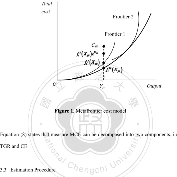
(23) production costs under the constraint of current technology. The stochastic cost frontier model for each bank i ( = 1,… , N j ) of country j ( j = 1,…, J ) at time t ( = 1,…,T ) can be specified as:. C jit = f t j ( X jit ) e. ε jit. (3). Here, C jit is the actual expenditure for bank i of country j at time t , and composed error ε jit = v jit + U jit , where v jit and U jit are similarly defined as the above. The jth country-specific cost frontier of ft j (.) takes the FF form in equation. 政治大. (1), which can vary across country and over time.. 立. The measure of country-specific cost efficiency for bank i of country j at. ‧ 國. 學. v. time t is defined by the ratio of the minimum feasible cost adjusted by noise, e jit , to observed cost, namely:. ‧. v jit. =e. .. (4). sit. C jit. −U jit. y. f t j ( X jit ) e. Nat. CE = j it. er. io. Let ft M ( X jit ) be the underlying metafrontier cost function that envelops all. al. n. iv n C country-specific cost frontiers at time group j’s cost frontier must less than h e tn. Since gchi U. or equal to the metafrontier by definition, their relationship can be expressed as:. f t j ( X jit ) = f t M ( X jit ) e. M U jit. ,. ∀ j , i, t .. (5). Here, term U jitM ≥ 0 measures the gap between country cost frontiers and the metafrontier cost function. Following Battese et al. (2004), the ratio of the metafrontier to the country j’s frontier is defined as the technology gap ratio (TGR), i.e.,. TGR = j it. f t M ( X jit ) f t j ( X jit ). =e. M −U jit. ≤1.. (6) 15.

(24) Here, TGR evaluates the relative deviation of the potential cost defined by the metafrontier FF cost function from the cost of the country frontier FF cost function, holding outputs and input prices constant. This ratio reflects how advance is the production technology adopted by the country, which depends on economic and non-economic environments. Thus, the technology gap component of U jitM can change across firms and countries and over time. The larger the value of the TGR, the more advanced technology the country undertakes, and hence the country frontier is closer to the metafrontier.. 政治大 constructed using the SMF techniques. The stochastic FF cost frontiers for different 立. Figure 1 presents a graphical illustration of how the metafrontier function is. ‧ 國. 學. countries in the case of a single output are denoted by Frontier 1 and Frontier 2 in the figure. The metafrontier cost FF function is drawn as a curve that envelops all. ‧. country-specific cost frontiers. At a given output level Y jit , the difference between a. Nat. io. sit. y. bank’s actual cost C jit and the metafrontier ft M ( X jit ) consists of three components:. er. the technology gap ratio, TGRitj = f t M ( X jit ) ft j ( X jit ) , the bank’s cost efficiency,. n. al. CEitj = f t j ( X jit ) f t j ( X jit ) e. U jit. C jit ft j ( X jit ) e. U jit. =e. v jit. Ch. =e. −U jit. such that. e, nas gwell c hasi. i Un. v. the random noise component,. C jit f t M ( X jit ) = TGRitj × CEitj × e jit . v. We now define the metafrontier cost efficiency (MCE) as the ratio of the metafrontier cost, adjusted for random shocks, to the observed cost:. MCE jit =. f t M ( X jit ) e. v jit. (7). C jit. Substituting equation (3) into equation (7), we obtain. MCE jit =. f t M ( X jit ) ft. j. (X ). e. −U jit. = TGRitj × CEitj .. jit. 16. (8).

(25) Total cost. Frontier 2 Frontier 1 Cjit. 0. 立. 政治大 Y. Output. jit. ‧ 國. 學. Figure 1. Metafrontier cost model. ‧ y. sit. n. al. er. io. TGR and CE.. Nat. Equation (8) states that measure MCE can be decomposed into two components, i.e.,. 3.3 Estimation Procedure. Ch. engchi. i Un. v. Battese et al. (2004) and O’Donnell et al. (2008) propose a two-step procedure to empirically estimate the MCE. This mixed procedure suggests using the stochastic frontier approach (SFA) to estimate the country-specific stochastic frontier of (3) in the first step. Next, mathematical programming techniques are used to estimate the metafrontier function of (5) in the second step. This research introduces the new metafrontier approach, first proposed by Huang et al. (2012), to estimate the metafrontier FF cost function by the maximum likelihood (ML), rather than programming techniques, under the framework of the SFA. In this manner, the TGR 17.

(26) can be further associated with a set of environmental variables, while programming techniques cannot do the same job. After taking the natural logarithm, equation (3) becomes a standard stochastic frontier cost function with the FF functional form. It can be estimated by the ML to obtain technology parameters for each country. Let fˆt j ( X jit ) be the predicted jth country’s frontier. Country j’s cost efficiency of bank i at time t is evaluated by the following conditional expectation:. (. CEitj = E e. −U jit. ). ε jit .. (9). 政治大. where ε jit will be substituted by its estimate of εˆ jit = ln C jit − ln fˆt j ( X jit ) .. 立. Equation (5) is a deterministic setting, since it does not have a random. ‧ 國. 學. disturbance term. Therefore, its estimation must rely on the use of programming. ‧. techniques, such as the one suggested by Battese et al. (2004). We now briefly. y. sit. io. M ln f t j ( X jit ) = ln fa ( X jit ) + U Mjit . t. (10) v i l C n U h i e h n g c but can be estimated by equation (3). ) , is generally unknown,. n. Group frontier, ft j ( X jit. er. (5) implies:. Nat. introduce the new metafrontier model that should envelop country frontiers. Equation. Its predicted value is denoted by fˆt j ( X jit ) such that ln fˆt j ( X jit ) = ln f t j ( X jit ) + v Mjit with v Mjit a statistical noise. Equation (10) can now be re-expressed as:. ln fˆt j ( X jit ) = ln f t M ( X jit ) + U Mjit + v Mjit .. (11). (. Since this equation incorporates a random error v Mjit ~ N 0, σ v2M. ). and a one-sided. error U Mjit , it is a stochastic frontier model and should be estimated by the ML. Furthermore, term U Mjit can be specified as a function of environmental variables like 18.

(27) (. ). (2), where u jitM is a non-negative truncated normal distribution N τ it′ Ω, σ u2M . It should be noted that the variance of the disturbance term v Mjit contains the residual term εˆ jit , indicating that heteroskedasticity may be a problem. This would result in inconsistent covariance matrix of the parameter estimates. Thus, the log likelihood function is referred as the log quasi-likelihood function. The so-derived quasi-maximum likelihood (QML) estimator is consistent, but the standard error has to be corrected by using the “sandwich” estimator. See White (1982) and Johnston and DiNardo (1997) for details.. 治政 The above proposed two-step stochastic frontier 大 approach ensures that the 立 metafrontier FF cost function is below country-specific cost frontiers under study. ‧ 國. 學. Using the similar formula to (9), the TGR can be calculated by the following. Nat. ). ε Mjit ≤ 1. y. −U M jit. (12). sit. (. TGRitj = E e. ‧. conditional expectation:. n. al. er. io. where ε Mjit = v Mjit + u Mjit = ln fˆt j ( X jit ) − ln ft M ( X jit ) are the composite errors of (11).. Ch. i Un. v. Note that the TGR is a function of environmental variables via τ it′ Ω and the. engchi. variances of σ v2M and σ u2 M .. 19.

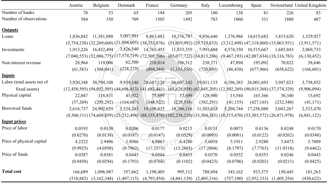
(28) 4. Data Description. This paper compiles unconsolidated accounting statements from the BankScope database of BVD-IBCA. The sample contains 1,303 commercial banks from 10 Western European countries, i.e., Austria, Belgium, Denmark, France, Germany, Italy, Luxembourg, Spain, Switzerland, and the United Kingdom, spanning 1996 to 2010. The data are scrutinized carefully in order to avoid potential inconsistency and keying errors. A several banks reporting extreme values on the variables of main interest are removed. The final unbalanced panel data contain 9,189 bank-year observations. Based on the intermediation approach, banks are assumed to hire three. 政治大 inputs—labor ( x ), physical capital ( x ), and borrowed funds ( x )—to produce three 立 1. 2. 3. ‧ 國. 學. outputs: total loans ( y1 ), other earning assets ( y2 ), and non-interest revenue ( y3 ). The output of non-interest revenue is used to reflect a bank’s degree of product. ‧. diversification, or equivalently, its degree of concentration on universal banking. y. Nat. n. al. er. io. banks.. sit. activities. This revenue constitutes a crucial source of income for modern universal. i Un. v. Because there are quite a few missing values on the number of employees, we. Ch. engchi. select the total assets net of fixed assets as the proxy for labor,3 and its price ( w1 ) is calculated as the ratio of personnel expenses to x1 . The input of physical capital is measured by the amount of fixed assets and its price ( w2 ) is measured by the ratio of other operating expenses to x2 . The input of borrowed funds consists of all deposits and borrowed money and its price ( w3 ) is defined as the ratio of total interest expenses to x3 . Total costs equal the sum of the three expenses. All of the inputs and 3. This selection is the same as Altunbaş et al. (2000, 2001b), Weill (2004), Fries and Taci (2005). 20.

(29) outputs are expressed in thousands of real US dollars deflated by the consumer price index of individual countries with base year 2000. Table 2 presents variable definitions. Table 3 summarizes the descriptive statistics for all variables and the detailed distribution of banks across countries. These statistics show that substantial variation in quantities of inputs and outputs and input prices exists among countries, implying that banks in these countries might adopt dissimilar production techniques and choose heterogeneous operation scales. Such differences justify the use of the metafrontier model for the study of international comparison.. 治政 The empirical analysis is conducted under a two-step 大 SF procedure, where the 立 effects of environmental heterogeneity on cost efficiency and TGR can be accounted ‧ 國. 學. for in both steps. Specifically, microeconomic variables explaining bank-specific. ‧. differences and macroeconomic variables reflecting country differences are included. sit. y. Nat. in the estimation of group frontiers and the metafrontier, respectively. The. io. er. micro-environmental variables in the first-step estimation of the group frontier in equation (3) are considered to be correlated with regulatory conditions, competitive. al. n. iv n C conditions, and ownership. The macro-environmental h e n g c h i U variables in the second-step. estimation of the metafrontier in equation (11) are considered to be associated with nationwide features that characterizing economic conditions and market structure as a whole. Table 4 summarizes those variables, along with related literature. In the first-step we estimate the FF cost frontier for each sample country. Three environmental variables are considered, i.e., equity to total assets ratio (ETA), average return on assets (ROA), and the ownership structure. To proxy for regulatory conditions faced by each country’s banking industry, the capital ratio, defined as the ratio of equity to total assets, is adopted. It is well-known that equity capital provides a buffer against portfolio losses and is regarded as a substitute for deposits and 21.

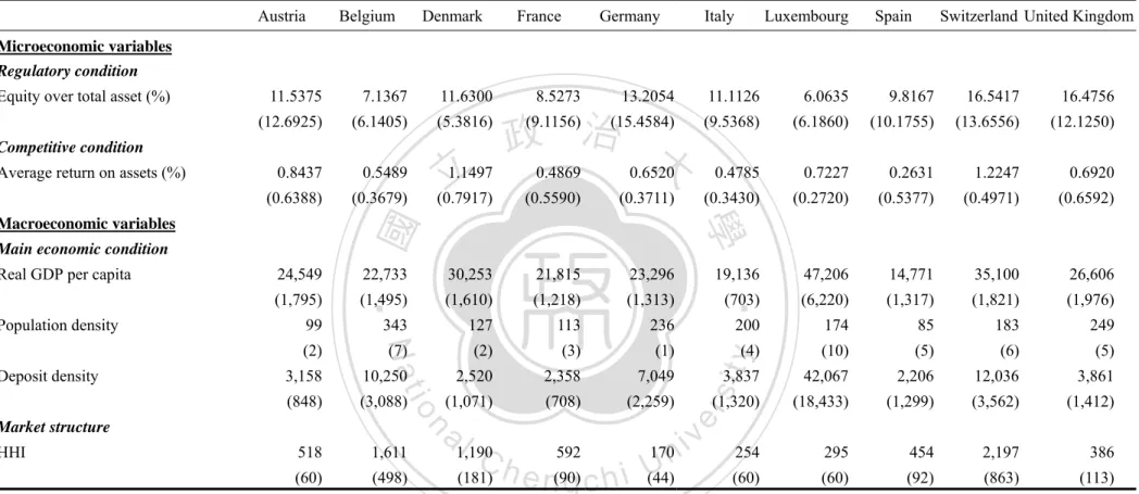
(30) Table 2 Summary of variables, descriptions, and data sources. Variables. Definition. Source. Total Loans ( y1 ). Short-term and long-term loans. Bankscope. Other earning assets ( y2 ). Other earning assets, including government bonds, corporate securities, and other investments Fee and commission income and other income. Input and output. Non-interest revenue ( y3 ). Bankscope Bankscope. Labor ( x1 ). Total assets (net of fixed assets). Bankscope. Physical capital ( x2 ). Total fixed assets. Bankscope. Borrowed funds ( x3 ). 政治大 Total personnel expenses / total assets. Bankscope. Deposits and borrowed money. Price of labor ( w1 ). 立. Bankscope Bankscope. Price of borrowed funds ( w3 ). Total interest expenses / total funding. Bankscope. ‧. ‧ 國. Other operating expenses / total fixed assets. 學. Price of physical capital ( w2 ). Microeconomic variables. Average ROA of all banks per annum. n. al. Domestic private banks. Bankscope. er. io. State-owned banks. y. Average return on assets. Bankscope. sit. The ratio of equity capital to total assets of a bank. Nat. Equity to asset ratio. State = 1 for state-owned banks and 0 otherwise; foreign banks are the normalization. Private = 1 for private banks and 0 otherwise; foreign banks are the normalization.. Ch. engchi. i Un. v. Bankscope. Bankscope. Macroeconomic variables. Real GDP per capita Population Density. The ratio of a nation’s real gross domestic WDI product to its population The ratio of inhabitants per square WDI kilometer. Deposit density. The ratio of deposit per square kilometer. IFS. HHI. The Herfindahl-Hirshmann index. ECB. Notes: WDI, World Development Indicator, World Bank; IFS, International Financial Statistics, IMF; ECB, EU Banking Structures, European Central Bank. 22.

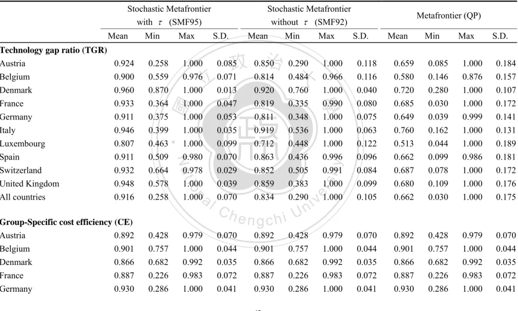
(31) Table 3 Summary statistics for banking costs, outputs, inputs, and input prices. Austria. Price of funds. Total cost. 1,329,927 (3,911,571) 2,069,733 (6,130,452) 58,646 (166,601). 3,920,348 30,794,108 9,939,146 28,687,128 26,607,142 19,011,135 6,196,383 26,001,693 3,947,823 (12,458,595) (94,052,505) (44,696,413) 141,683,441) 161,628,058) (62,845,205) (12,502,269) (90,015,368) (37,574,329) 22,047 118,831 41,922 75,699 57,699 128,980 15,544 165,366 30,340 (57,269) (295,292) (164,687) (348,922) (229,518) (382,291) (41,155) (427,165) (232,340) 2,616,737 24,902,029 5,524,243 19,108,835 18,766,116 11,503,018 5,204,744 17,256,080 3,043,267 (8,560,111) (74,669,859) (25,232,494) (88,335,476) (102,238,210) (33,504,383) (10,515,470) (53,385,572) (26,871,978). 3,758,852 (9,906,094) 15,692 (41,171) 2,533,470 (6,841,122). 0.0193 (0.0270) 4.2322 (9.9925) 0.0387 (0.0458). 0.0130 (0.0138) 2.9496 (4.0598) 0.0381 (0.0294). al. n. Price of physical capital. 1,836,842 11,381,888 5,007,991 8,863,882 10,376,787 9,856,646 1,376,986 14,615,682 1,815,620 (21,894,605) (5,754,238) (32,269,660) (38,733,876) (51,019,992) (29,710,833) (3,312,498) (47,318,860) (15,063,931) 1,913,226 16,432,494 3,826,540 14,765,455 11,833,355 7,991,604 4,574,350 10,515,667 1,685,843 (7,040,553) (52,086,775) (17,574,719) (72,505,596) (63,077,722) (34,813,286) (9,467,193) (42,087,634) (18,316,783) 62,500 28,964 119,006 218,014 196,312 238,371 47,894 195,092 70,822 (228,273) (61,583) (304,041) (894,384) (1,155,556) (720,893) (86,438) (677,966) (658,622). io. Input prices Price of labor. 83 487. 81 331. 政治大. Nat. Borrowed funds. 138 1060. Switzerland United Kingdom. ‧. fixed assets) Physical capital. 180 783. Spain. 學. Inputs Labor (total assets net of. 205 1492. Luxembourg. 226 1888. 立. 194 1505. Italy. y. Non-interest revenue. 65 709. Germany. sit. Investments. 53 350. France. 0.0206 (0.0187) 3.8986 (9.7962) 0.0443 (0.1793). 0.0177 (0.0147) 6.9867 (17.2573) 0.0504 (0.0768). Ch. 0.0215 (0.0529) 6.4280 (13.2885) 0.0453 (0.1102). engchi U. 166,689 1,096,987 357,662 1,198,405 (518,882) (3,162,348) (1,497,115) (4,793,454). er. Outputs Loans. 78 584. Denmark. ‧ 國. Number of banks Number of observations. Belgium. v 0.0151 i n (0.0093). 5.6058 (17.2804) 0.0370 (0.0423). 995,112 788,894 (4,841,139) (2,405,316). 0.0073 (0.0081) 5.1911 (8.1797) 0.0552 (0.0706). 0.0136 (0.0122) 2.9280 (7.7763) 0.0353 (0.0202). 0.0248 (0.0262) 3.8473 (11.9318) 0.0246 (0.0211). 0.0170 (0.0348) 5.7809 (9.6462) 0.0443 (0.0425). 343,162 933,575 150,445 (757,100) (2,952,333) (1,405,354). 181,263 (430,622). Notes: All inputs and outputs are expressed in thousands of real US dollars with a base year of 2000. Standard deviations are in parentheses. 23.

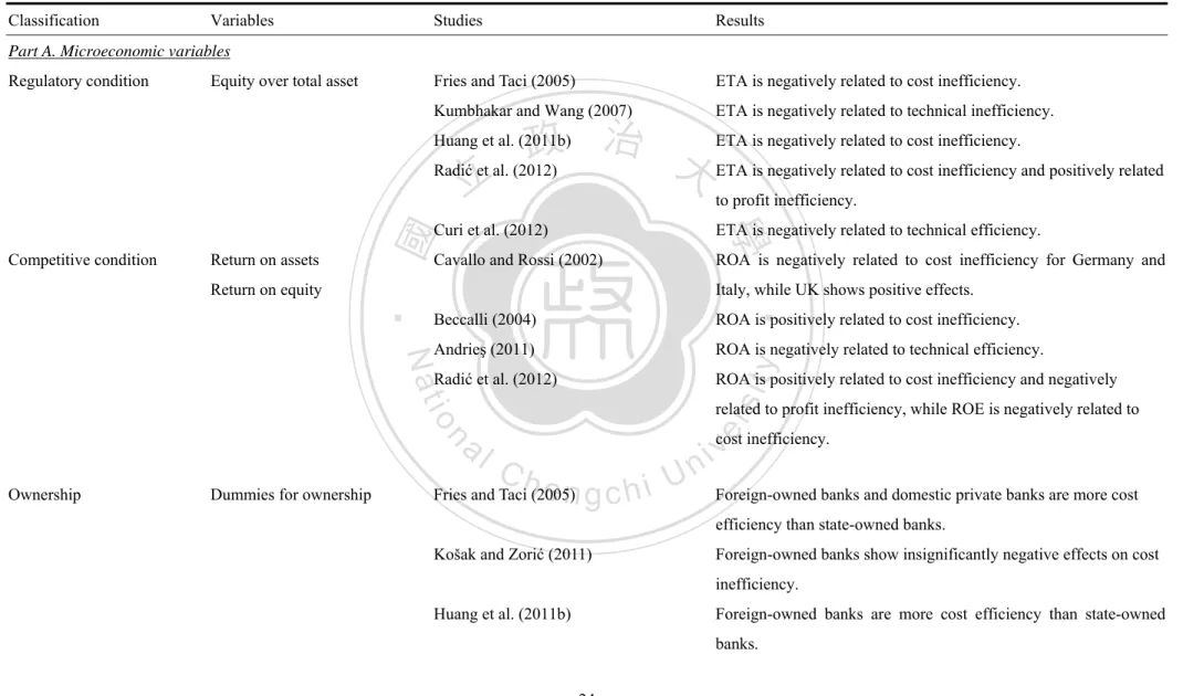
(32) Table 4 Listing of selected environmental variables used as determinants of efficiency in recent studies Classification. Variables. Studies. Results. Fries and Taci (2005). ETA is negatively related to cost inefficiency.. Kumbhakar and Wang (2007). ETA is negatively related to technical inefficiency.. Part A. Microeconomic variables Regulatory condition. Equity over total asset. 政治大 ETA is negatively related to cost inefficiency. Radić et al. (2012) ETA is negatively related to cost inefficiency and positively related 立 to profit inefficiency. Return on assets. ETA is negatively related to technical efficiency.. Cavallo and Rossi (2002). ROA is negatively related to cost inefficiency for Germany and Italy, while UK shows positive effects.. ‧. Return on equity. Curi et al. (2012). Beccalli (2004). ROA is positively related to cost inefficiency.. Andrieş (2011). ROA is negatively related to technical efficiency.. Radić et al. (2012). ROA is positively related to cost inefficiency and negatively related to profit inefficiency, while ROE is negatively related to. Dummies for ownership. v ni. cost inefficiency.. n. al. er. io. sit. y. Nat. Ownership. 學. Competitive condition. ‧ 國. Huang et al. (2011b). Ch. engchi U. Fries and Taci (2005). Foreign-owned banks and domestic private banks are more cost efficiency than state-owned banks.. Košak and Zorić (2011). Foreign-owned banks show insignificantly negative effects on cost inefficiency.. Huang et al. (2011b). Foreign-owned banks are more cost efficiency than state-owned banks. 24.

(33) Part B. Macroeconomic variables GDP per capita. condition. Radić et al. (2012). GDP per capita is negatively related to cost inefficiency and. PD shows insignificantly negative effects on cost inefficiency.. Košak and Zorić (2011). PD is positively related to cost inefficiency.. Radić et al. (2012). PD is positively related to cost inefficiency.. Dietsch and Lozano-Vivas (2000). DD is negatively related to banking costs. Huang et al. (2011b). DD is positively related to cost inefficiency.. Maudos et al. (2002). HHH is positively related to cost efficiency.. Andrieş (2011). HHH is positively related to technical efficiency.. y. sit. Košak and Zorić (2011). n. al. Ch. ‧. ‧ 國. Huang et al. (2011b). io. index. GDP per capita is negatively related to cost inefficiency.. 學. Herfindahl-Hirshmann. Košak and Zorić (2011). Nat. Market structure. GDP per capita is negatively related to cost inefficiency.. positively related to profit inefficiency. 治政 Curi et al. (2012) 大 GDP per capita is positively related to technical efficiency. 立 et al. (2010) Battaglia PD is negatively related to cost inefficiency.. Population density. Deposit density. Huang et al. (2011b). Radić et al. (2012). engchi. 25. er. Main economic. HHH is positively related to cost inefficiency.. v is positively related to cost and profit inefficiency. i HHH n U.

(34) borrowed money to finance loans. A bank with a lower equity level implies that its managers have a higher risk-taking attitude and are conducting a greater leverage. Hence, ETA is also referred to as a measure of a bank’s risk of insolvency. The higher the ETA, the lower is the insolvency risk. It is often claimed that the well-capitalized banks will be more efficient (Berger and Mester, 1997; Lozano-Vivas et al., 2001; Yildirim and Philippatos, 2007). The ROA is used as an indicator of a bank’s profitability that is intimately affected by the competitive condition of the banking industry. To proxy for competitive conditions encountered by each country’s banking industry, the average. 治政 return on assets in each year is calculated. In general, 大ROA reflects the ability of a 立 bank to generate profits by using its assets. According to Lozano-Vivas et al. (2001), ‧ 國. 學. Cavallo and Rossi (2002), Lozano-Vivas et al. (2002), and Andrieş (2011), the. ‧. relationship between the profitability ratio and efficiency is expected to be positive.. sit. y. Nat. The higher the profitability ratio is, the more efficient is the bank.. io. er. The relationship between ownership and efficiency has been one of the major research interests. Many efficiency studies emphasize the role of ownership in. al. n. iv n C assessing efficiency of banks. See,h for example, Beccalli e n g c h i U (2004), Bonin et al. (2005a,. b), Fries and Taci (2005), Yildirim and Philippatos (2007), Fang et al. (2011), Huang et al. (2011b), and Košak and Zorić (2011), to mention a few. As far as the corporate governance is concerned, different cost efficiency might be driven by ownership structures in the industry. As noted by Berger (2000), there are two main hypotheses pertaining to the effect of ownership. Under the home field advantage hypothesis, domestic private banks are more efficient than foreign-owned banks. Foreign-owned banks suffer from disadvantages, because they incur higher costs and receive lower revenues than domestic banks do. Conversely, under the global advantage hypothesis foreign-owned banks have competitive advantages over domestic banks, which results 26.

(35) in higher efficiency measures. The recent literature supports that foreign-owned banks operate more efficient than domestic private banks and state-owned banks. Our sample banks are classified into three ownership types, namely state-owned, domestic private, and foreign-owned banks, with the last one arbitrarily chosen as the normalization. In the second step, the new stochastic metafrontier model is formulated as the benchmark to evaluate the TGRs for each bank of all sample countries. The salient feature of the new model is its capability of linking the TGRs with a set of macroeconomic environmental variables, while the mixed model fails to do so. The. 治政 closer of group frontiers to the metafrontier means that 大the banking industry of that 立 country is inclined to undertake more advanced technology, and vice versa. Four ‧ 國. 學. environmental variables that are believed to influence the TGRs are included, i.e., real. sit. y. Nat. Herfindahl-Hirshmann index (HHI).4. ‧. GDP per capita (GDPPC), population density (PD), deposit density (DD), and. io. er. Variable GDPPC is measured by the ratio of a nation’s real gross domestic product to its population, serving as a proxy for the overall macroeconomic condition.. n. al. As noted by Dietsch and. iv n C Lozano-Vivas Lozano-Vivas h e n g c(2000), hi U. et al. (2001),. Lozano-Vivas et al. (2002), and Huang et al. (2011b), GDPPC affects both demand for and supply of banking services, such as deposits and loans. An increase in GDPPC raises the demand for loans and the supply of loanable funds fueled by savings, which may stimulate the bank profits and efficiency. In addition, a country with a higher level of GDPPC usually has developed a relatively mature banking system and operated under an advanced technology. Hence, the group frontiers of those countries tend to be closer to the matafrontier, corresponding to higher values of the TGR.. 4. The HHI is taken from the European Central Bank (ECB) annual report on EU banking structures. Switzerland is not included in the ECB report, whose HHI is directly computed from our data. 27.

(36) Population density (PD) is defined as the ratio of inhabitants per square kilometer. Lozano-Vivas et al. (2002) claim that a higher level of PD results in less expenditures on retail distribution of banking activities, which prompts bank efficiency. Conversely, the supply of banking services in a market of lower PD are likely to incur higher operating costs and little incentive to increase their efficiency (Radić et al., 2012). Thus, the relationship between the PD and TGRs is expected to be positive. Deposit density (DD) is calculated as the ratio of deposit per square kilometer. DD can have either positive or negative impacts on inefficiency. As noted by Fries and Taci (2005) and Weill (2007), DD has a negative influence on cost inefficiency,. 治政 as banks operating in a lower DD market would likely 大incur higher expenses. Banks 立 that are located in a country with higher level of DD might make the access to its ‧ 國. 學. business easier for customers. In this regard, it is expected that the gap between. ‧. country frontiers and the metafrontier is apt to shrink. On the contrary, Huang et al.. sit. y. Nat. (2011b) argue that banks operating in a market of high DD are facing keen. io. er. competition and have to employ more and higher quality inputs to provide high quality of services to their customers, but still charge competitive prices. As a result,. al. n. iv n C DD is anticipated to be positively h correlated i Uinefficiency. It is assumed the e n g c hwith higher the DD is, the wider is the gap between the country frontier and the metafrontier of the sample countries.. We select the measure of HHI to characterize the market structure of banking sectors, which is defined as the sum of squared market shares (multiplied by 100) of each bank in terms of total assets. The HHI ranges from 0 to 10,000. A value of HHI in excess of 1800 implies that the market is highly concentrated; a value of HHI lying between 1000 and 1800 indicates that the market’s degree of concentration is medium; while a value of HHI less than 1000 means that the market is highly competitive. The structure-conduct-performance (SCP) paradigm assumes that banks in countries with 28.

(37) lower market concentration are associated with higher level of market competition (Bain, 1951). One prediction of the SCP is that increased concentration should result in a decrease in efficiency, which is consistent with the quit life hypothesis (Hicks, 1935). Conversely, the efficiency structure hypothesis posits the opposite relationship, i.e., the efficient firms have lower cost and are able to increase their market share, which leads to higher concentration (Demsetz, 1974). Thus, market structure can have either positive or negative impacts on bank’s TGRs. Table 5 presents the descriptive statistics of all environmental variables used in both steps. These statistics display substantial heterogeneity in bank-specific and the. 治政 country characteristics. For instance, the ETA in 大 Austria, Denmark, Germany, 立 Switzerland, and the United Kingdom is much higher than other countries, indicating ‧ 國. 學. greater safety and soundness of the banking systems in these countries. With regard to. ‧. competitive condition, banks in Denmark and Switzerland earn higher ROA than. sit. y. Nat. other countries. As for macro-conditions the real GDP per capita in Denmark,. io. er. Luxembourg, and Switzerland leads the remaining countries, while Belgium, Luxembourg, and Switzerland have higher population density and deposit density.. n. al. Finally, Switzerland has a. Ch highly. econcentrated ngchi. iv n financial U. market, Belgium and. Denmark have moderately concentrated financial market, and the remaining countries have relatively competitive financial market. The foregoing statistics uncover that banks in different countries have different features, caused mainly by distinct regulatory environments, managerial abilities, economic environments, economic development, and market structure. Given these fundamental differentiations, it is critical to take them into account in the efficiency assessment and comparison among distinct groups operating under heterogeneous technologies. This justifies the use of the new metafrontier model that enables the calculation of comparable cost efficiencies to be linked with those determinants for 29.

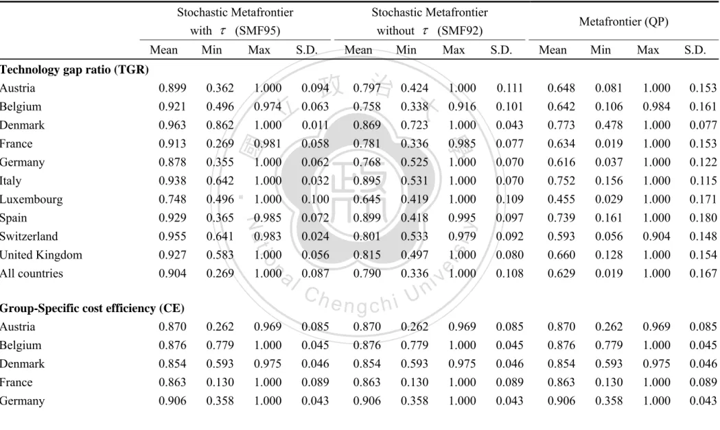
(38) Table 5 Summary statistics for environmental variables. Austria. Belgium. Denmark. France. Germany. Italy. Luxembourg. Spain. Switzerland United Kingdom. Microeconomic variables 11.5375. 7.1367. 11.6300. (12.6925). (6.1405). (5.3816). 0.8437. 0.5489. (0.6388). (0.3679). 1.1497 立 (0.7917). 24,549. Competitive condition Average return on assets (%). 16.4756. (9.5368). (6.1860). (10.1755). (13.6556). (12.1250). 0.4785. 0.7227. 0.2631. 1.2247. 0.6920. (0.3430). (0.2720). (0.5377). (0.4971). (0.6592). 21,815. 23,296. 19,136. 47,206. 14,771. 35,100. 26,606. (1,218). (1,313). (703). (6,220). (1,317). (1,821). (1,976). 343. 127. 113. 236. 200. 174. 85. 183. 249. (7). (2). (3). (1). (4). y. (10). (5). (6). (5). 3,158. 10,250. 2,520. 2,358. 7,049. 3,837. 42,067. 2,206. 12,036. 3,861. (848). (3,088). (1,071). (708). (2,259). (1,320). (18,433). (1,299). (3,562). (1,412). 518. 1,611. 254. 295. 454. 2,197. 386. (60). (498). (60). (60). (92). (863). (113). 99. Nat. 30,253 (1,610). io. al. n. Market structure HHI. 16.5417. 22,733. (2) Deposit density. (0.3711). 9.8167. (1,495). (1,795) Population density. (0.5590). 6.0635. ‧. Real GDP per capita. (9.1156) (15.4584) 政治大 0.4869 0.6520. 11.1126. sit. Main economic condition. 13.2054. 學. Macroeconomic variables. 8.5273. Ch. 1,190. (181). 592. e n(90) gchi. er. Equity over total asset (%). ‧ 國. Regulatory condition. i n U 170. (44). v. Notes: Real GDP per capita and deposit density are expressed in thousands of real US dollars with a base year of 2000. Standard deviations are in parentheses.. 30.

(39) banks in different nations. Figures A1-A10, Appendix A, provide graphical representations for the correlation matrix among the explanatory variables for each country frontier in the first-step estimation. The pairwise correlation coefficients are shown in the lower triangle, while elements in the upper triangle draw the correlation coefficients by using circular encodings. Generally speaking, the degrees of correlations between explanatory variables, except for the output variables, are generally weak, which excludes the collinear problem among explanatory variables. As for the metafrontier in the second-step estimation, Figure A11 also presents a graphical correlation matrix.. 治政 Most of these coefficients are significant, but their signs 大 are different. As far as the 立 various macroeconomic environmental conditions are concerned, the highest ‧ 國. 學. correlation coefficient between real GDP per capita and deposit density is 0.84, while. ‧. the lowest is -0.01 between deposit density and Herfindahl-Hirshmann index. The. sit. y. Nat. remaining correlation coefficients are generally low ranged from 0.03 to 0.27, which. io. n. al. er. preclude the existence of the collinear problem among these variables.. Ch. engchi. 31. i Un. v.

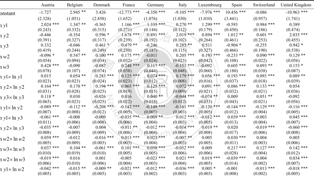
(40) 5. Empirical Results and Analysis. This section presents all of our empirical results. In the first subsection we show the parameter estimates of the stochastic cost frontier for both the FF and the translog functional forms, and perform some hypothesis tests for each country. In the second subsection we analyze implications drawn from the estimated cost efficiency scores and the TGRs. The third subsection aims to provide a detailed discussion on the trending of various efficiency measures during the sample period. Finally, some further evidence about the impact of a bank’s size, profitability, and risk attitude on the efficiencies is investigated.. 5.1 Parameter Estimates. 立. 政治大. ‧ 國. 學. Software FRONTIER 4.1 (see Coelli, 1996) is applied to yield the parameter. ‧. estimates for all of the 10 country frontiers of Equation (1). Both the FF and the. sit. y. Nat. standard translog cost functions are estimated for the purpose of comparison. Table 6. io. er. merely summarizes the translog part of the parameter estimates of the FF cost function for each country and the estimates of Fourier series are shown in Table B1 of. al. n. iv n C Appendix B. Table B2 presents thehestimation resultsUof the translog cost function. It engchi. is seen that more than half of the parameter estimates in each country reach statistical. significance at least at the 10% level. The hypothesis that the parameters of all the Fourier series are joint zero is decisively rejected at the 1% level of significance by the likelihood ratio (LR) test. We, thus, claim that the FF cost function is valid to represent the sample banks’ production technologies and the underlying cost structure. As far as the environmental conditions are concerned, Table 7 summarizes coefficient estimates of the micro-level environmental variables based on the FF cost function. The outcomes reveal that most of those estimates are significant in each sample country, but their signs are different, caused possibly by the distinct 32.

(41) Table 6 Parameter estimates of the Fourier flexible cost frontier for the sample countries. ln y 3. ln w2 ln y1× ln y1. ln y1× ln y 2. ln w2 × ln w2 ln w3 × ln w3 ln w2 × ln w3 ln y1 × ln w2. -9.105 *** (1.030) 0.270 ** (0.112) 2.019 *** (0.102) 0.285 ** (0.115) 0.205 *** (0.023) -0.151 *** (0.048) 0.179 *** (0.008) 0.072 *** (0.009) -0.044 *** (0.012) -0.161 *** (0.003) 0.012 *** (0.003) -0.014 *** (0.004) -0.007 ** (0.003) -0.052 *** (0.006) 0.021 *** (0.004) -0.036 *** (0.003). -7.976 *** (1.010) 1.299 *** (0.179) 0.894 *** (0.264) 0.511 (0.327) 0.193 *** (0.042) -0.092 (0.060) 0.056 *** (0.016) 0.091 *** (0.021) -0.074 ** (0.033) -0.120 *** (0.005) -0.012 *** (0.005) 0.019 ** (0.008) 0.005 (0.005) 0.009 (0.006) 0.019 *** (0.005) 0.005 * (0.003). 立. 政治大. al. n. ln y 2 × ln y3. -4.350 *** (1.076) 1.335 *** (0.144) 0.891 *** (0.192) -0.246 (0.187) -0.011 (0.024) 0.117 *** (0.044) 0.074 *** (0.012) 0.125 *** (0.015) 0.040 ** (0.018) -0.149 *** (0.003) 0.009 ** (0.004) -0.012 *** (0.004) 0.023 *** (0.004) 0.058 *** (0.005) -0.023 *** (0.003) -0.012 *** (0.002). io. ln y1× ln y3. -12.773 *** (1.652) 1.166 *** (0.271) 1.678 *** (0.239) 0.479 ** (0.230) 0.175 *** (0.032) 0.248 *** (0.038) 0.125 *** (0.023) 0.065 *** (0.019) 0.016 (0.022) -0.142 *** (0.005) -0.035 *** (0.006) -0.011 ** (0.006) 0.013 *** (0.003) 0.101 *** (0.005) -0.005 (0.004) -0.021 *** (0.003). Nat. ln y 3 × ln y 3. Luxembourg. Ch. engchi. 33. ‧. ln y 2 × ln y 2. Italy. 學. ln w3. 3.426 (2.858) -0.365 (0.315) 0.596 * (0.317) 0.461 * (0.249) 0.100 *** (0.034) -0.087 (0.074) 0.283 *** (0.024) 0.194 *** (0.025) -0.026 (0.025) -0.208 *** (0.012) -0.009 (0.008) 0.004 (0.009) -0.016 *** (0.003) -0.061 *** (0.010) 0.001 (0.006) -0.009 ** (0.005). Germany. y. ln y 2. 2.945 ** (1.051) 1.347 ** (0.332) -0.354 (0.327) -0.046 (0.244) 0.547 ** (0.094) -0.090 (0.107) 0.054 ** (0.023) 0.170 ** (0.028) 0.030 (0.023) -0.112 ** (0.008) -0.008 (0.006) -0.007 (0.009) -0.012 (0.009) 0.104 ** (0.019) 0.016 (0.010) -0.015 ** (0.005). France. sit. ln y1. -1.727 (2.328) 2.024 *** (0.243) -0.446 (0.391) 0.332 (0.419) -0.096 * (0.054) 0.428 *** (0.078) 0.015 (0.023) 0.164 *** (0.031) 0.118 * (0.065) -0.089 *** (0.007) -0.061 *** (0.011) -0.035 *** (0.008) 0.059 *** (0.005) 0.037 *** (0.010) -0.019 *** (0.006) -0.042 *** (0.005). Denmark. er. constant. Belgium. ‧ 國. Austria. i n U. v. Spain 10.456 *** (3.441) -0.593 (0.450) 1.012 ** (0.461) -0.904 * (0.466) -0.233 ** (0.108) 0.605 *** (0.180) 0.193 *** (0.037) 0.086 *** (0.032) 0.009 (0.043) -0.144 *** (0.012) 0.039 *** (0.013) 0.020 (0.017) 0.030 *** (0.011) 0.217 *** (0.028) -0.039 *** (0.014) -0.001 (0.008). Switzerland. United Kingdom. -0.086 (0.957) 0.984 *** (0.186) 0.601 ** (0.253) -0.255 (0.190) 0.090 *** (0.022) 0.093 ** (0.038) 0.093 *** (0.018) 0.133 *** (0.021) 0.051 ** (0.021) -0.129 *** (0.004) -0.003 (0.004) -0.019 *** (0.006) 0.004 (0.003) 0.127 *** (0.004) 0.004 (0.002) -0.013 *** (0.002). -10.963 *** (1.741) 0.389 (0.474) 2.035 *** (0.455) 0.942 * (0.538) 0.129 ** (0.056) 0.153 * (0.087) 0.089 ** (0.039) 0.054 (0.036) -0.092 (0.056) -0.116 *** (0.005) 0.045 *** (0.007) -0.060 *** (0.008) 0.005 (0.006) 0.142 *** (0.012) 0.034 *** (0.007) -0.018 *** (0.005).

比較西歐銀行業之成本效率： 新共同邊界Fourier成本函數之應用 - 政大學術集成

比較西歐銀行業之成本效率：新共同邊界Fourier成本函數之應用 - 政大學術集成