完全多部圖之線性k蔭度

全文

(1)國立交通大學應用數學系博士論文完全多部圖之線性 k 蔭度 Linear k-arboricity of Complete Multipartite Graphs. 研究生：嚴志弘指導教授：傅恆霖教授. 中華民國九十四年六月.

(2) 完全多部圖之線性 k 蔭度 Linear k-arboricity of Complete Multipartite Graphs. 研究生：嚴志弘. Student：Chih-Hung Yen. 指導教授：傅恆霖教授. Advisor：Professor Hung-Lin Fu. 國立交通大學應用數學系博士論文. A Dissertation Submitted to Department of Applied Mathematics College of Science National Chiao Tung University in Partial Fulfillment of the Requirements for the Degree of Doctor of Philosophy in Applied Mathematics June 2005 Hsinchu, Taiwan, Republic of China. 中華民國九十四年六月.

(3) 完全多部圖之線性 k 蔭度研究生：嚴志弘. 指導教授：傅恆霖教授. 國立交通大學應用數學系. 摘. 要. 如果圖形 G 的一些子圖能讓 G 的每一個邊恰好只出現在它們的其中之一，則這些子圖被稱為是圖形 G 的一個分解。到目前為止，在圖形的分解這個研究領域上，已經有不少有趣的結果和問題被發表。而這篇論文所要探討的是其中的一個問題，我們稱做是線性 k 蔭度問題。一個完全由長度不大於 k 的路徑所構成的圖形，我們稱之為線性 k 森林。而一個圖形 G 所能分解成線性 k 森林的最少數量則稱為圖形 G 的線性 k 蔭度。因此，當一個圖形給定後，它的線性 k 蔭度為何，就是我們所謂的線性 k 蔭度問題。對於線性 k 蔭度所闡述的概念，我們可以將之視為圖形理論裡邊著色課題的一種延伸性想法，以及對線性蔭度課題更深入詳盡的探究。而所謂的線性蔭度，其實是將線性 k 蔭度的定義裡有關於路徑長度的限制去除。在西元 1982 年，針對一個圖形 G 的線性 k 蔭度的上界，有兩位學者提出了一個重要猜測。而對於這個猜測的驗證，迄今也發表了許多的結果在文獻裡。譬如當圖形 G 是一個立方圖、一個樹、一個完全圖、或者是一個均衡完全二部圖，以及某些特定的 k 值。在這篇論文裡，我們會確定均衡完全二部圖、完全圖、和部份的均衡完全多部圖的線性 3 蔭度。同時，對於部份的完全二部圖、完全圖、和均衡完全多部圖，我們也會提供它們的線性 2 蔭度的值。而所有我們獲得的結果，在相同的條件下，會剛好驗證上述的猜測。此外，在這篇論文裡，我們還探討了一個關於位元排列網路的問題。我們會證明從一個位元排列網路N的有向線圖所建構出的新網路G(N)+，它的結構將依然是一個位元排列網路。我們也會給定一個簡易的運算式，它能夠從N的特徵向量 + 來導出G(N) 的特徵向量。這個運算式可以幫助我們去獲得位元排列網路彼此之間的關聯性。 i.

(4) Linear k-arboricity of Complete Multipartite Graphs Student: Chih-Hung Yen. Advisor: Professor Hung-Lin Fu. Department of Applied Mathematics. Department of Applied Mathematics. National Chiao Tung University. National Chiao Tung University. Abstract A decomposition of a graph is a list of subgraphs such that each edge appears in exactly one subgraph in the list. There are many interesting results and problems in this area. In this thesis, we study a special case of graph decomposition, called the linear k-arboricity problem. A linear k-forest is a graph whose components are paths with lengths at most k. The minimum number of linear k-forests needed to decompose a graph G is the linear k-arboricity of G, denoted lak (G). Thus, the linear k-arboricity problem is what the value lak (G) should be when a graph G is given. The notion of linear k-arboricity is a natural generalization of edge coloring and also a refinement of the concept of linear arboricity in which the paths have no length constraints. In 1982, Habib and Peroche made the following conjecture: Conjecture. If G is a graph with maximum degree ∆(G) and k ≥ 2, then  » ¼  ∆(G)·|V (G)|  if ∆(G) = |V (G)| − 1 and  (G)|  c  2b k·|Vk+1 lak (G) ≤ ¼ »    ∆(G)·|V (G)|+1  if ∆(G) < |V (G)| − 1.  k·|V (G)| 2b k+1 c So far, in the literature, quite a few results on the verification of this conjecture have been obtained. For example, when G is a cubic graph, tree, complete graph, or e − 1. balanced complete bipartite graph, and k is small or k ≥ d |V (G)| 2 ii.

(5) In this thesis, we determine the linear 3-arboricity of balanced complete bipartite graphs, complete graphs, and parts of balanced complete multipartite graphs. We also give some substantial results about the linear 2-arboricity of complete bipartite graphs, complete graphs, and balanced complete multipartite graphs. The results obtained are coherent with the corresponding cases of the conjecture mentioned above. Furthermore, in this thesis, we study a problem on the bit permutation network. We prove that if N is an s-stage d-nary bit permutation network with dn inputs (outputs), then a new network L(N )+ obtained from the line digraph of N is an (s + 1)-stage d-nary bit permutation network with dn+1 inputs (outputs). We also give a simple (but not trivial) formula to determine the characteristic vector of L(N )+ from the characteristic vector of N . This formula can help us to obtain relations between some well-studied bit permutation networks.. iii.

(6) Acknowledgments I want to offer my heartfelt thanks to everyone that ever helped me to finish the thesis of my doctor’s degree. My advisor, Professor Hung-Lin Fu, provided me with expert guidance, many hours of discussion, and financial support to complete the thesis. I am grateful for all that he had done. I am thankful to all members of the committee: Professor Ko-Wei Lih, Professor Xuding Zhu, Professor Yeong-Nan Yeh, Professor Bor-Liang Chen, Professor KuoChing Huang, Professor Chiuyuan Chen, and Professor Chih-Wen Weng. Thanks to them for suggesting many thoughtful improvements. Special thanks to Professor Frank Kwang-Ming Hwang, Professor Bor-Liang Chen, Professor Kuo-Ching Huang, Professor Chiuyuan Chen, and Professor Chikaung Pai for sharing their experiences on real life and research. I wish to thank many friends: Ming-Hway Huang, Jun-Jie Pan, Yu-Chung Chang, You-Bin Cao, Bey-Chi Lin, Chia-Fen Chang, Hung-Song Hseu, Jyh-Min Kuo, KaiChung Cheng, Chi-Ming Liao, Mei-Jing Tzeng, Qi-Xian Liu and so on. With whom I had many discussions not only about mathematics. To my parents, wife and the other members in my family, I felt an immense gratitude for their infinite support throughout all stages of my life.. iv.

(7) Contents Abstract (in Chinese). i. Abstract (in English). ii. Acknowledgements. iv. Contents. v. List of Figures. vii. 1 Fundamental Concepts. 1. 1.1. Graphs . . . . . . . . . . . . . . . . . . . . . . . . . . . . . . . . . . .. 1. 1.2. Directed Graphs . . . . . . . . . . . . . . . . . . . . . . . . . . . . . .. 4. 1.3. Special Types of Graphs . . . . . . . . . . . . . . . . . . . . . . . . .. 7. 1.4. Switching Networks . . . . . . . . . . . . . . . . . . . . . . . . . . . .. 9. 1.5. Overview . . . . . . . . . . . . . . . . . . . . . . . . . . . . . . . . . .. 12. 2 The Linear k-arboricity Problem. 13. 2.1. Introduction . . . . . . . . . . . . . . . . . . . . . . . . . . . . . . . .. 13. 2.2. The Known Results . . . . . . . . . . . . . . . . . . . . . . . . . . . .. 15. 3 Linear 3-arboricity of Balanced Complete Multipartite Graphs. 18. 3.1. Preliminary Lemmas . . . . . . . . . . . . . . . . . . . . . . . . . . .. 18. 3.2. Balanced Complete Bipartite Graphs . . . . . . . . . . . . . . . . . .. 20. 3.3. Complete Graphs . . . . . . . . . . . . . . . . . . . . . . . . . . . . .. 24. 3.4. Balanced Complete Multipartite Graphs . . . . . . . . . . . . . . . .. 36. v.

(8) 4 Linear 2-arboricity of Complete Multipartite Graphs. 44. 4.1. Complete Bipartite Graphs . . . . . . . . . . . . . . . . . . . . . . . .. 44. 4.2. Complete Graphs . . . . . . . . . . . . . . . . . . . . . . . . . . . . .. 46. 4.3. Balanced Complete Multipartite Graphs . . . . . . . . . . . . . . . .. 53. 5 Bit Permutation Networks. 57. 5.1. Introduction . . . . . . . . . . . . . . . . . . . . . . . . . . . . . . . .. 57. 5.2. Preliminary Lemmas . . . . . . . . . . . . . . . . . . . . . . . . . . .. 59. 5.3. The Main Results . . . . . . . . . . . . . . . . . . . . . . . . . . . . .. 64. 6 Conclusion. 68. Bibliography. 70. vi.

(9) List of Figures 1.1. A drawing of a finite simple graph. . . . . . . . . . . . . . . . . . . .. 2. 1.2. A subgraph of the graph in Figure 1.1. . . . . . . . . . . . . . . . . .. 3. 1.3. A digraph D. . . . . . . . . . . . . . . . . . . . . . . . . . . . . . . .. 5. 1.4. A digraph D and its underlying graph G. . . . . . . . . . . . . . . . .. 6. 1.5. A balanced complete bipartite graph K2,2 . . . . . . . . . . . . . . . .. 7. 1.6. G and its line graph L(G); D and its line digraph L(D). . . . . . . .. 8. 1.7. A 3-stage MIN. . . . . . . . . . . . . . . . . . . . . . . . . . . . . . .. 11. 1.8. The line digraph of the network in Figure 1.7. . . . . . . . . . . . . .. 11. 2.1. Two linear 3-forests in K4 . . . . . . . . . . . . . . . . . . . . . . . . .. 13. 3.1. A 1-factorization of K4 .. . . . . . . . . . . . . . . . . . . . . . . . . .. 19. 3.2. Two linear 3-forests in K6,6 . . . . . . . . . . . . . . . . . . . . . . . .. 20. 3.3. The array shows that la3 (K6,6 ) ≤ 4. . . . . . . . . . . . . . . . . . . .. 21. 3.4. Two linear 3-forests and one isolated edge in K7,7 . . . . . . . . . . . .. 22. 3.5. The array shows that la3 (K7,7 ) ≤ 5. . . . . . . . . . . . . . . . . . . .. 22. 3.6. A linear 3-forest in K8 . . . . . . . . . . . . . . . . . . . . . . . . . . .. 25. 3.7. Two linear 3-forests in K8 . . . . . . . . . . . . . . . . . . . . . . . . .. 26. 3.8. The array shows that la3 (K8 ) ≤ 5.. . . . . . . . . . . . . . . . . . . .. 26. 3.9. A linear 3-forest in K10 . . . . . . . . . . . . . . . . . . . . . . . . . .. 27. 3.10 Another linear 3-forest in K10 . . . . . . . . . . . . . . . . . . . . . . .. 28. 3.11 The process of replacing the paths of length 3. . . . . . . . . . . . . .. 31. 3.12 The array shows four linear 3-forests in G(X, Y ). . . . . . . . . . . .. 33. 3.13 A linear 3-forest in K35 . . . . . . . . . . . . . . . . . . . . . . . . . .. 35. vii.

(10) 4.1. An example of a symmetric PILS(8; 2, 2, 2, 2). . . . . . . . . . . . . .. 47. 4.2. The array shows that la2 (K11 ) ≤ 8. . . . . . . . . . . . . . . . . . . .. 48. 4.3. The array shows that la2 (K12 − {v1 v4 , v6 v10 , v7 v11 }) ≤ 8. . . . . . . .. 48. 4.4. The symmetric array shows that la2 (K35 ) ≤ 26. . . . . . . . . . . . .. 49. 4.5. The array shows that la2 (K12,12 ) ≤ 9. . . . . . . . . . . . . . . . . . .. 50. 4.6. The array shows that la2 (K11,12 ∪ G[{v1 v4 , v6 v10 , v7 v11 }]) ≤ 9. . . . . .. 51. 4.7. Four subarrays of the array in Figure 4.4. . . . . . . . . . . . . . . . .. 52. 4.8. A (12t + 11) × (12t + 11) symmetric array. . . . . . . . . . . . . . . .. 53. 4.9. Three linear 2-forests in K3(7) . . . . . . . . . . . . . . . . . . . . . . .. 54. 5.1. A bit permutation network N2 (4; u, v, f1 , f2 , f3 ). . . . . . . . . . . . .. 58. 5.2. A bit permutation network N2 (4; I3 , I1 , I2 ). . . . . . . . . . . . . . . .. 59. 5.3. The line digraph L(N ) obtained from the network in Figure 5.1. . . .. 60. 5.4. The network L(N )+ obtained from the network in Figure 5.1. . . . .. 61. 5.5. The network BYF (1, 4). . . . . . . . . . . . . . . . . . . . . . . . . . .. 66. viii.

(11) Chapter 1 Fundamental Concepts In this chapter, we shall list the basic notations, terminologies, and definitions on graph theory and the mathematical theory of switching networks, which are the excerpts from two textbooks, one by Douglas B. West [28] and the other by Frank K. Hwang [16]. We also give an overview of this thesis.. 1.1. Graphs. A graph G is a triple consisting of a vertex set V (G), an edge set E(G), and a relation that associates with each edge two vertices (not necessarily distinct) called its endpoints. We draw a graph on paper by placing each vertex at a point and representing each edge by a curve joining the locations of its endpoints. A loop is an edge whose endpoints are equal. Multiple edges are edges having the same pair of endpoints. A simple graph is a graph having no loops or multiple edges. In this case an edge is determined by its endpoints, so we can view an edge as an unordered pair of vertices. Thus a simple graph can be specified by its vertex set and edge set, treating the edge set as a set of unordered pairs of vertices and writing e = uv (or e = vu) for an edge e with endpoints u and v. The order of a graph G, written |V (G)|, is the number of vertices in G. The size of a graph G, written |E(G)|, is the number of edges in G. A graph G is finite if its vertex set and edge set are finite, i.e., |V (G)| and |E(G)| are well-defined nonnegative integers. The null graph is the graph whose vertex set and edge set are empty.. 1.

(12) Figure 1.1 is a drawing of a finite simple graph. The vertex set is {u, v, w, x, y}, and the edge set is {uv, uw, ux, vx, vw, xw, xy}. v. w. u u @ ¡ @ ¡ ¡ @u u. u. x. u. y. Figure 1.1: A drawing of a finite simple graph.. We adopt the convention that every graph mentioned in this thesis is finite and simple. Besides, all statements should be considered only for graphs with a nonempty set of vertices. If vertex v is an endpoint of edge e, then v and e are incident. The degree of vertex v in a loopless graph G, written dG (v), is the number of edges incident to v. The maximum degree is ∆(G) and the minimum degree is δ(G). A vertex is odd (even) when its degree is odd (even). An isolated vertex is a vertex of degree 0. When u and v are the endpoints of an edge, they are adjacent and are neighbors. The neighborhood of v in G, written NG (v), is the set of vertices adjacent to v. Furthermore, two edges are incident if they have one endpoint in common. A matching in a graph G is a set of non-loop edges with no shared endpoints. The vertices incident to the edges of a matching M are saturated by M ; the others are unsaturated (we say M -saturated and M -unsaturated). A perfect matching in a graph is a matching that saturates every vertex. A matching is a set of edges, so its size is the number of edges. A k-edge-coloring of a graph G is a labelling f : E(G) → S, where |S| = k. The labels are colors; the edges of one color form a color class. A k-edge-coloring is proper if incident edges have different labels; that is, if each color class is a matching. A graph is k-edge-colorable if it has a proper k-edge-coloring. The chromatic index χ0 (G) of a graph G is the least k such that G is k-edge-colorable. A subgraph of a graph G is a graph H such that V (H) ⊆ V (G), E(H) ⊆ E(G), and the assignment of endpoints to edges in H is the same as in G, written H ⊆ G. 2.

(13) For example, the graph in Figure 1.2 is a subgraph of the graph in Figure 1.1. v u u. u. u. x. u. y. Figure 1.2: A subgraph of the graph in Figure 1.1.. A path is a simple graph whose vertices can be ordered so that two vertices are adjacent if and only if they are consecutive in the list. A cycle is a graph with an equal number of vertices and edges whose vertices can be placed around a circle so that two vertices are adjacent if and only if they appear consecutively along the circle. The path and cycle with n vertices are denoted Pn and Cn , respectively; an n-cycle is a cycle with n vertices. A cycle Cn is odd (even) when n is odd (even). A path in a graph G is a subgraph of G that is a path (similarly for cycles). A walk is a list v0 , e1 , v1 , . . . , ek , vk of vertices and edges such that, for 1 ≤ i ≤ k, the edge ei has endpoints vi−1 and vi . A trail is a walk with no repeated edges. A u, v-walk or u, v-trail has first vertex u and last vertex v; these are its endpoints. A u, v-path is a path whose vertices of degree 1 (its endpoints) are u and v; the others are internal vertices. The length of a walk, trail, path, or cycle is its number of edges. In a simple graph, a walk (or trail) is completely specified by its ordered list of vertices. We usually name a path, cycle, trail, or walk in a simple graph by listing only its vertices in order, even though it consists of both vertices and edges. A graph G is connected if it has a u, v-path whenever u, v ∈ V (G) (otherwise, G is disconnected). If G has a u, v-path, then u is connected to v in G. A maximal connected subgraph of G is a subgraph that is connected and is not contained in any other connected subgraph of G. The components of a graph G are its maximal connected subgraphs. Components are pairwise disjoint; no two share a vertex. A component (or a graph) is trivial if it has no edges; otherwise it is nontrivial.. 3.

(14) We write G − e or G − M for the subgraph of G obtained by deleting an edge e or a set of edges M . We write G − v or G − S for the subgraph obtained by deleting a vertex v or a set of vertices S. Note that when we obtain a subgraph by deleting a vertex, it must be a graph, so deleting the vertex also deletes all edges incident to it. Suppose that V 0 ⊆ V (G) and E 0 ⊆ E(G). The subgraph of G induced by V 0 , written G[V 0 ], is the subgraph of G consists of V 0 as its vertex set and all edges in G whose endpoints are contained in V 0 . Similarly, the subgraph of G induced by E 0 , written G[E 0 ], is the subgraph of G consists of E 0 as its edge set and all vertices in G which are the endpoints of edges in E 0 . We say that G[V 0 ] is an induced subgraph of G and G[E 0 ] is an edge-induced subgraph of G. The union of graphs G1 , G2 , . . . , Gk , written G1 ∪ G2 ∪ · · · ∪ Gk , is the graph S S with vertex set ki=1 V (Gi ) and edge set ki=1 E(Gi ). When a graph G is expressed as the union of two or more subgraphs, an edge of G can belong to many of them. If any edge in the union G of G1 , G2 , . . . , Gk is contained only by one of G1 , G2 , . . . , Gk , then we say G is an edge-disjoint union. If G and H are two graphs with disjoint vertex sets, then the graph obtained by taking the union of G and H is the disjoint union or sum, written G + H.. 1.2. Directed Graphs. In general, a relation on S can be any set of ordered pairs in S × S. For such relations, we need a more general model. A directed graph or digraph D is a triple consisting of a vertex set V (D), an edge set E(D), and a function assigning each edge an ordered pair of vertices. The first vertex of the ordered pair is the tail of the edge, and the second is the head; together, they are the endpoints. The terms “head” and “tail” come from the arrows used to draw digraphs. As with graphs, we assign each vertex a point in the plane and each edge a curve joining its endpoints. When drawing a digraph, we give the curve a direction from the tail to the head. Figure 1.3 shows a digraph D with vertex set V (D) = {a, b, c, d, e, f } and edge set E(D) = {(a, b), (b, c), (c, d), (d, e), (e, a), (f, a)}.. 4.

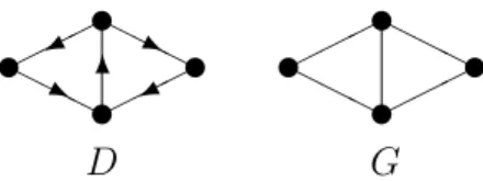
(15) d. u ¡@ e ¡ ª @ I c ¡ @u u ? u- u. f. -. a. 6 u. b. Figure 1.3: A digraph D.. When a digraph models a relation, each ordered pair is the (head, tail) pair for at most one edge. In this setting as with simple graphs, we ignore the technicality of a function assigning endpoints to edges and simply treat an edge as an ordered pair of vertices. In a digraph, a loop is an edge whose endpoints are equal. Multiple edges are edges having the same ordered pair of endpoints. A digraph is simple if each ordered pair is the head and tail of at most one edge; one loop may be present at each vertex. In a simple digraph, we write uv for an edge with tail u and head v. If there is an edge from u to v, then v is a successor of u, and u is a predecessor of v. We write u → v for “there is an edge from u to v”. A digraph is a path if it is a simple digraph whose vertices can be linearly ordered so that there is an edge with tail u and head v if and only if v immediately follows u in the vertex ordering. A cycle is defined similarly using an ordering of the vertices on a circle. We often use the same names for corresponding concepts in the graph and digraph models. Also, a graph G can be modelled using a digraph D in which each edge uv ∈ E(G) is replaced with uv, vu ∈ E(D). In this way, results about digraphs can be applied to graphs. Since the notion of “edge” in digraphs extends the notion of “edge” in graphs, using the same name makes sense. The underlying graph of a digraph D is the graph G obtained by treating the edges of D as unordered pairs; the vertex set and edge set remain the same, and the endpoints of an edge are the same in G as in D, but in G they become an unordered pair. Figure 1.4 shows a digraph D and its underlying graph G. 5.

(16) u ©©HHH © u ©u HH © H© u. u ¼©Hj © HHu © u Hj 6 ¼© © HH© u. G. D. Figure 1.4: A digraph D and its underlying graph G.. The definitions of subgraph and union are the same for graphs and digraphs. A digraph is weakly connected if its underlying graph is connected. A digraph is strong connected or strong if for each ordered pair u, v of vertices, there is a path from u to v. The strong components of a digraph are its maximal strong subgraphs. In a digraph, we use the same notation for number of vertices and number of edges as in graphs. The notation for vertex degrees incorporates the distinction between heads and tails of edges. Let v be a vertex in a digraph. The outdegree d+ (v) is the number of edges with tail v. The indegree d− (v) is the number of edges with head v. The out-neighborhood or successor set N + (v) is {x ∈ V (G) : v → x}. The in-neighborhood or predecessor set N − (v) is {x ∈ V (G) : x → v}. The minimum and maximum indegree δ − (G) and ∆− (G); for outdegree we use δ + (G) and ∆+ (G). The definitions of trail and walk are the same in graphs and digraphs when we list edges as ordered pairs of vertices. In a digraph, the successive edges must “follow the arrows”. In a walk v0 , e1 , v1 , . . . , ek , vk , the edge ei has tail vi−1 and head vi . There are n2 ordered pairs of elements that can be formed from a vertex set of size n. A simple digraph allows loops but uses each ordered pair at most once as an edge. Thus there are n2 ordered pairs that may or may not be present as edges. 2. Hence, there are 2n simple digraphs with vertices v1 , v2 , . . . , vn . Sometimes we want to forbid loops. An orientation of a graph G is a digraph D obtained from G by choosing an orientation (x → y or y → x) for each edge xy ∈ E(G). An oriented graph is an orientation of a simple graph. The number of n. oriented graphs with vertices v1 , v2 , . . . , vn is 3(2 ) .. 6.

(17) 1.3. Special Types of Graphs. A graph G is regular if ∆(G) = δ(G). It is k-regular if the common degree is k. A cubic graph is a graph that is regular of degree 3. An even graph is a graph with vertex degrees all even. An independent set in a graph is a set of pairwise nonadjacent vertices. A graph G is bipartite if V (G) is the union of two disjoint (possibly empty) independent sets called partite sets of G. A bipartition of G is a specification of two disjoint independent sets in G whose union is V (G). The statement “let G be a bipartite graph with bipartition X, Y ” specifies one such partition. An X, Y -bigraph G, written G(X, Y ), is a bipartite graph with bipartition X, Y . A complete bipartite graph is a simple bipartite graph such that two vertices are adjacent if and only if they are in different partite sets. When the partite sets have sizes r and s, the complete bipartite graph is denoted Kr,s . Such a graph is called a balanced complete bipartite graph and denoted Kn,n if r = s = n. Figure 1.5 shows a balanced complete bipartite graph K2,2 . x2. x1. u u @ ¡ @ ¡ ¡ @u u. y1. y2. Figure 1.5: A balanced complete bipartite graph K2,2 .. A graph G is m-partite if V (G) can be partitioned into m (possibly empty) independent sets called partite sets of G. This generalizes the idea of bipartite graphs, which are 2-partite. The chromatic number of a graph G, written χ(G), is the minimum number of colors needed to label the vertices so that adjacent vertices receive different colors. Vertices given the same color must form an independent set, so χ(G) is the minimum number of independent sets needed to partition V (G). A graph is m-partite if and only if its chromatic number is at most m. 7.

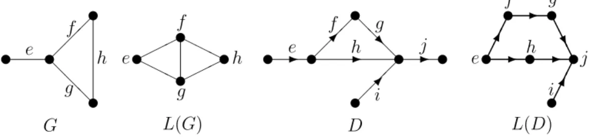
(18) A complete m-partite graph G is an m-partite graph such that the edge uv ∈ E(G) if and only if u and v are in different partite sets. When m ≥ 2, we write Kn1 ,n2 ,...,nm for the complete m-partite graph with partite sets of sizes n1 , n2 , . . . , nm . Moreover, if n1 = n2 = · · · = nm = n, then it is called a balanced complete m-partite graph and denoted Km(n) . A balanced complete multipartite graph is a balanced complete m-partite graph with m ≥ 2. A complete graph is a simple graph whose vertices are pairwise adjacent; the complete graph with m vertices is denoted Km . We can also view a complete graph Km as a balanced complete m-partite graph Km(n) with n = 1. A graph with no cycle is acyclic. A forest is an acyclic graph. A tree is a connected acyclic graph. A leaf is a vertex of degree 1. A spanning subgraph of G is a subgraph with vertex set V (G). A spanning tree is a spanning subgraph that is a tree. A tree is a connected forest, and every component of a forest is a tree. A star is a tree consisting of one vertex adjacent to all the others. The star of order n is the complete bipartite graph K1,n−1 . The line graph of a graph G, written L(G), is the graph whose vertices are the edges of G, with ef ∈ E(L(G)) when e = uv and f = vw in G. Substituting “digraph” for “graph” in this sentence yields the definition of line digraph. For graphs, e and f share a vertex; for digraphs, the head of e must be the tail of f . Figure 1.6 shows a graph G and its line digraph L(G); a digraph D and its line digraph L(D).. u e. u f f¡ u ¡ © HH © © Huh ¡ u h eu HH ©© @ H© u g@ g @u. G. u f ¡@ g ¡ R µ j e u h@ @u - u ¡ u¡ ¡ µ ¡i u. L(G). D. f. g. u- u A ¢ ¸¢ h UA e ¢u - u - Auj ¢ ¢ ¸ iu ¢. L(D). Figure 1.6: G and its line graph L(G); D and its line digraph L(D).. Finally, for x ∈ R, the floor bxc is the greatest integer that is at most x. The ceiling dxe is the smallest integer that is at least x. 8.

(19) 1.4. Switching Networks. The need of a switching network came from the requirements to interconnect pairs of telephones. At first, when there were not so many phones, a direct wire was installed between every two phones. However, with the increase in the number of phones, the transmission cost of these wires became overbearing and the notion of switching was born. Every phone in a given locality was then connected to a “switching” center where the wires from these phones were interconnected through a network called switching networks. Later, it was reinvented for the parallel computer to interconnect processors with memories. Currently, it is intended for many other applications such as data transmission, video rental, conference calls, and broadcast. It is safe to say that the need of switching networks is expanding fast. A switching network can interconnect either one group of users, called a 1-sided network, or two groups, called a 2-sided network. The dominant applications and theory for switching networks are 2-sided. For many applications, the two sides represent two different types of entities; so input x connecting to output y is not the same as input y connecting to output x. Note that a 2-sided network can be used as a 1-sided network by putting the same type of entities on both sides, although this is less economical from the switching viewpoint. In this thesis, we will only deal with 2-sided networks. In the 2-sided case we assume that the network has a set of input terminals and a set of output terminals, while the former generate requests to be connected to the latter through the network. Theoretically, an input terminal can request to be connected to any output terminal, just as one phone can call any other phone. Therefore the network must provide access from any input terminal to every output terminal. Furthermore, once a connection is established, it could last for a period of time, while other input terminals may generate their own requests during this period. What a switching network does is to simultaneously connect these requests, the pattern constantly changing by some terminals hanging up and others making new requests. 9.

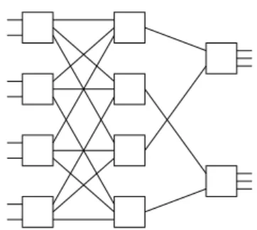
(20) The basic components of a switching network are crossbar switches, or just crossbars, and links which connect crossbars. A crossbar with n inlets and m outlets, denoted Xnm , is said of size n × m. Inlets (outlets) on the same crossbar are called co-inlets (co-outlets). Any one-to-one mapping between the inlets and the outlets of a crossbar is considered routable, i.e., a crossbar is nonblocking. Some crossbars are connected to the outside world. For a 2-sided network, one set of such crossbars will be called input crossbars and the other set output crossbars. The links on an input (output) crossbar linking to the outside world are called inputs (outputs) of the network, and often drawn by open-ended lines. They are also referred to as external links, while other links are internal links. An (N, M )-network has N inputs and M outputs. If M = N , then it is called an N -network. Although a request is originally generated by a pair of input-output, it can be treated as if generated by a pair of input-output crossbars since the crossbar is nonblocking. A request is connected by a path in the network, while two connections do not block each other if their paths are link-disjoint. In an s-stage network, the crossbars are lined up into s columns, each called a stage. Sometimes s is not specified and the network is called a multistage interconnection network (MIN). Crossbars in the same stage have the same size. Links exist only between crossbars in adjacent stages. A link between a crossbar in stage i and a crossbar in stage i + 1 connects an outlet of the former to an inlet of the latter. Crossbars in the first (last) stage are the input (output) crossbars and its inlets (outlets) are the input (output) terminals, sometimes just called inputs (outputs) of the network connected to external lines. The notation for an s-stage network is that stage i has ri crossbars of size ni × mi . Necessarily, ri mi = ri+1 ni+1 for i = 1, 2, . . . , s − 1. Figure 1.7 shows a 3-stage network with 8 inputs and 6 outputs, where r1 = r2 = 4, r3 = 2, n1 = 2, m1 = 3, n2 = 3, m2 = 1, n3 = 2, m3 = 3, and a crossbar is represented by a square. A d-nary network (MIN) is simply a network (a MIN) using only crossbars of size d×d. In a d-nary MIN of size N , a power of d, it is customary to use the notation n = logd N . Note that in a d-nary MIN every stage has the same number of crossbars. 10.

(21) Figure 1.7: A 3-stage MIN.. By treating a crossbar as a vertex and a link as an edge, a switching network is very much like a digraph except that each input (output) crossbar has external links dangling without connecting to any vertex and hence cannot be considered as edges. To remedy this irregularity, the graph theorist prefers to define a true digraph, called a line digraph, from a network by converting each link as a vertex including the inputs and the outputs, while a crosspoint connecting two links in the network becomes an edge in this digraph. Note that a crossbar is represented by a complete bipartite subgraph whose recognizability may depend on the drawing of the line digraph. Figure 1.8 shows the line digraph of the network in Figure 1.7.. Figure 1.8: The line digraph of the network in Figure 1.7.. 11.

(22) 1.5. Overview. The first purpose of this thesis is to determine the linear k-arboricity of a complete multipartite graph. The second purpose of this thesis is to characterize a new network obtained from the line digraph of a bit permutation network. We give an overview of this thesis in the following: In Chapter 1, we list the basic notations, terminologies, and definitions on graph theory and the mathematical theory of switching networks. Chapter 2 is an introduction of the linear k-arboricity problem. This problem has been conjectured that it is NP-complete for any fixed k. However, it is solvable for some classes of graphs, such as cubic graphs, trees, complete graphs, or balanced complete bipartite graphs, and some values of k. Hence, we state the corresponding results which have been determined. In Chapter 3, we consider the linear 3-arboricity problem on balanced complete bipartite graphs, complete graphs, and balanced complete multipartite graphs. We find the linear 3-arboricity of balanced complete bipartite graphs and complete graphs. We also give some substantial results when G is a balanced complete multipartite graph. In Chapter 4, we discuss the linear 2-arboricity problem on complete bipartite graphs, complete graphs, and balanced complete multipartite graphs. We give some substantial results for each class of the graphs above. It is worthy of mentioning that we point out that some computing errors happened in the proof of a result previously [3] and we give a revised result. In Chapter 5, we first introduce the concept of bit permutation networks. Then we list some results about bit permutation networks which are equivalent. Finally, we characterize the network obtained from the line digraph of a bit permutation network. Chapter 6 makes a conclusion, besides stating the results obtained on the linear k-arboricity problem and bit permutation networks, some unsolved questions that we concern most are also mentioned.. 12.

(23) Chapter 2 The Linear k-arboricity Problem A decomposition of a graph is a list of subgraphs such that each edge appears in exactly one subgraph in the list. If a graph G has a decomposition G1 , G2 , . . . , Gd , then we say G can be decomposed into G1 , G2 , . . . , Gd or G1 , G2 , . . . , Gd decompose G. There are many interesting results and problems in this area. A good survey of them is provided by Chung and Graham [8]. In this thesis, we will study a special case of graph decomposition, called the linear k-arboricity problem.. 2.1. Introduction. A linear k-forest is a graph whose components are paths with lengths at most k. The linear k-arboricity of a graph G, denoted lak (G), is the minimum number of linear k-forests needed to decompose G. Then, the linear k-arboricity problem is what the value lak (G) should be when a graph G is given. For example, Figure 2.1 shows that the graph K4 can be decomposed into two linear 3-forests. Thus la3 (K4 ) ≤ 2. In fact, la3 (K4 ) = 2. v. w. v u. u u @ @ u @u. u. w u ¡. ¡ ¡ u u. u. x. x. Figure 2.1: Two linear 3-forests in K4 .. 13.

(24) The notion of linear k-arboricity was defined by Habib and Peroche in [11]. It is a natural generalization of edge coloring. Recall that the chromatic index of a graph G, written χ0 (G), is the least k such that G is k-edge-colorable. Clearly, a linear 1-forest is induced by a matching and la1 (G) = χ0 (G). Linear k-arboricity is also a refinement of the concept of linear arboricity, which is the minimum number of linear forests needed to decompose a graph G and denoted la(G). A linear forest is a graph in which every component is a path with no length constraints. The idea of linear arboricity was introduced earlier by Harary [14]. Next, we describe some properties of lak (G). Lemma 2.1.1. If G is a graph of order n, then la(G) = lan−1 (G) ≤ lan−2 (G) ≤ · · · ≤ la2 (G) ≤ la1 (G) = χ0 (G) ≤ ∆(G) + 1. Lemma 2.1.2. If H is a subgraph of G, then lak (H) ≤ lak (G). Lemma 2.1.3. If a graph G is the edge-disjoint union of two subgraphs G1 and G2 , then lak (G) ≤ lak (G1 ) + lak (G2 ). Lemma 2.1.4. If a graph G is the disjoint union of two graphs G1 and G2 , then lak (G) = max {lak (G1 ), lak (G2 )}. ½l m » ∆(G) , Lemma 2.1.5. lak (G) ≥ max 2. |E(G)| (G)| c b k|Vk+1. ¼¾ .. Lemmas 2.1.1 ∼ 2.1.4 are evident by the definition of linear k-arboricity. In particular, since edges sharing a vertex need different colors, χ0 (G) ≥ ∆(G). Vizing [27] proved that ∆(G) + 1 colors suffice when G is simple. Hence ∆(G) ≤ la1 (G) = χ0 (G) ≤ ∆(G) + 1 in Lemma 2.1.1. We shall use Lemmas 2.1.2 ∼ 2.1.4 frequently without an explicit reference. Since any vertex of a linear k-forest in a graph G has k j k|V (G)| edges, we have degree at most 2 and a linear k-forest in G has at most k+1 Lemma 2.1.5. In the rest of this chapter, we will state some results which have been proved.. 14.

(25) 2.2. The Known Results. In 1981, Holyer [15] obtained the result that determining χ0 (G) (or la1 (G)) of a graph G is NP-complete. Next year, Peroche [22] also proved the NP-completeness of determining la(G). Further, in 1984, Bermond et al. [2] showed that determining whether la3 (G) = 2 is NP-complete for a cubic graph G with |V (G)| ≡ 0 (mod 4) and hence conjectured that it is NP-complete to determine lak (G) for a graph G and any fixed k. Therefore, the linear k-arboricity problem seems to be difficult. In 1982, Habib and Peroche [12] made the following important conjecture: Conjecture 2.2.1. If G is a graph with maximum degree ∆(G) and k ≥ 2, then  » ¼  ∆(G)·|V (G)|  if ∆(G) = |V (G)| − 1 and  (G)|  c  2b k·|Vk+1 lak (G) ≤ ¼ »    ∆(G)·|V (G)|+1  if ∆(G) < |V (G)| − 1.  k·|V (G)| 2b k+1 c e and This conjecture contains Akiyama’s conjecture [1] that la(G) ≤ d ∆(G)+1 2 gives an upper bound about the linear k-arboricity of a graph G. So far, quite a few results on the verification of Conjecture 2.2.1 have been obtained in the literature. For example, when G is a cubic graph, tree, complete graph, or balanced complete e − 1. In what follows, we will bipartite graph, and the value k is small or k ≥ d |V (G)| 2 state them in detail. In 1984, Bermond et al. [2] proved that if G is a graph with maximum degree ∆(G), then lak (G) ≤ ∆(G) for any k ≥ 2. By using this result and Lemma 2.1.5, it is not difficult to know that the linear 2-arboricity of a cubic graph is equal to 3. Moreover, in [2], Bermond et al. also showed that: Theorem 2.2.2. If G is a cubic graph with la3 (G) = 2, then |V (G)| ≡ 0 (mod 4). Hence, for each cubic graph G with |V (G)| ≡ 2 (mod 4), la3 (G) = 3. However, it’s a pity that the determination of la3 (G) is NP-complete for cubic graphs G with |V (G)| ≡ 0 (mod 4). Finally, Bermond et al. conjectured that la5 (G) = 2 if G is a cubic graph. 15.

(26) In 1996, Jackson and Wormald [19] asked a relative question “is it true that la4 (G) = 2 for all cubic graphs G with at least eight vertices?” They also showed that if G is a cubic graph and k ≥ 18, then lak (G) = 2. In 1999, Thomassen [24] proved lak (G) ≤ 2 for a cubic graph G and k ≥ 5. This result is best possible. Next, we study the linear k-arboricity of trees from an algorithmic point of view. Habib and Peroche [11] showed the first result along this line. They gave an algorithm to prove that if T is a tree with exactly one vertex of maximum degree 2θ, then la2 (T ) ≤ θ. Using this as the induction basis, they then gave a characterization for a tree T with maximum degree 2θ to have la2 (T ) = θ. However, Chang [5] pointed out that this characterization has a flaw. He then presented a linear-time algorithm for determining whether a tree T satisfies la2 (T ) ≤ θ and gave a new characterization for a tree T with maximum degree 2θ to have la2 (T ) = θ. As for general k, Chang [5] also proved: Theorem 2.2.3. If T is a tree with ∆(T ) = 2θ − 1 then lak (T ) = θ for k ≥ 2. If T is a tree with ∆(T ) = 2θ then θ ≤ lak (T ) ≤ θ + 1 for k ≥ 2. So, it remains to determine whether lak (T ) is θ or θ + 1 when ∆(T ) = 2θ. Latterly, in [6], Chang et al. gave a linear-time algorithm for answering whether a tree T satisfies lak (T ) ≤ θ for a fixed k. Now, let’s focus on another class of graphs. In 1984, Bermond et al. [2] determined the linear 2-arboricity of complete graphs. They had the following result: ¼ » m(m−1) Theorem 2.2.4. For m 6≡ 10, 11 (mod 12), la2 (Km ) = 2 2m . b3c ¼ » for m ≡ 11 (mod 12), then Bermond et al. also said that if la2 (Km ) = m(m−1) 2b 2m 3 c ¼ » for m ≡ 10 (mod 12). This statement can be proved by Lemmas la2 (Km ) = m(m−1) 2b 2m 3 c ¼ » m(m−1) = 9t + 8. Since 2.1.2 and 2.1.5. Let m = 12t + 11 for any t ≥ 0, then 2 2m b3c K12t+10 ⊆ K12t+11 » , if la2¼(K12t+11 ) = 9t + 8, then la2 (K12t+10 ) ≤ 9t + 8 by Lemma 2.1.2. However,. m(m−1) 2b 2m 3 c. is also equal to 9t + 8 when m = 12t + 10 for any t ≥ 0. 16.

(27) ¼. » Hence, la2 (Km ) ≤. ¼. ». m(m−1) 2b 2m 3 c. for m ≡ 10 (mod 12) if la2 (Km ) =. m ≡ 11 (mod 12). On the other hand, by Lemma 2.1.5, la2 (Km ) ≥. ». m(m−1) 2b 2m 3 c m(m−1) 2b 2m 3 c. for ¼ for. m ≡ 10 (mod 12). In 1991, Chen et al. [3] derived a similar result about the linear 2-arboricity of a complete graph Km by using the ideas from latin squares. They had: m m l l 3(3u+1) and la2 (K3u+2 ) = , la (K ) = Theorem 2.2.5. la2 (K3u ) = 3(3u−1) 2 3u+1 4 4 m l (3u+2)(3u−1) except possibly if 3u + 1 ∈ {49, 52, 58}. 2(2u+1) In [3], Chen et al. indicated the fact that la2 (K12t+11 ) = 9t + 9 for any t ≥ 0. However, some computing errors happened in its proof. In Chapter 4 of this thesis, we will show that la2 (K12t+10 ) and la2 (K12t+11 ) are equal to 9t + 8 for any t 6= 4, which provide the answers of the unsolved cases in Theorem 2.2.4. In 1994, by using similar ideas from latin squares, Fu and Huang [10] also gave the following result about the linear 2-arboricity of a balanced complete bipartite graph Kn,n . 2. Theorem 2.2.6. la2 (Kn,n ) = d b n4n c e. 3. It is worthy of noting that most of the results mentioned above on lak (G) of a graph G have the same property that k is small. Therefore, finally, we state the following results obtained by Chen and Huang [4] on lak (Km ) for k ≥ d m2 e − 1 and on lak (Kn,n ) for k ≥ n − 1. m e − 2. Then Theorem 2.2.7. Suppose m > i ≥ 2 and let d mi e − 1 ≤ k ≤ d i−1. e, and the equality holds in case that i = 2. lak (Km ) ≥ d m(m−1) 2(m−i) 2n e − 2. Then e − 1 ≤ k ≤ d i−1 Theorem 2.2.8. Suppose 2n > i ≥ 2 and let d 2n i 2. n e, and the equality holds in case that i = 2. lak (Kn,n ) ≥ d 2n−i. 17.

(28) Chapter 3 Linear 3-arboricity of Balanced Complete Multipartite Graphs In this chapter, we study the linear 3-arboricity problem on balanced complete bipartite graphs, complete graphs, and balanced complete multipartite graphs. The results obtained are coherent with the corresponding cases of Conjecture 2.2.1.. 3.1. Preliminary Lemmas. Assume that G and H are graphs. A spanning subgraph F of G is called an H-factor if each component of F is isomorphic to H. If G is expressible as an edge-disjoint union of H-factors, then this union is called an H-factorization of G. Furthermore, we say that a 1-factor of a graph G is a spanning 1-regular subgraph of G. A 1-factor and a perfect matching are almost the same thing. The precise distinction is that “1-factor” is a spanning 1-regular subgraph of G, while “perfect matching” is the set of edges in such a subgraph. A decomposition of a regular graph G into 1-factors is a 1-factorization of G. A graph with a 1-factorization is 1-factorable. Let G(X, Y ) be a bipartite graph with bipartition X = {xj | j = 0, 1, . . . , r − 1}, Y = {yj | j = 0, 1, . . . , s − 1}, and |Y | = s ≥ r = |X|. We define the bipartite difference of an edge xp yq in G(X, Y ) as the value q − p (mod s). For example, the bipartite differences of x1 y2 and x3 y0 in a complete bipartite graph K4,7 are 1 and 4. 18.

(29) It is not difficult to see that an edge subset in G(X, Y ) containing the edges of the same bipartite difference must be a matching. In particular, the edge subset is also a perfect matching if G(X, Y ) is a balanced complete bipartite graph Ks,s . Moreover, we can partition the edge set of G(X, Y ) (or Ks,s ) into s edge-disjoint matchings such that each matching is consisting of edges with the same bipartite difference ` ∈ {0, 1, . . . , s − 1} and the edges in different matchings have different bipartite differences. The following lemmas are essential to obtain our results. Lemma 3.1.1. [23] Km has a K3 -factorization if and only if m ≡ 3 (mod 6). Lemma 3.1.2. [13] Km has a K4 -factorization if and only if m ≡ 4 (mod 12). Lemma 3.1.3. A complete graph with even order K2u has a 1-factorization in which there are 2u − 1 1-factors. Proof. We can obtain simply the 1-factors of K2u from a circle and u chords in it. Let the 2u − 1 vertices be placed equally spaced round a circle, and label them 0, 1, . . . , 2u − 2; also label the center 2u − 1. The 1-factor with label i + 1 are then induced by an edge joining vertices i and 2u − 1, and by parallel edges joining the other vertices in pairs. Figure 3.1 shows the case of four vertices. 0. 0. 0. 3. 3. 3. 1. 2. (1). 1. 2. 1. (2). 2. (3). Figure 3.1: A 1-factorization of K4 .. Lemma 3.1.4. If a graph G has an H-factorization with r H-factors, then lak (G) ≤ r · lak (H). 19.

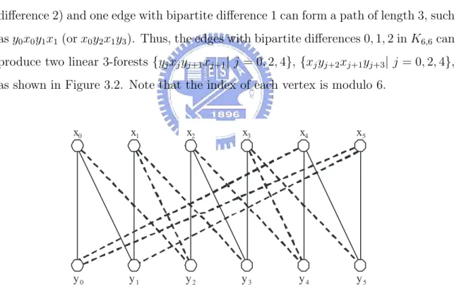
(30) Proof. Since an H-factor of G is a spanning subgraph of G whose components are all isomorphic to H, the linear k-arboricity of every H-factor of G is then equal to lak (H) by Lemma 2.1.4. Since G has an H-factorization with r H-factors, therefore, lak (G) ≤ r · lak (H) by Lemma 2.1.3.. 3.2. Balanced Complete Bipartite Graphs. In this section, we study the linear 3-arboricity of a balanced complete bipartite graph Kn,n . We start with the results of smaller orders. Lemma 3.2.1. la3 (K6,6 ) = 4. Proof. Assume that the vertices of two partite sets in K6,6 are x0 , x1 , . . . , x5 and y0 , y1 , . . . , y5 . Then we observe that two edges with bipartite difference 0 (or bipartite difference 2) and one edge with bipartite difference 1 can form a path of length 3, such as y0 x0 y1 x1 (or x0 y2 x1 y3 ). Thus, the edges with bipartite differences 0, 1, 2 in K6,6 can produce two linear 3-forests {yj xj yj+1 xj+1 | j = 0, 2, 4}, {xj yj+2 xj+1 yj+3 | j = 0, 2, 4}, as shown in Figure 3.2. Note that the index of each vertex is modulo 6.. x0. x1. x2. x3. x4. x5. y0. y1. y2. y3. y4. y5. Figure 3.2: Two linear 3-forests in K6,6 .. Similarly, the edges with bipartite differences 3, 4, 5 in K6,6 also can produce two other linear 3-forests {yj+3 xj yj+4 xj+1 | j = 0, 2, 4}, {xj yj+5 xj+1 yj+6 | j = 0, 2, 4}. 20.

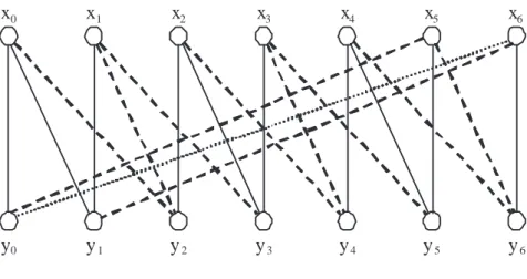
(31) Hence, la3 (K6,6 ) ≤ 4. We construct the array in Figure 3.3 to show this bound. The entry ω in row xγ and column yδ means that the edge xγ yδ appears»in the linear 3-forest ¼ labelled by ω. On the other hand, by Lemma 2.1.5, la3 (K6,6 ) ≥ y0. y1. y2. y3. y4. x0. 1. 1. 2. 3. 3. 4. x1. 4. 1. 2. 2. 3. 4. x2. 3. 4. 1. 1. 2. 3. x3. 3. 4. 4. 1. 2. 2. x4. 2. 3. 3. 4. 1. 1. x5. 2. 2. 3. 4. 4. 1. 36. b 3·12 4 c. = 4.. y5. Figure 3.3: The array shows that la3 (K6,6 ) ≤ 4.. Lemma 3.2.2. la3 (K7,7 ) = 5. Proof. Assume that the vertices of two partite sets in K7,7 are x0 , x1 , . . . , x6 and y0 , y1 , . . . , y6 . Due to the observation mentioned in the proof of Lemma 3.2.1, then the edges with bipartite differences 0, 1, 2 in K7,7 can produce two linear 3-forests {x6 y6 } ∪ {yj xj yj+1 xj+1 | j = 0, 2, 4}, {x6 y1 } ∪ {xj yj+2 xj+1 yj+3 | j = 0, 2, 4} except the edge x6 y0 with bipartite difference 1 which is not being used, as shown in Figure 3.4. We call the edges x6 y6 and x6 y1 base edges because we can construct the whole linear 3-forests from them. Similarly, the edges with bipartite differences 3, 4, 5 in K7,7 also can produce two other linear 3-forests {x5 y1 } ∪ {yj+3 xj yj+4 xj+1 | j = 6, 1, 3}, {x5 y3 } ∪ {xj yj+5 xj+1 yj+6 | j = 6, 1, 3} except the edge x5 y2 with bipartite difference 4 which is not being used. Note that the index of each vertex is modulo 7. Now, let the edges x6 y0 , x5 y2 which are not being used and all edges with bipartite difference 6 in K7,7 form the last linear 3-forest. It is consisting of three isolated edges and two paths of length 3. Thus, la3 (K7,7 ) ≤ 5 and the array 3.5 shows this ¼ » in Figure bound. On the other hand, by Lemma 2.1.5, la3 (K7,7 ) ≥ 21. 49. b 3·14 4 c. = 5..

(32) x0. x1. x2. x3. x4. x5. x6. y0. y1. y2. y3. y4. y5. y6. Figure 3.4: Two linear 3-forests and one isolated edge in K7,7 . y0. y1. y2. y3. y4. y5. x0. 1. 1. 2. 3. 4. 4. 5. x1. 5. 1. 2. 2. 3. 3. 4. x2. 4. 5. 1. 1. 2. 3. 4. x3. 3. 4. 5. 1. 2. 2. 3. x4. 3. 4. 4. 5. 1. 1. 2. x5. 2. 3. 5. 4. 5. 1. 2. x6. 5. 2. 3. 3. 4. 5. 1. y6. Figure 3.5: The array shows that la3 (K7,7 ) ≤ 5.. In what follows, we consider the general cases of n. Proposition 3.2.3. la3 (Kn,n ) = Proof.. 2n 3. if n ≡ 0 (mod 6).. From the proof of Lemma 3.2.1, we observe that if n is even, then the. edges with bipartite differences ², ² + 1, ² + 2 in Kn,n for any ² can produce two linear 3-forests. Hence, the edges with bipartite differences from 0 to n − 1 in Kn,n ¡ ¢ linear 3-forests. On the other hand, by Lemma 2.1.5, · 2 = 2n can generate» n3 ¼ 3 2 if n ≡ 0 (mod 6). = 2n la3 (Kn,n ) ≥ n3n 3 b2c § ¨ if n ≡ 4 (mod 6). Proposition 3.2.4. la3 (Kn,n ) = 2n 3 22.

(33) Proof. First, by using the method in the proof of Proposition 3.2.3, the edges with ¢ ¡ linear · 2 = 2(n−1) bipartite differences from 0 to n − 2 in Kn,n can generate n−1 3 3 3-forests. Next, the edges with bipartite difference n−1 in Kn,n can uniquely produce § ¨ if n ≡ 4 (mod 6). On = 2n + 1»= 2n+1 a linear 3-forest. Thus la3 (Kn,n ) ≤ 2(n−1) 3 3¼ 3 ¨ § 2 if n ≡ 4 (mod 6). = 2n the other hand, by Lemma 2.1.5, la3 (Kn,n ) ≥ n3n 3 b2c § ¨ if n ≡ 2 (mod 6). Proposition 3.2.5. la3 (Kn,n ) = 2n 3 Proof. The edges with bipartite differences from 0 to n − 3 in Kn,n can generate ¡ n−2 ¢ linear 3-forests. The edges with bipartite differences n − 2 and · 2 = 2(n−2) 3 3 n − 1 in Kn,n can produce different linear 3-forests respectively. Thus la3 (Kn,n ) ≤ § ¨ 2(n−2) if n ≡ 2 (mod 6). On the other hand, by Lemma 2.1.5, = 2n + 2 =» 2n+2 3 3 ¼ 3 ¨ § 2 if n ≡ 2 (mod 6). = 2n la3 (Kn,n ) ≥ n3n 3 b2c § ¨ if n ≡ 5 (mod 6). Proposition 3.2.6. la3 (Kn,n ) = 2n 3 Proof. By Proposition 3.2.3, la3 (Kn,n ) ≤ la3 (Kn+1,n+1 ) =. 2(n+1) 3. n ≡ 5 (mod 6). On the other hand, by Lemma 2.1.5, la3 (Kn,n ) ≥. = ». 2n+2 3 ¼. =. n2. =. b 3n2 c. § 2n ¨ 3. if. 3. if. § 2n ¨. n ≡ 5 (mod 6). Proposition 3.2.7. la3 (Kn,n ) =. § 2n+2 ¨ 3. if n ≡ 3 (mod 6).. m l ¨ § . On = 2n+2 Proof. By Proposition 3.2.4, la3 (Kn,n ) ≤ la3 (Kn+1,n+1 ) = 2(n+1) 3 3 ¼ » ¨ § 2 if n ≡ 3 (mod 6). = 2n+2 the other hand, by Lemma 2.1.5, la3 (Kn,n ) ≥ n3n 3 b2c § ¨ if n ≡ 1 (mod 6). Proposition 3.2.8. la3 (Kn,n ) = 2n 3 Proof. Assume that the vertices of two partite sets X, Y in Kn,n are x0 , x1 , . . . , xn−1 and y0 , y1 , . . . , yn−1 . First, from the proof of Lemma 3.2.2, we observe that if n is odd, then the edges with bipartite differences ², ² + 1, ² + 2 in Kn,n for any ² can produce two linear 3-forests except one edge with bipartite difference ² + 1 which is not being used. Thus, the edges with bipartite differences from 0 to n − 2 in Kn,n can generate ¡ n−1 ¢ edges which are not being used. linear 3-forests except n−1 · 2 = 2(n−1) 3 3 3 Next, without loss of generality, suppose that those. 2(n−1) 3. linear 3-forests are. constructed from the base edges in {xn−j yn−j+3(j−1) , xn−j yn−j+3(j−1)+2 | 1 ≤ j ≤ 23. n−1 }, 3.

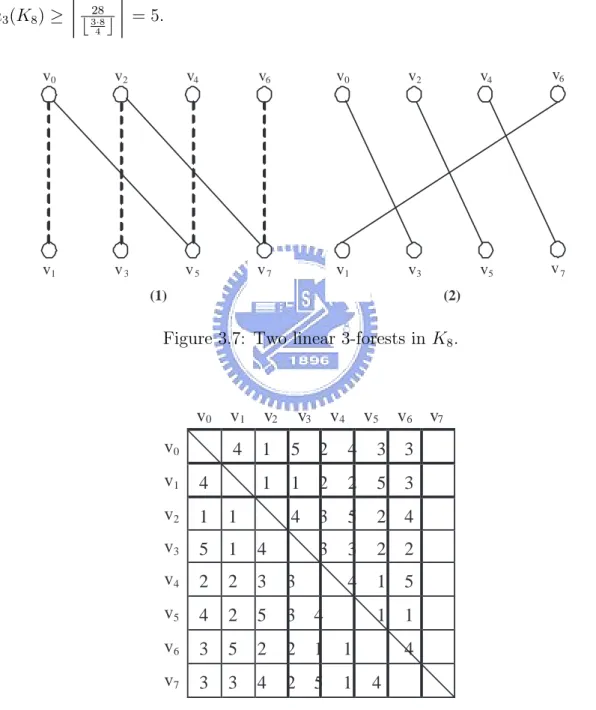
(34) where the index of each vertex is modulo n. Then, the set of those are not being used is a matching {xn−j yn−j+3(j−1)+1 | 1 ≤ j ≤. n−1 3. n−1 }, 3. edges which denoted M1 .. Moreover, the set of edges with bipartite difference n − 1 in Kn,n is a perfect matching {xj yj−1 | 0 ≤ j ≤ n − 1}, denoted M2 . In what follows, we want to show that the edges of M1 and M2 can produce a linear 3-forest together. Since the endpoints u, v of an edge in M1 are incident to two other edges e1 , e2 in M2 , it suffices to prove that the endpoints of e1 , e2 except u, v are not the endpoints of edges in M1 . Since the endpoints in partite set X of edges in M1 are xn−1 , xn−2 , . . . , x 2(n−1) +1 , 3. they are adjacent to the endpoints yn−2 , yn−3 , . . . , y 2(n−1) of edges in M2 . Similarly, the 3. endpoints in partite set Y of edges in M1 are y0 , y2 , . . . , y 2(n−1) −2 , which are adjacent to 3. the endpoints x1 , x3 , . . . , x 2(n−1) −1 of edges in M2 . Note that the endpoints mentioned 3. above are distinct. Hence, each component of the subgraph induced by M1 ∪ M2 is a path of length at most 3 and then we have a linear 3-forest in Kn,n . § ¨ if n ≡ 1 (mod 6). On the other = 2n + 1» = 2n+1 Therefore, la3 (Kn,n ) ≤ 2(n−1) 3 3¼ 3 § ¨ 2 if n ≡ 1 (mod 6). = 2n hand, by Lemma 2.1.5, la3 (Kn,n ) ≥ n3n 3 b2c From the propositions given above, we determine the linear 3-arboricity of Kn,n for any n and conclude the work of this section with the following theorem.. Theorem 3.2.9. & la3 (Kn,n ) =. 2. n ¥ 3n ¦ 2. 3.3. ' =.  § 2n ¨  3. if n ≡ 0, 1, 2, 4, 5 (mod 6),.  § 2n+2 ¨. if n ≡ 3 (mod 6).. 3. Complete Graphs. In this section, we study the linear 3-arboricity of a complete graph Km and the results on Kn.n will give us great help. We start with the case m = 8 of Km . Lemma 3.3.1. la3 (K8 ) = 5. 24.

(35) Proof.. Assume that the vertices of K8 are v0 , v1 , . . . , v7 . First, let the perfect. matching {v2i v2i+1 | 0 ≤ i ≤ 3} of K8 be denoted M . Then, for 0 ≤ i ≤ 3, we define Ni as the set of one edge v2i v2i+1 and its endpoints v2i , v2i+1 . Thus K8 can be viewed as K4 with nodes Ni for 0 ≤ i ≤ 3 and unordered pairs of nodes (Nα , Nβ ) for 0 ≤ α 6= β ≤ 3. The notation (Nα , Nβ ) also means the 4-cycle consisting of the edges v2α v2β , v2α v2β+1 , v2α+1 v2β , and v2α+1 v2β+1 in original K8 . From the proof of Lemma 3.1.3, we know that K4 has a 1-factorization, in which there are three different 1-factors and each 1-factor owns two disjoint unordered pairs of nodes. For example, the 1-factor with label 1 has unordered pairs of nodes (N0 , N3 ) and (N1 , N2 ). Then, from this 1-factor, we observe that the subgraph consisting of two paths v6 v0 v7 v1 in (N0 , N3 ) and v2 v4 v3 v5 in (N1 , N2 ) is a linear 3-forest in original K8 , labelled by 1. However, each of (N0 , N3 ) and (N1 , N2 ) has an edge which is not being used to construct the linear 3-forest with label 1, they are v6 v1 and v2 v5 . Figure 3.6 shows the linear 3-forest with label 1 in original K8 . Similarly, the other 1-factors of K4 can produce two other linear 3-forests in original K8 , labelled by 2 and 3, except the edges v2 v7 , v0 v5 , v4 v7 , and v0 v3 not being used.. N0. N3. v0. v1. v2. v3. N1. v6. v7. v4. v5. N2. Figure 3.6: A linear 3-forest in K8 .. Now, let G(X, Y ) be a bipartite graph with bipartition X = {v0 (= x0 ), v2 (= x1 ), v4 (= x2 ), v6 (= x3 )} and Y = {v1 (= y0 ), v3 (= y1 ), v5 (= y2 ), v7 (= y3 )}. Then those edges which are not being used are exactly all of edges with bipartite difference 1 in G(X, Y ) and half of edges with bipartite difference 2 in G(X, Y ). 25.

(36) We observe that the edges which are half of edges with bipartite difference 2 in G(X, Y ) and all edges of M can produce a linear 3-forest labelled by 4 in original K8 , as shown in Figure 3.7(1). Moreover, the edges with bipartite difference 1 in G(X, Y ) also can produce a linear 3-forest labelled by 5 in original K8 because they form a perfect matching, as shown in Figure 3.7(2). Therefore, la3 (K8 ) ≤ 5. We construct the array in ¼ 3.8 to show this bound. On the other hand, by Lemma 2.1.5, » Figure 28 = 5. la3 (K8 ) ≥ b 3·8 4 c v0. v2. v4. v6. v0. v2. v4. v6. v1. v3. v5. v7. v1. v3. v5. v7. (1). (2). Figure 3.7: Two linear 3-forests in K8 .. v0 v0. v1. v2. v3. v4. v5. 4. 1. 5 2. 4. 3 3. 1. 1 2. 2. 5 3. 4 3. 5. 2 4. 3. 3. 2 2. 4. 1 5. v1. 4. v2. 1. 1. v3. 5. 1. 4. v4. 2. 2. 3. 3. v5. 4. 2. 5. 3 4. v6. 3. 5. 2. 2 1. 1. v7. 3. 3. 4. 2 5. 1. v6 v7. 1 1 4 4. Figure 3.8: The array shows that la3 (K8 ) ≤ 5.. 26.

(37) Lemma 3.3.2. la3 (K10 ) = 7. Proof. Assume that the vertices of K10 are v0 , v1 , . . . , v9 . First, let the matching {v2i v2i+1 | 0 ≤ i ≤ 3} of K10 be denoted M . Then, for 0 ≤ i ≤ 3, we define Ni as the set {v2i , v2i+1 , v2i v2i+1 }. Thus K10 can be viewed as K6 with nodes v8 , v9 , Ni for 0 ≤ i ≤ 3 and unordered pairs of nodes (v8 , Nα ), (v9 , Nβ ), (Nα , Nβ ) for 0 ≤ α 6= β ≤ 3. From the proof of Lemma 3.1.3 (by placing v8 , N0 , . . . , N3 equally spaced round a circle and v9 the center), K6 has a 1-factorization in which there are five different 1-factors and each 1-factor owns three disjoint unordered pairs of nodes. For example, the 1-factor with label 1 has (v8 , v9 ), (N0 , N3 ), and (N1 , N2 ). From this 1-factor, we can then construct a linear 3-forest labelled by 1 in original K10 , as shown in Figure 3.9. However, the edges v6 v1 in (N0 , N3 ) and v2 v5 in (N1 , N2 ) are not being used.. N0. v0. v1. v8. v2. v3. N1. N3. v6. v7. v9. v4. v5. N2. Figure 3.9: A linear 3-forest in K10 .. Similarly, the other 1-factors of K6 can produce four other linear 3-forests labelled by 2, 3, 4, 5 in original K10 except the edges v4 v7 , v0 v5 , v2 v7 , and v0 v3 not being used. Figure 3.10 shows the linear 3-forest with label 2 in original K10 . Finally, from the proof of Lemma 3.3.1, the six edges above which are not being used and all edges of M can produce two other linear 3-forests labelled by 6 and 7 in original ¼K10 . Hence, la3 (K10 ) ≤ 7. On the other hand, by Lemma 2.1.5, la3 (K10 ) ≥ » 45 = 7. b 3·10 4 c In what follows, we consider the general cases of m. 27.

(38) N0. N1. v0. v1. v8. v4. v5. N2. v2. v3. v9. v6. v7. N3. Figure 3.10: Another linear 3-forest in K10 .. Proposition 3.3.3. la3 (Km ) =. § 2m−2 ¨ 3. if m ≡ 0, 4, 8 (mod 12).. Proof. Assume that the vertices of Km are v0 , v1 , . . . , vm−1 . First, let the perfect ª © matching v2i v2i+1 | 0 ≤ i ≤ m2 − 1 of Km be denoted M . Then, for 0 ≤ i ≤ m2 − 1, we define Ni as the set {v2i , v2i+1 , v2i v2i+1 }. Thus Km can be viewed as K m2 with nodes Ni for 0 ≤ i ≤. m 2. − 1 and unordered pairs of nodes (Nα , Nβ ) for 0 ≤ α 6= β ≤. From the proof of Lemma 3.1.3, K m2 can be decomposed into 1-factors and each 1-factor owns. m 4. m 2. m 2. − 1.. − 1 different. disjoint unordered pairs of nodes. Since each. unordered pair of nodes in K m2 is composed of a path with length 3 and one edge in original Km , then a 1-factor of K m2 can produce one linear 3-forest in original Km m 2. except. m 4. edges which are not being used. Hence, from the. obtain. m 2. − 1 linear 3-forests in original Km except ( m2 − 1) · m4 edges not being used.. − 1 1-factors of K m2 , we. Now, let G(X, Y ) be a bipartite graph with bipartition X = {v2i (= xi )| 0 ≤ i ≤ m 2. − 1} and Y = {v2i+1 (= yi )| 0 ≤ i ≤. m 2. − 1}. Then those edges which are not being. used are exactly all of edges with bipartite differences 1, 2, . . . , m4 − 1 in G(X, Y ) and half of edges with bipartite difference. m 4. in G(X, Y ).. We observe that the edges which are half of edges with bipartite difference. m 4. in. G(X, Y ) and all edges of M can produce a linear 3-forest in original Km . Moreover, since the size of X (or Y ) is even and |X| = |Y |, the edges with bipartite differences ², ² + 1, ² + 2 in G(X, Y ) for any ² can produce two linear 3-forests from the proof of Proposition 3.2.3. Thus, the edges with bipartite differences 1, 2, . . . , m4 − 1 in m § l m ¨ −1 other linear 3-forests in original Km . G(X, Y ) can generate ( 4 3 ) · 2 = m−4 6 28.

(39) ¨ § 2m−2 ¨ § . On the other hand, by = Therefore, la3 (Km ) ≤»( m2 − 1)¼+ 1 + m−4 3 6 ¨ § if m ≡ 0, 4, 8 (mod 12). = 2m−2 Lemma 2.1.5, la3 (Km ) ≥ m·(m−1) 3 2·b 3m 4 c § ¨ if m ≡ 2, 6, 10 (mod 12). Proposition 3.3.4. la3 (Km ) = 2m 3 Proof. Assume that the vertices of Km are v0 , v1 , . . . , vm−1 . First, let the matching ª © − 1, we − 1 of Km be denoted M . Then, for 0 ≤ i ≤ m−2 v2i v2i+1 | 0 ≤ i ≤ m−2 2 2 define Ni as the set {v2i , v2i+1 , v2i v2i+1 }. Thus Km can be viewed as K m+2 with 2. nodes vm−2 , vm−1 , Ni for 0 ≤ i ≤. m−2 2. (vm−1 , Nβ ), (Nα , Nβ ) for 0 ≤ α 6= β ≤. − 1 and unordered pairs of nodes (vm−2 , Nα ), m−2 2. Since m ≡ 2, 6, 10 (mod 12), then. − 1.. m+2 2. ≡ 0, 2, 4 (mod 6). From the proof of. Lemma 3.1.3 (by placing vm−2 , N0 , N1 , . . . , N m−2 −1 equally spaced round a circle and 2. vm−1 the center), K. m+2 2. has a 1-factorization in which there are. 1-factors and each 1-factor owns. m+2 4. m+2 2. − 1 different. disjoint unordered pairs of nodes. However,. an unordered pair of nodes (Nα , Nβ ) in K m+2 is composed of a path with length 3 2. and one edge in original Km . Hence, each 1-factor of K m+2 can produce one linear 2. 3-forest in original Km and leaves. m+2 4. − 2 edges which are not being used except the. 1-factor with label 1 which contains the unordered pair of nodes (vm−2 , vm−1 ) leaves m+2 4. − 1 edges not being used. Therefore, from the. obtain. m+2 2. − 1 linear 3-forests in original Km except. m+2 2. − 1 1-factors of K m+2 , we. ( m+2 2. 2. −. 1) · ( m+2 4. − 2) + 1 edges. not being used. Now, let G(X, Y ) be a bipartite graph with bipartition X = {v2i (= xi )| 0 ≤ i ≤ m−2 2. − 1} and Y = {v2i+1 (= yi )| 0 ≤ i ≤. m−2 2. − 1}. Then those edges which are. − 1 in not being used are exactly all of edges with bipartite differences 1, 2, . . . , m−2 4 G(X, Y ) and half of edges with bipartite difference. m−2 4. in G(X, Y ).. We observe that the edges which are half of edges with bipartite difference. m−2 4. in. G(X, Y ) and all edges of M can produce a linear 3-forest in original Km . Moreover, since the size of X (or Y ) is even and |X| = |Y |, the edges with bipartite differences ², ² + 1, ² + 2 in G(X, Y ) for any ² can produce two linear 3-forests from the proof − 1 in of Proposition 3.2.3. Thus, the edges with bipartite differences 1, 2, . . . , m−2 4 m § l m−2 ¨ −1 other linear 3-forests in original Km . G(X, Y ) can generate ( 4 3 ) · 2 = m−6 6 29.

(40) § 2m ¨ § m−6 ¨ . On the other hand, by = − 1) + 1 + Therefore, la3 (Km ) ≤»( m+2 3 6 2 ¼ ¨ § if m ≡ 2, 6, 10 (mod 12). = 2m Lemma 2.1.5, la3 (Km ) ≥ m·(m−1) 3 2·b 3m 4 c § ¨ if m ≡ 1, 9 (mod 12). Proposition 3.3.5. la3 (Km ) = 2m 3 Proof. Assume that the vertices of Km are v0 , v1 , . . . , vm−1 . First, let the matching ª © − 1, − 1 of Km be denoted M . Then, for 0 ≤ i ≤ m−1 v2i v2i+1 | 0 ≤ i ≤ m−1 2 2 we define Ni as the set {v2i , v2i+1 , v2i v2i+1 }. Thus Km can be viewed as the union of K1, m−1 and K m−1 . The star K1, m−1 has nodes vm−1 , Ni for 0 ≤ i ≤ 2. 2. 2. and unordered pairs of nodes (vm−1 , Ni ) for 0 ≤ i ≤ K m−1 has nodes Ni for 0 ≤ i ≤ 2. 0 ≤ α 6= β ≤ Since. m−1 2. m−1 2. m−1 2. m−1 2. m−1 2. −1. − 1; the complete graph. − 1 and unordered pairs of nodes (Nα , Nβ ) for. − 1.. is even, from the proof of Lemma 3.1.3 (by placing N0 , N1 , . . . , N m−1 −2 2. equally spaced round a circle and N m−1 −1 the center), K m−1 has a 1-factorization 2. 2. in which there are. m−1 2. − 1 different 1-factors and each 1-factor owns. m−1 4. disjoint. unordered pairs of nodes. It is worthy of mentioning that each 1-factor of K m−1 2. has at most one unordered pair of nodes (Ni , Ni+1 ) for some i ∈ {0, 1, . . . ,. m−1 2. − 3}.. Moreover, an unordered pair of nodes (Ni , Ni+1 ) in K m−1 is composed of a path 2. v2i v2i+2 v2i+1 v2i+3 and one edge v2i v2i+3 in original Km . Hence, as the proof of the propositions previously, each 1-factor of K m−1 can 2. produce one linear 3-forest in original Km except used. So, from the. m−1 2. m−1 4. − 1 1-factors of K m−1 , we obtain 2. edges which are not being m−1 2. − 1 linear 3-forests in. ) edges not being used. − 1) · ( m−1 original Km except ( m−1 4 2 Next, for each linear 3-forest obtained from a 1-factor has (Ni , Ni+1 ) for some − 3}, we replace the path v2i v2i+2 v2i+1 v2i+3 in (Ni , Ni+1 ) by another i ∈ {0, 1, . . . , m−1 2 path v2i+3 v2i vm−1 v2i+1 in (Ni , Ni+1 ) and (vm−1 , Ni ). For example, consider the linear 3-forest in K13 obtained from the 1-factor has (N0 , N1 ), we replace the path v0 v2 v1 v3 in (N0 , N1 ) by v3 v0 v12 v1 in (N0 , N1 ) and (v12 , N0 ), as shown in Figure 3.11. −4 Then, let the replaced paths v2i v2i+2 v2i+1 v2i+3 in (Ni , Ni+1 ) for i = 0, 2, . . . , m−1 2 and another path vm−2 vm−5 vm−1 vm−4 in (N m−1 −2 , N m−1 −1 ) and (vm−1 , N m−1 −2 ) form 2. a linear 3-forest in original Km . 30. 2. 2.

(41) N3 v6. N2 v7. v4. N0 v5. v1. v0. v12 v10. v11. v8. v9. v3. v2. N5. N4. N1. N3. N2. N0. v6. v7. v4. v5. v1. v0. v12 v10. v11 N5. v8. v9. v3. v2. N4. N1. Figure 3.11: The process of replacing the paths of length 3.. −3 Also let the replaced paths v2i v2i+2 v2i+1 v2i+3 in (Ni , Ni+1 ) for i = 1, 3, . . . , m−1 2 and another path v1 vm−3 vm−1 vm−2 in (N m−1 −1 , N0 ) and (vm−1 , N m−1 −1 ) form a linear 2. 2. 3-forest in original Km . Thus, the edges appear in K. 1, m−1 2. (N m−1 −1 , N0 ), (Ni , Ni+1 ) for 0 ≤ i ≤ 2. m−1 2. and the edges appear in. − 2 of K m−1 are all being used. 2. Now, let G(X, Y ) be a bipartite graph with bipartition X = {v2i (= xi )| 0 ≤ i ≤ m−1 2. − 1} and Y = {v2i+1 (= yi )| 0 ≤ i ≤. m−1 2. − 1}. Then those edges which are. − 1 in not being used are exactly all of edges with bipartite differences 2, 3, . . . , m−1 4 G(X, Y ) and half of edges with bipartite difference. m−1 4. in G(X, Y ).. We observe that the edges which are half of edges with bipartite difference. m−1 4. in. G(X, Y ) and all edges of M can produce a linear 3-forest in original Km . Moreover,. 31.

(42) since the size of X (or Y ) is even and |X| = |Y |, from the proof of Proposition 3.2.3, the edges with bipartite differences ², ² + 1, ² + 2 in G(X, Y ) for any ² can produce − 1 in two linear 3-forests. Hence, the edges with bipartite differences 2, 3, . . . , m−1 4 m § l m−1 ¨ −2 other linear 3-forests in original Km . G(X, Y ) can generate ( 4 3 ) · 2 = m−9 6 § m−9 ¨ § 2m ¨ = 3 . On the other hand, by − 1) + 2 + 1 + Therefore, la3 (Km ) ≤ »( m−1 6 2 ¼ ¨ § if m ≡ 1, 9 (mod 12). = 2m Lemma 2.1.5, la3 (Km ) ≥ m·(m−1) 3 2·b 3m 4 c § ¨ if m ≡ 3, 7 (mod 12). Proposition 3.3.6. la3 (Km ) = 2m 3 m § ¨ l . On the = 2m Proof. By Proposition 3.3.3, la3 (Km ) ≤ la3 (Km+1 ) = 2(m+1)−2 3 3 ¼ » § 2m ¨ if m ≡ 3, 7 (mod 12). = other hand, by Lemma 2.1.5, la3 (Km ) ≥ m(m−1) 3m 3 2b 4 c § ¨ if m ≡ 5 (mod 12). Proposition 3.3.7. la3 (Km ) = 2m 3 l Proof. By Proposition 3.3.4, la3 (Km ) ≤ la3 (Km+1 ) =. 2(m+1) 3. m =. § 2m+2 ¨ ». 3. = ¼. m(m−1) 2b 3m 4 c. m ≡ 5 (mod 12). On the other hand, by Lemma 2.1.5, la3 (Km ) ≥. § 2m ¨. if § 2m ¨. 3. =. 3. if m ≡ 5 (mod 12). Proposition 3.3.8. la3 (Km ) =. § 2m−2 ¨ 3. if m ≡ 11 (mod 12).. Proof. Assume that the vertices of Km are v0 , v1 , . . . , vm−1 . First, let the matching ª © − 1, we − 1 of Km be denoted M . Then, for 0 ≤ i ≤ m−1 v2i v2i+1 | 0 ≤ i ≤ m−1 2 2 define Ni as the set {v2i , v2i+1 , v2i v2i+1 }. Thus Km can be viewed as K m+1 with nodes 2. vm−1 , Ni for 0 ≤ i ≤ 0 ≤ α 6= β ≤ Since. m+1 2. m−1 2. m−1 2. − 1 and unordered pairs of nodes (vm−1 , Nα ), (Nα , Nβ ) for. − 1.. is even, from the proof of Lemma 3.1.3 (by placing N0 , N1 , . . . , N m−1 −1 2. equally spaced round a circle and vm−1 the center), K m+1 has a 1-factorization in 2. which there are. m+1 2. − 1 different 1-factors and each 1-factor owns. m+1 4. disjoint un-. ordered pairs of nodes. It is worthy of mentioning that each 1-factor of K m+1 contains 2. exactly one unordered pair of nodes (vm−1 , Ni ) for some i ∈ {0, ...,. m−1 2. − 1}.. Hence, as the proof of the propositions previously, a 1-factor of K m+1 can produce 2. one linear 3-forest in original Km except. m+1 4. 32. − 1 edges which are not being used. So,.

(43) from the. m+1 2. − 1 1-factors of K m+1 , we obtain 2. m+1 2. − 1 linear 3-forests in original Km. − 1) edges not being used. − 1) · ( m+1 except ( m+1 4 2 Now, let G(X, Y ) be a bipartite graph with bipartition X = {v2i (= xi )| 0 ≤ i ≤ m−1 2. − 1} and Y = {v2i+1 (= yi )| 0 ≤ i ≤. m−1 2. − 1}. Then those edges which are. not being used and the edges of M are exactly all of edges with bipartite differences c in G(X, Y ). Since the size of X (or Y ) is odd and |X| = |Y |, from 0, 1, . . . , b m−1 4 the proof of Proposition 3.2.8, the edges with bipartite differences ², ² + 1, ² + 2 in G(X, Y ) for any ² can produce two linear 3-forests except one edge with bipartite difference ² + 1 which is not being used. Thus, the edges with bipartite differences m § l m−1 ¨ b 4 c+1 other linear 3-forests ) · 2 = m+1 c in G(X, Y ) can generate ( 0, 1, . . . , b m−1 6 3 4 § m+1 ¨ § m+1 ¨ labelled by 1, 2, . . . , 6 except 12 edges which are still not being used. For example, let’s consider Km with m = 23. Then the partite sets of G(X, Y ) are X = {v0 , v2 , . . . , v20 } and Y = {v1 , v3 , . . . , v21 }. Moreover, the edges with bipartite differences 0, 1, . . . , 5 in G(X, Y ) can produce four linear 3-forests labelled by 1, 2, 3, 4 except two edges v18 v5 , v20 v1 with bipartite differences 4 and 1 respectively which are still not being used, as shown in Figure 3.12. v1. v3. 1. 1. 2. 3. 4 4. 1. 2. 2. 3 3. 4. 1. 1. 2 3. 4 4. 1. 2 2. 3 3. 4. v8. 1 1. 2 3. 4. 4. v 10. 1. 2 2. 3. 3. 4. 1 1. 2. 3. 4. 1. 2. 2. 3. 1. 1. 2. 1. 2. v0 v2. v5 v 7 v 9 v11 v13 v15 v17 v19 v21. v4 v6. v 12 4 v 14 3. 4. v 16 3. 4. v 18 2. 3. v 20. 2. 4 4 3. 3. 1. 4. Figure 3.12: The array shows four linear 3-forests in G(X, Y ).. 33.

(44) Next, we plan to put the. § m+1 ¨ 12. edges which are still not being used into the. linear 3-forest with label 1 and interchange its edges with the edges of another linear 3-forests such that no more linear 3-forests needed to decompose Km . The linear 3−3 forest with label 1 is consisting of the paths v2i+1 v2i v2i+3 v2i+2 for all i = 0, 2, ..., m−1 2 and the base edge vm−3 vm−2 . We start by putting the first edge vm−3 v1 which is still not being used into the linear 3-forest with label 1, then it produce a path P = vm−2 vm−3 v1 v0 v3 v2 , which can not be a component of a linear 3-forest. So, we interchange the edge vm−3 vm−2 in P with another edge vm−2 vm−1 in the linear 3-forest constructed from the 1-factor contains (vm−1 , N m−1 −1 ). Again, we interchange the edge v2 v3 in P with another edge 2. v3 vm−1 in the linear 3-forest constructed from the 1-factor contains (vm−1 , N1 ) and move the edge v3 vm−1 into the linear 3-forest with label 2. Since the linear 3-forest with label 2 is consisting of the paths v2i v2i+5 v2i+2 v2i+7 − 3 and the base edge vm−3 v3 , that movement creates a path for all i = 0, 2, ..., m−1 2 vm−3 v3 vm−1 and we have a new linear 3-forest with label 2. Moreover, the steps above let the length of P become 3. Hence, we also have a new linear 3-forest with label 1, which is consisting of paths with length 3 and one edge vm−2 vm−1 . Note that the index of each vertex is modulo m. Without loss of generality, for 2 ≤ ` ≤. § m+1 ¨ , we assume that the `th edge 12. still not being used is vm−5−4(`−2) v5+2(`−2) , abbreviated to vm−4`+3 v2`+1 . Then, for ¨ § , we put the `th edge vm−4`+3 v2`+1 still not being used sequentially 2 ≤ ` ≤ m+1 12 into the linear 3-forest with label 1 according to the following rules. If ` is even, then we interchange the edge vm−4`+3 vm−4`+4 in the linear 3-forest with label 1 with another edge vm−4`+3 vm−1 in the linear 3-forest constructed from the 1-factor contains (vm−1 , N m−4`+3 ) and move the edge vm−4`+3 vm−1 into the linear 2. 3-forest with label 2`−1. We also interchange the edge v2`+2 v2`+3 in the linear 3-forest with label 1 with another edge v2`+3 vm−1 in the linear 3-forest constructed from the 1-factor contains (vm−1 , N 2`+2 ) and move the edge v2`+3 vm−1 into the linear 3-forest 2. with label 2`. 34.