基於遍佈式電表之智慧型電力排程系統

國

立

交

通

大

學

資訊學院 資訊學程

碩

士

論

文

基於遍佈式電表之智慧型電力排程系統

iPM: An Intelligent Power Scheduling System

Based on Pervasive Meters

研 究 生：廖家良

指導教授：曾煜棋 教授

基於遍佈式電表之智慧型電力排程系統

iPM: An Intelligent Power Scheduling System

Based on Pervasive Meters

研 究 生：廖家良 Student：Jia-Liang Liao

指導教授：曾煜棋 Advisor：Yu-Chee Tseng

國 立 交 通 大 學

資訊學院 資訊學程

碩 士 論 文

Submitted to College of Computer Science National Chiao Tung University in partial Fulfillment of the Requirements

for the Degree of Master of Science

in

Computer Science June 2011

Hsinchu, Taiwan, Republic of China

基 於 遍 佈 式 電 表 之 智 慧 型 電 力 排 程 系 統

學生：

國立交通大學 資訊學院 資訊學程 碩士班

摘

要

iPM: An Intelligent Power Scheduling System

Based on Pervasive Meters

student：

Degree Program of Computer Science

National Chiao Tung University

ABSTRACT

Discovery of electricity is an important mile stone of human

history. It not only contributes to other investigate and also

enriches our life. We can’t live without electricity in our daily life.

However, we found that electric companies usually exceed their

limit of electric output in summer. Therefore, how to use electricity

efficiently is an important subject. For users, what they concern the

most is how to use electricity effectively to save electric cost. In

fact, the cost of electricity varies in different time. The cost of

electric in peak time is higher than Non-peak Time. In this work,

we have proposed a system (iPM) which could schedule electric

appliance which is not urgent to other time which has lower

electric cost. It can not only saves the electric cost for users and

also differentiates the loading of electricity company in peak time

to get a win-win solution.

誌

謝

iPM: An Intelligent Power Scheduling System

Based on Pervasive Meters

Student: Jia-Liang Liao

Advisor: Prof. Yu-Chee Tseng

Department of Computer Science

National Chiao-Tung University

Contents

1 Introduction 1

2 Related Works 4

2.1 ZigBee and Smart Energy Profile . . . 5

3 Design of An Intelligent Power Scheduling System 6

3.1 System Model . . . 6 3.2 Power Scheduling Algorithm . . . 8

4 Prototyping Results 13 4.1 Hardware Components . . . 13 4.2 Software Components . . . 17 5 Simulation Results 18 6 Conclusions 23 Bibliography 24

List of Figures

1.1 Worldwide electricity consumption from World Bank. . . 2

1.2 The system architecture of iPM system. . . 3

3.1 An example of electric appliance types. (a), (b), and (c) are three appliances before scheduling. (d), (e), and (f) are three appliances after scheduling. . . 7

3.2 The flow chart of iPM system. . . 8

3.3 The flow chart of iPM scheduling algorithm. . . 8

3.4 An example of the reference points. . . 9

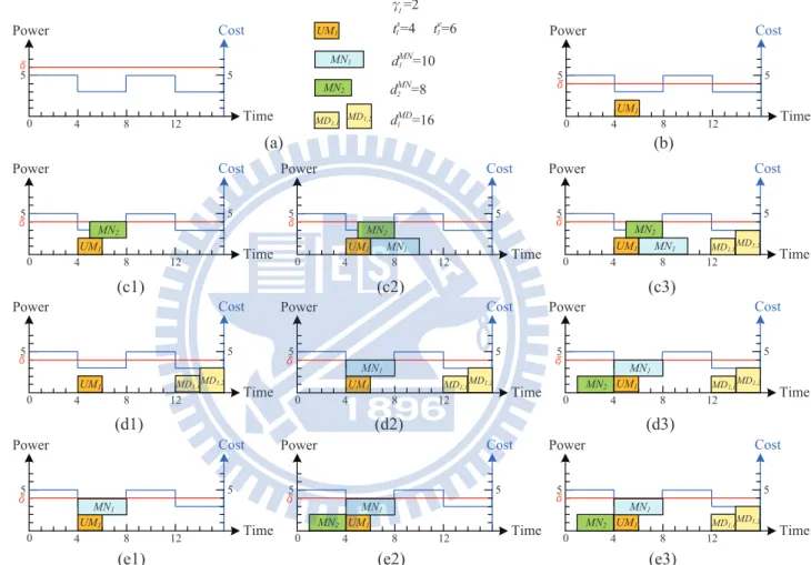
3.5 An example of power scheduling algorithm. (a) The parameters of the example. (b) Scheduling result after insertUC and UM types. (c) Scheduling results by deadline heuristic. (d) Scheduling results by area heuristic. (e) Scheduling results by weight heuristic. . . 12

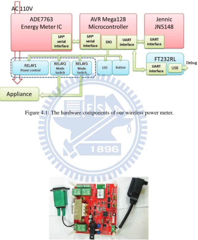
4.1 The hardware components of our wireless power meter. . . 14

4.2 Our implemented wireless power meter. . . 14

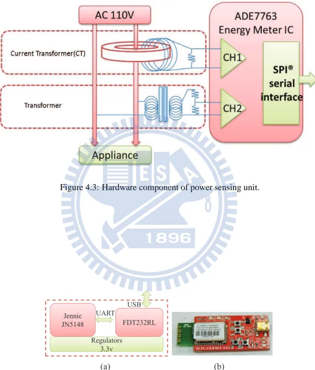
4.3 Hardware component of power sensing unit. . . 15

4.4 The hardware component of iPM system. (a) The hardware components of our sink receiver. (b) Our implemented sink receiver. . . 15

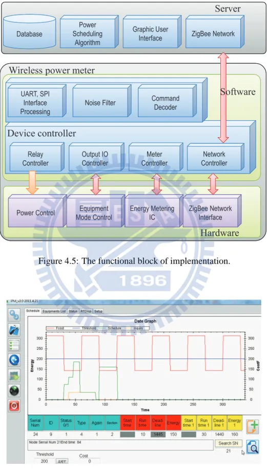
4.5 The functional block of implementation. . . 16

4.6 The graphic user interface of control server. . . 16

5.1 The fluactuating prices during the simulation time. . . 19

5.2 The accumulative power of (a) Deadline heuristic, (b) Area heuristic, (c) Weight heuristic, and (d) incorporation. . . 20

5.3 The power of (a) Deadline heuristic, (b) Area heuristic, (c) Weight heuristic, and (d) incorporation during the simulation time. . . 21

Chapter 1

Introduction

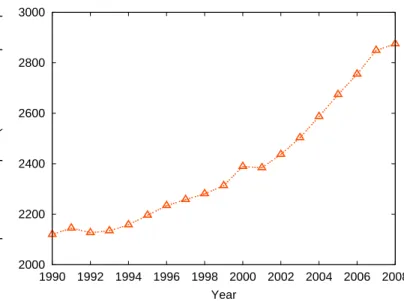
As the standard of living and technological advancements, the electricity consumption of people increases year by year, as shown in Fig. 1.1 [5]. The growing consumption of electricity has put pressure on the power plants to operate at their capacity limit, and thus the consumers would get an expensive electricity bill. In order to prune electricity consumption and lower electricity bill, the smart grid was proposed. The smart grid provides intelligent features for electricity producers and consumers to communicate with one another so as to adjust electricity load. Therefore, one important benefit of a smart grid application is time-based pricing because customers can set their threshold and adjust their usage to take advantage of fluctuating prices. This would depend on the energy management mechanism to control electric appliances and equipment and thus customers could reduce their electricity consumption and save money.

The ZigBee Smart Energy Profile provides the smart grid mechanism for companies and home owners to create a more energy efficient home environment. ZigBee-enabled meters deployed in a home are used to communicate and control ZigBee enabled devices, such as the heating, cooling and air conditioning systems, to enable energy utility programs, including demand response, load control, time of use pricing, etc.. These programs not only reduce the peak load on the utility grid, but help the home users make smart decisions about their energy usage.

In this paper, we propose an intelligent power scheduling system (iPM) based on pervasive meters. Fig. 1.2 shows our system architecture. Each electric appliance connects to a wireless power meter. Through these wireless meters, the current power consumption of electric appli-ances can be transmitted to the control server. In accordance with the execution characteristics of electric appliances, they can be classified into four types: UC (uncontrollable) type, UM (un-movable) type, MN (movable and non-divisible) type, and MD (movable and divisible) type. Our goal is to dynamically schedule the execution time of each electric appliance in a home to

2000 2200 2400 2600 2800 3000 2008 2006 2004 2002 2000 1998 1996 1994 1992 1990

Electric power consumption (kilowatt-hours per capita)

Year

Figure 1.1: Worldwide electricity consumption from World Bank.

minimize the total monetary cost. Still, it poses several challenges: 1) user demand response, 2) load management, and 3) minimizing the monetary cost of electricity consumption.

Hence, we propose a power scheduling algorithm for smart usage of electric appliances in a home dynamically. We verify our results through simulations as well as a real prototype. Specifically, we develop a power scheduling system based on the ZigBee Smart Energy Profile to monitor and schedule the usage of electric appliances. We adopt Jennic JN5148 [4] as our wireless transmission module and adopt FTDI FT232RL [3] to translate UART interface to USB interface from JN5148. So, the control server can get data form electric appliances or send com-mands to electric appliances via USB interface. A graphical user interface is also implemented to show our functional block of monitoring and scheduling of four electric appliances.

Control server Wireless power meter ZigBee

Chapter 2

Related Works

The next generation smart grid technology [14][11] will allow customers to make smart deci-sions about their energy consumption, adjusting both the timing and quantity of their electricity usage.

Electricity demand is the amount of electricity being consumed at any given time. In accor-dance with people’s preferences, there can be considerable variations in electric consumption pattern with time of day, day of week and season of the year. Therefore, energy demand man-agement [7][16], also known as demand side manman-agement (DSM), was proposed to encourage consumers to move the time of energy use to off-pick times such as nighttime and weekends instead of peak hours. It offers the promise of cutting costs for commercial customers, saving money for households, and helping utilities operate more efficiently, in turn reducing emissions of greenhouse gases.

Many utilities have load management programs to directly control residential appliances in their service area. Although these programs may be developed for different objectives, two common objectives are the minimization of peak load and production cost [9].

For example, [18] and [17] are two applications to monitor a campus grid using a network of meters. A RFID-based power meter and outage recording system is proposed in [8]. In addition, there are some power monitoring systems for smart home user [12][15].

Systems tied with dynamic pricing [10][19] is implemented to carry out the policy of saving energy and lowering customers’electric bill.

Extracted the essence from previous work, we have developed an intelligent power schedul-ing system through takschedul-ing advantage of fluctuatschedul-ing prices to minimize the peak load and electric bill at the same time.

2.1

ZigBee and Smart Energy Profile

ZigBee [6] is a specification for short range wireless communication and targeted at radio-frequency (RF) applications that require a low data rate, long battery life, and secure network-ing, such as wireless light switches with lamps, remote controller, and several smart home applications. The link and MAC layers of ZigBee are based on the IEEE 802.15.4 standard [13] and the network and application layers are introduced by ZigBee Alliance. Through the ZigBee standard, different manufacturers can design many kinds of wireless network devices to operate together in the same network. Besides, ZigBee Alliance publishes application profiles that allow multiple OEM vendors to create interoperable products, such as Home Automation, Remote Control, Health Care, Telecommunication Services, Smart Energy, etc.

The ZigBee Smart Energy Profile provides the necessary features for companies and home owners to create a more energy efficient home environment, such as advanced metering, demand response, load control, pricing, and customer messaging programs. ZigBee-enabled meters can communicate and control ZigBee enabled devices in the home, such as the heating, cooling and air conditioning systems to enable utility company programs, such as demand response, load control and time of use pricing. These programs not only reduce the peak load on the utility grid, but also help the home owners make smart decisions about their energy usage.

Chapter 3

Design of An Intelligent Power Scheduling

System

3.1

System Model

In our system, each electric appliance connects to a wireless power meter. Through the power meter, the current power consumption of electric appliances can be transmitted to the control server. According to their execution characteristic, the electric appliances can be divided into four types: UC (uncontrollable) type, UM (unmovable) type, MN (movable and non-divisible) type, and MD (movable and divisible) type.

• UC type: The electric appliances of UC type are uncontrollable. We cannot schedule

their execution time. For each electric appliance of UC typeUCi,i = 1 . . . w, we define

the constant values γi to represent their power consumptions. For example, fluorescent

lamps, televisions, and electric fans are electric appliances of UC type.

• UM type: The electric appliances of UM type execute at predefined certain time. For each

electric appliance of UM typeUMj,j = 1 . . . x, the start time tsj, end timetej, and power

consumptionpU M

j (t) at time t are given. We cannot move or disassemble their execution

time. For example, monitors, recorders, and cleaning robots are electric appliances of UM type.

• MN type: The execution time of electric appliances of MN type are movable and

non-divisible. For each electric appliances of MN typeMNk,k = 1 . . . y, the start time tsk, end

timete

k, deadlinedM Nk , and power consumptionpM Nk (t) at time t are given. For example,

MN

MN

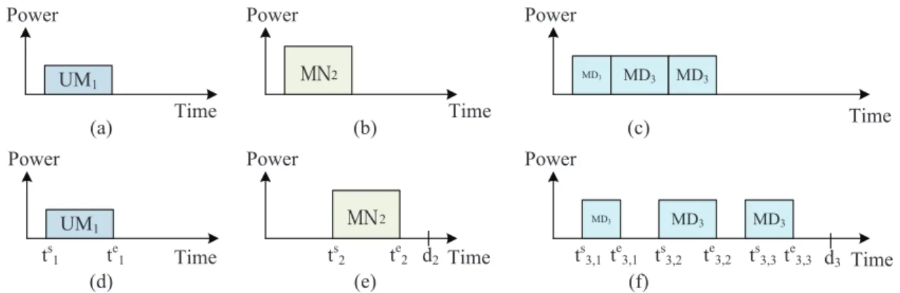
Figure 3.1: An example of electric appliance types. (a), (b), and (c) are three appliances before scheduling. (d), (e), and (f) are three appliances after scheduling.

For each electric appliances of MD typeMDl, l = 1 . . . z, the execution time can be

divided inton parts. For u = 1 . . . n, each part start at time ts

l,u and end at timet e l,u. All

parts must execute before deadlinedM D

l by increasing order. The power consumption of

MDl at timet is pM Dl (t). For example, washers, water pumps, and battery chargers are

electric appliances of MD type.

Fig. 3.1 shows an example of these appliances. Fig. 3.1(a), Fig. 3.1(b), and Fig. 3.1(c) are UM type, MN type, and MD type appliances before scheduling, respectively. The execu-tion time ofUM1 can not be moved. As shown in Fig. 3.1(d), the execution time is same as

Fig. 3.1(a). The execution time ofMN2 can be moved. As shown in Fig. 3.1(e), after

schedul-ing, theMN2 starts fromts2 tot e

2. The execution time ofMD3 can divided into three parts. As

shown in Fig. 3.1(f), after scheduling, theMD3 starts from [ts3,1,te3,1], [ts3,2,te3,2], and [ts3,3,te3,3].

The total power consumption of all above electric appliances can not be exceeded the upper bound thresholdδ at any time t, i.e.,

Σ∀iγi+ Σ∀jpU Mj (t) + Σ∀kpM Nk (t) + Σ∀lpM Dl (t) ≤ δ

In our scenario, the cost of power consumptionc(t) may be different at different time. Hence,

our goal is to adjust the execution time of each appliance to minimize the total cost, i.e.,

min{ Z te j ts j fj(t)c(t)dt + Z te k ts k gk(t)c(t)dt + n X u=1 Z te l,u ts l,u hl(t)c(t)dt}

Figure 3.2: The flow chart of iPM system.

MN

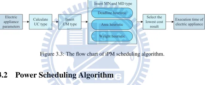
Figure 3.3: The flow chart of iPM scheduling algorithm.

3.2

Power Scheduling Algorithm

Our iPM system can schedule the executing electric appliances dynamically. Fig. 3.2 shows the flow chart of our iPM system. Users should set the parameters about electric appliances, such as start time, end time, deadline, etc. Then, control server will read these configurations and compute these electric appliances power consumption dynamically. According to above parameters of electric appliances, we design a power scheduling algorithm to schedule these electric appliances. Then, these electric appliances will execute by the scheduling result. When an new electric appliance enters the system or an electric appliance terminates, the control server will redo the power scheduling algorithm to guarantee minimizing the total cost for all electric appliances.

Here, we propose a scheduling algorithm for executing electric appliances. Fig. 3.3 shows the flow chart of scheduling algorithm. At first, we consider the electric appliances of UC type. Then, we insert electric appliances of UM type. After that, we propose three heuristic methods

Power

Time

MN MD

Cost

tref1 tref2 tref3 tref4 tref5

c(t)

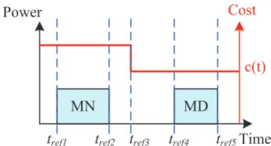
Figure 3.4: An example of the reference points.

from above three heuristic methods. For greedy approaches in heuristic methods, we define two metrics, which are the areas and weighted values of the electric appliances. The area of an electric appliance is the total power consumption while executing. For the electric appliances of MN and MD types, the areas can be denoted as following.

area(MNk) = Z te k ts k gk(t)c(t)dt area(MDl) = n X u=1 Z te l,u ts l,u hl(t)c(t)dt

Besides, the weighted values are denoted as the area divided by available time, i.e.,

weight(MNk) = area(MNk)/(dk− tnow)

weight(MDl) = area(MDl)/(dl− tnow)

Before describing the detail of the scheduling algorithm, we define the reference time point for inserting the electric appliances of MN and MD types.

Definition 1 The reference time point tref is a time point that satisfies one of the following

constraints.

• The boundary of the cost of power consumption, i.e., c(tref + ω) 6= c(tref) and c(tref −

ω) 6= c(tref), where the ω is a constant.

• The start time or end time of electric appliances of UM type, i.e., the tref = tsjortref = tej

for allj = 1 . . . x in UMj.

• The start time or end time of electric appliances of MN type, i.e., the tref = tskortref = tek

• The start time or end time of electric appliances of MD type, i.e., the tref = tsl,u or

tref = tel,ufor alll = 1 . . . z and u = 1 . . . n in MDl.

Fig. 3.4 shows an example of the reference time points. The left and right x-axis are the power consumption of electric appliances and the cost of power consumption, respectively. There are five reference time points in this example. The time pointtref 1 andtref 2are the start and end

time of electric appliances of MN type, respectively. The time pointtref 4andtref 5are the start

and end time of electric appliances of MD type, respectively. Thetref 3is the boundary of cost

of power consumption.

Our proposed power scheduling algorithm is composed of the following steps:

SchedulingEA(UC, UM, MN, MD, δ)

1. Subtract the power consumption ofUCifori = 1 . . . w from δ, i.e., δ = δ − Σ∀iγi.

2. InsertUMj forj = 1 . . . x by their tsj andtej.

3. Get current reference time pointstrefr, wherer = 1 . . . m.

4. Try to schedule allMNkandMDlby following three heuristic methods individually and

calculate their cost while executing.

• Deadline heuristic: Sort MNk andMDlfork = 1 . . . y and l = 1 . . . z according to

dkanddlby increasing order into a setEA. Then, do InsertEA(EA) to insert these

electric appliances.

• Area heuristic: Sort MNk and MDl for k = 1 . . . y and l = 1 . . . z according

to area(MNk) and area(MDl) by decreasing order into a set EA. Then, do

InsertEA(EA) to insert these electric appliances.

• Weight heuristic: Sort MNk and MDl for k = 1 . . . y and l = 1 . . . z according

toweight(MNk) and weight(MDl) by decreasing order into a set EA. Then, do

InsertEA(EA) to insert these electric appliances.

5. Choose the lowest cost result of above three heuristics to execute.

InsertEA(EA)

(a) Ifea is MD type, greedily and sequentially insert each parts of ea into the trefr with

the lowest cost, i.e., min∀r{c(trefr)} and satisfy the δ and deadline constraints. If

multipletrefr can be chosen, choose the the latest time first.

(b) Otherwise, greedily insert ea into a trefr with the lowest cost, i.e.,min∀r{c(trefr)}

and satisfy the δ and deadline constraints. If multiple trefr can be chosen, choose

the the latest time first.

Fig. 3.5 shows an example of the power scheduling algorithm. As shown in Fig. 3.5(a), theUC1 electric appliance withγ1 = 2 and UM1 electric appliance withts1 = 4 and te1 = 6.

TheMN1 andMN2 electric appliances with respectively. TheMD1 electric appliance can be

divided into two parts withdM D

1 = 16. At first, we consider the UC1 and UM1. As shown

in Fig. 3.5(b), the δ is 4 after scheduling the UC1. By deadline heuristic, we insert MN2,

MN1, andMD1 sequentially in Fig. 3.5(c1), Fig. 3.5(c2), and Fig. 3.5(c3), respectively. By

area heuristic, we insertMD1, MN1, andMN2 sequentially in Fig. 3.5(d1), Fig. 3.5(d2), and

Fig. 3.5(d3), respectively. By weight heuristic, we insertMN1, MN2, andMD1 sequentially

in Fig. 3.5(e1), Fig. 3.5(e2), and Fig. 3.5(e3), respectively. In the example, the lowest cost one is deadline heuristic.

Power Cost Time 5 5 4 8 12 0 MN1 MD1,1 MD1,2 MN2 UM1 Power Cost Time 5 5 4 8 12 0 Power Cost Time 5 5 4 8 12 0 Power Cost Time 5 5 4 8 12 0 Power Cost Time 5 5 4 8 12 0 Power Cost Time 5 5 4 8 12 0 Power Cost Time 5 5 4 8 12 0 Power Cost Time 5 5 4 8 12 0 Power Cost Time 5 5 4 8 12 0 Power Cost Time 5 5 4 8 12 0 Power Cost Time 5 5 4 8 12 0 dMN=10 dMN₌₈ ts=4 te=6 dMD=16 UM1 UM1 UM1 UM1 MN2 UM1 MN2 MN1 UM1 MN2 MN1 MD1,1MD1,2 MD1,1MD1,2 UM1 MD1,1MD1,2 MN1 MN2 UM1 MN1 MD1,1MD1,2 MN2 UM1 MN1 MN2 UM1 MN1 MD1,1MD1,2 MN1 (a) (b) (c2) (c1) (c3) (d2) (d1) (d3) (e2) (e1) (e3) 1 1 1 2 1 Ȣ=2₁

Figure 3.5: An example of power scheduling algorithm. (a) The parameters of the example. (b) Scheduling result after insertUC and UM types. (c) Scheduling results by deadline heuristic.

Chapter 4

Prototyping Results

4.1

Hardware Components

The hardware components of iPM system can be divided into two parts, i.e., wireless power meter and sink receiver. Fig. 4.1 shows our wireless power meter. It is composed of three units: 1. Power sensing unit: We adopt ADE7763 [1] as our energy meter IC to get the energy consumption of electric appliances. As shown in Fig. 4.2, the electric current and voltage can be gotten by current transformer and transformer via channel-1 (CH1) and channel-2 (CH2), respectively. Then, we can get power consumption of electric appliances via SPI (serial peripheral interface).

2. Control unit: Fig. 4.1 shows the control unit of our wireless power meter. We adopt Atmel AVR ATmega128 [2] as our microcontroller which can get power consumption via serial peripheral interface and transmit data via UART interface. Besides, we provide three relay for power control and mode switch.

3. Wireless transmission unit: As shown in Fig. 4.1, we adopt Jennic JN5148 [4], which is a single-chip microprocessor compatible with IEEE 802.15.4 [13], as our wireless trans-mission module. Through the UART interface, it can get the statuses of electric appliances and transmit to our control server.

Fig. 4.4 shows our sink receiver. We adopt Jennic JN5148 [4] as our wireless transmission mod-ule and adopt FTDI FT232RL [3] to translate UART interface to USB interface from JN5148. So, the control server can get data form electric appliances or send commands to electric appli-ances via USB interface.

Figure 4.1: The hardware components of our wireless power meter.

Figure 4.3: Hardware component of power sensing unit. (a) (b) Jennic JN5148 FDT232RL UART USB Regulators 3.3v

Figure 4.4: The hardware component of iPM system. (a) The hardware components of our sink receiver. (b) Our implemented sink receiver.

Hardware

Server

Power Control Equipment Mode Control Energy Metering IC ZigBee Network Interface Power Scheduling Algorithm Graphic User

Interface ZigBee Network

Device controller

Wireless power meter

Command Decoder Noise Filter UART, SPI Interface Processing

Software

4.2

Software Components

Fig. 4.5 shows our functional block of implementation. In wireless power meter, four device controller modules send command and receive data from hardware components. The relay and output I/O controller can control the power and modes of electric appliances, receptively. The meter and network controller can get and send metering data to control server, respectively. Before sending the metering data to control server, we preprocess these data by noise filter to get more precision metering data. Beside, for ease of programming, we design some commands to communicate between wireless power meter and control server. The command decoder can decode command to do suitable actions. As shown in Fig. 4.6, in control server, we provide a graphic user interface to set and monitor whole system status. Also, we log all metering data from wireless power meter into a database system.

Chapter 5

Simulation Results

In this section, we present some simulation results to evaluate the system performance. We consider the power consumption of a house with a set of eleven electric appliances, where one is UC type, three are UM type, six are MN type, and the other is MD type. One hundred electric appliances are generated randomly from the set and inserted into different time slots during the simulation time. Table 5.1 lists the electric appliances set of our simulator. We set the instantaneous power threshold to 500 watt-second, and the simulation time is set to 168 hours (a week). In order to observe different scheduling results, we set the electric price is fluctuating every three hours as shown in Fig. 5.1.

We compare our iPM system with the non-schedule system in our iPM simulator to observe the power consumption and monetary cost. We define the power consumption as the accu-mulative power of the simulation time, and the monetary cost as the total cost of the power consumption.

The power consumption of our iPM system is similar to that of the non-schedule system as shown in Fig. 5.2. It is because all electric appliances are working well after scheduling. Fig. 5.3 shows the instantaneous power during the simulation time. However, we find that the instantaneous power of our iPM system, with the three heuristic methods, is more evenly stable than that of the non-schedule system. Even though some power loads can not be shifted from the peak time, the power load would never exceed the power threshold after scheduling.

With regard to monetary cost, iPM can save more. Customers can decide which heuristic method they want, or they may use the default setting, choosing the lowest cost from these three heuristic methods. From Fig. 5.4, we can find that iPM can save 24.5% cost less than the non-schedule system.

Table 5.1: The electric appliance set

Type Execution time Deadline after start Power consumption (minute) (minute) per watt-second UC Uncontrollable Uncontrollable 30 UM 30 Uncontrollable 80 UM 40 Uncontrollable 60 UM 50 Uncontrollable 70 MN 50 360 70 MN 60 360 90 MN 70 360 45 MN 35 720 120 MN 20 720 120 MN 120 720 50 MD 110 720 50 45 720 35 0 0.5 1 1.5 2 2.5 0 20 40 60 80 100 120 140 160 Cost Simulation time

0 50000 100000 150000 200000 250000 300000 350000 400000 450000 0 5 1 0 1 5 2 0 2 5 3 0 3 5 4 0 4 5 5 0 5 4 5 9 6 4 6 9 7 4 7 9 8 4 8 9 9 4 9 9 1 0 4 1 0 9 1 1 4 1 1 9 1 2 4 1 2 9 1 3 4 1 3 9 1 4 4 1 4 9 1 5 3 1 5 8 1 6 3 Accu mu la ti ve P o w e r Time (hour) Non-schedule Deadline 0 50000 100000 150000 200000 250000 300000 350000 400000 450000 0 5 1 0 1 5 2 0 2 5 3 0 3 5 4 0 4 5 5 0 5 4 5 9 6 4 6 9 7 4 7 9 8 4 8 9 9 4 9 9 1 0 4 1 0 9 1 1 4 1 1 9 1 2 4 1 2 9 1 3 4 1 3 9 1 4 4 1 4 9 1 5 3 1 5 8 1 6 3 Ac cum ula tiv e P o w e r Time (hour) Non-schedule Area 0 50000 100000 150000 200000 250000 300000 350000 400000 450000 0 5 1 0 1 5 2 0 2 5 3 0 3 5 4 0 4 5 5 0 5 4 5 9 6 4 6 9 7 4 7 9 8 4 8 9 9 4 9 9 1 0 4 1 0 9 1 1 4 1 1 9 1 2 4 1 2 9 1 3 4 1 3 9 1 4 4 1 4 9 1 5 3 1 5 8 1 6 3 Ac cum ula tiv e P o w e r Time (hour) Non-schedule Weight 0 50000 100000 150000 200000 250000 300000 350000 400000 450000 0 5 1 0 1 5 2 0 2 6 3 1 3 6 4 1 4 6 5 1 5 6 6 1 6 6 7 1 7 7 8 2 8 7 9 2 9 7 1 0 2 1 0 7 1 1 2 1 1 7 1 2 2 1 2 8 1 3 3 1 3 8 1 4 3 1 4 8 1 5 3 1 5 8 1 6 3 Accu mu la ti ve P o w e r Time (hour) Non-schedule Incorpartion (a) (b) (c) (d)

Figure 5.2: The accumulative power of (a) Deadline heuristic, (b) Area heuristic, (c) Weight heuristic, and (d) incorporation.

0 20 40 60 80 1 0 0 1 2 0 1 4 0 1 6 0 1 8 0 2 0 0 1 39 77 115 153 191 229 267 305 343 381 419 457 495 533 571 609 647 685 723 761 799 837 875 913 951 989 1027 1065 1103 1141 1179 1217 1255 1293 1331 1369 1407 Power (W) T ime (h o u r) N o n -s c h e d u le D e a d lin e 0 50 1 0 0 1 5 0 2 0 0 2 5 0 3 0 0 1 39 77 115 153 191 229 267 305 343 381 419 457 495 533 571 609 647 685 723 761 799 837 875 913 951 989 1027 1065 1103 1141 1179 1217 1255 1293 1331 1369 1407 Power (W) T ime (h o u r) N o n -s c h e d u le A rea 0 50 1 0 0 1 5 0 2 0 0 2 5 0 3 0 0 1 39 77 115 153 191 229 267 305 343 381 419 457 495 533 571 609 647 685 723 761 799 837 875 913 951 989 1027 1065 1103 1141 1179 1217 1255 1293 1331 1369 1407 Power (W) T ime (h o u r) N o n -s c h e d u le W e ig h t 0 20 40 60 80 1 0 0 1 2 0 1 4 0 1 6 0 1 8 0 2 0 0 1 39 77 115 153 191 229 267 305 343 381 419 457 495 533 571 609 647 685 723 761 799 837 875 913 951 989 1027 1065 1103 1141 1179 1217 1255 1293 1331 1369 1407 Power (W) T ime (h o u r) N o n -s c h e d u le In c o rp a rti o n (a) (b ) (c) (d ) F ig u re 5 .3 : T h e p o w er o f (a ) D ea d lin e h eu ris tic , (b ) A re a h eu ris tic , (c ) W ei g h t h eu ris tic , an d (d ) in co rp o ra tio n d u rin g th e si m u la tio n tim e. 2 1

0 100000 200000 300000 400000 500000 600000 700000 0 4 9 1 3 1 8 2 2 2 7 3 1 3 5 4 0 4 4 4 9 5 3 5 8 6 2 6 7 7 1 7 5 8 0 8 4 8 9 9 3 9 8 1 0 2 1 0 6 1 1 1 1 1 5 1 2 0 1 2 4 1 2 9 1 3 3 1 3 7 1 4 2 1 4 6 1 5 1 1 5 5 1 6 0 1 6 4 C o st Time (hour) Non-schedule Deadline Area Weight Incorpartion

Chapter 6

Conclusions

In this paper, we propose an intelligent power scheduling system (iPM) based on pervasive meters. Each electric appliance connects to a wireless power meter. Through these wireless meters, the current power consumption of electric appliances can be transmitted to the control server. Our goal is to dynamically schedule the execution time of each electric appliance in a home to minimize the total monetary cost. Still, it poses several challenges: 1) user demand response, 2) load management, and 3) minimizing the monetary cost of electricity consumption. Hence, we propose a power scheduling algorithm for smart usage of electric appliances in a home dynamically. We verify our results through simulations as well as a real prototype. Specifically, we develop a power scheduling system based on the ZigBee Smart Energy Profile to monitor and schedule the usage of electric appliances.

Bibliography

[1] ADE7763: Single-phase active and apparent energy metering ic. http://www.analog.com/. [2] Atmega128. http://www.atmel.com/.

[3] FTDI FT232RL USB to Serial Chip. http://www.parallax.com/. [4] Jennic, JN5148. http://www.jennic.com/.

[5] WorldBank. http://data.worldbank.org/. [6] ZigBee alliance. http://www.zigbee.org/.

[7] C. Babu and S. Ashok. Peak load management in electrolytic process industries. IEEE

Power Systems, 23(2):399–405, 2008.

[8] S. Y. Chan, S. W. Luan, J. H. Teng, and M. C. Tsai. Design and implementation of a rfid-based power meter and outage recording system. In Proc. of IEEE International

Conference on Sustainable Energy Technologies, 2008.

[9] A. I. Cohen and C. C. Wang. AN OPTIMIZATION METHOD FOR LOAD MANAGE-MENT SCHEDULING. IEEE Power Systems, 3(2):612–618, 1988.

[10] A. Cuevas, C. Lastres, J. Caffarel, R. Martizez, and A. Santamaria. Next generation of energy residential gateways for demand response and dynamic pricing. In Proc. of IEEE

Int’l Conference on Consumer Electronics (ICCE), 2011.

[11] H. Farhangi. The path of the smart grid. IEEE Power and Energy Magazine, 8:18–25, 2010.

[13] IEEE standard for information technology - telecommunications and information ex-change between systems - local and metropolitan area networks specific requirements part 15.4: wireless medium access control (MAC) and physical layer (PHY) specifications for low-rate wireless personal area networks (LR-WPANs), 2003.

[14] A. Ipakchi and F. Albuyeh. Grid of the future. IEEE Power and Energy Magazine, 7:56– 62, 2009.

[15] Y. Kim, T. Schmid, Z. M. Charbiwala, and M. B. Srivastava. ViridiScope: design and implementation of a fine grained power monitoring system for homes. In Proc. of ACM

Int’l Conference on Ubiquitous computing (Ubicomp), 2009.

[16] G. Strbac. Demand side management: Benefits and challenges. Energy Polocy, 36:4419– 4426, 2008.

[17] U. Sulayman and A. T. Alouani. Smart grid monitoring using local area sensor network. real-time data acquisition, analysis and management. In Proc. of IEEE Southeastcon, pages 444–449, 2011.

[18] Z. Xi, W. Xiong, S. Wang, and W. Huang. Study on electricity sub-metering system of campus. In Proc. of Asia-Pacific Power and Energy Engineering Conference (APPEEC), pages 1–4, 2011.

[19] J. Xiong, T. L. Wang, and Y. Chao. The design of tiered pricing meter based on zig-bee wireless meter reading. In Proc. of Int’l Conference on Measuring Technology and