調控式的部份最小平方法之研究

國

立

交

通

大

學

多媒體工程研究所

碩

士

論

文

調 控 式 的 部 份 最 小 平 方 法 之 研 究

Study on Partial Regularized Least Squares Method

研 究 生：邱郁仁

指導教授：蕭子健

調 控 式 的 部 份 最 小 平 方 法 之 研 究

Study on Partial Regularized Least Squares Method

研 究 生：邱郁仁 Student : Yu-Ren Chiou

指導教授：蕭子健 Advisor：Tzu-Chien Hsiao

國 立 交 通 大 學

多 媒 體 工 程 研 究 所

碩 士 論 文

A Thesis

Submitted to Institute of Computer Science and Engineering College of Computer Science

National Chiao Tung University in partial Fulfillment of the Requirements

for the Degree of Master

in

Computer Science

July 2008

Hsinchu, Taiwan, Republic of China

調控式的部份最小平方法之研究

研 究 生：邱郁仁

指導教授：蕭子健

國 立 交 通 大 學

多 媒 體 工 程 研 究 所

摘要

本論文的目的在於建構一種分析法則，在未經處理的原始資料去除不必要的 隱藏訊息。此新的學習法則稱之調控式的部份最小平方法，是合併部份最小平方 法和規律法的優點，即使在雜訊的資料下，可避免過度配適的現象，得到較好的 估算結果。 在模擬數據分析部份，調控式部份最小平方法用來分析三種不同的波型，並 以均方根誤差做為判定的標準說明調控式部份最小平方法可得到較好的結果;實 際的測量數據分析部份，利用實際的聲音檔案以及血糖濃度的光譜資料來驗證所 提出的調控式部份最小平方法的確具備去除雜訊能力。 i

Study on Partial Regularized Least Squares Method

Student：Yu-Ren Chiou

Advisor：Tzu-Chien Hsiao

Institute of Computer Science and Engineering College of Computer

Science

National Chiao Tung University

Abstract

The main purpose of this thesis is to develop a method of analyzing and reducing the unseen or noisy information from the source data without preprocessing. Here presents a novel learning algorithm—partial regularized least squares (PRLS). It combines the advantages of both the partial least squares (PLS) and regularization technique to provide an efficient procedure to avoid the circumstance of overfitting and attain better results when calibrating under noisy data.

In the simulated experiments, PRLS is applied to analyze the three different kinds of simulated waves. According to estimated standard of root mean square error, proving that PRLS has better performance than PLS. In real calibrated experiments, demonstrating PRLS certainly has the ability of noise reduction.

Acknowledgement

First of all, I would like to express my sincere appreciation to my advisor, Dr. TC Hsiao, for his helpful guidance, careful supervision and encourage throughout my Master degree. Under his guidance, he shows me a way how to treat and analyze the problem. And also thanks for Prof. Lin, as his professional approval that I have successfully adopt environment sound data for testing the performance of proposed scheme.

In the past of two years, he has stimulated the research work and also offered an excellent research environment at the VBM laboratory. I would also express my gratitude to all the members in the VBM laboratory, for their encouragements, assistances, useful suggestions and comments. I am grateful to all of my friends for their supports and encouragements. You have made my life wonderful and cheerful.

Finally, thank my family for their understanding, supports and loves. Life is sometimes tough; however, there is nothing to defeat us with loves of family.

Contents

Chinese abstract………... i Abstract……… ii Acknowledgement……… iii Contents………... iv List of Figures………... vi List of Tables……….. ix Chapter 1. Introduction……… 1 1.1. Literature study………... 1 1.2. Motivation….…..………... 2 1.3. Related work………….……….. 2 1.4. Contributions……….. 4 1.5. Thesis Organization……… 4

Chapter 2. Methods and Materials………..………. 5

2.1. Least Squares (LS)………...………... 5

2.2. Principal Component Analysis (PCA)……… 7

2.3. Partial Least Squares (PLS)……… 8

2.4. Orthogonal Least Squares (OLS)……… 10

2.5. Regularization………. 12

2.6. Regularized Orthogonal Least Squares (ROLS)………. 13

Chapter 3. A novel method-Partial Regularized Least Squares (PRLS)………..… 15

3.1. Relation between PLS and regularization………... 15

3.2. PRLS algorithm…………... 16

Chapter 4. Experiments and discussion………... 18

4.1. Illustration………... 18

4.1.1. Synthesized simulation data………. 18

4.1.2. Criterion of estimation………. 19 4.1.3. Conditional training………. 20 4.2. Simulation data ……….. 21 4.2.1. Sigmoid function………….………. 21 4.2.2. Polynomial function.……… 26 4.2.3. Imitative spectrum……… 30 iv

4.2.4. Discussion………. 34

4.3. Real data……….. 35

4.3.1. Sound data……… 35

4.3.2. Blood Glucose data……….. 40

4.3.3. Discussion……… 44

Chapter 5. Conclusion and future works……….. 46

5.1. Conclusion……….. 46

5.2. Future works..………. 46

References……… 47

List of Figures

Figure 1.1 Research tracing diagram………... 1

Figure 1.2 Illustration of overfitting……… 3

Figure 2.1 Two layer LS architecture.………. 6

Figure 2.2 Illustration of LS in geometry……… 6

Figure 2.4 Singular value decomposition of covariance matrix……….. 7

Figure 2.5 Three layer PCA architecture……….… 8

Figure 2.6 PLS algorithm flow chart………... 9

Figure 2.7 Three layer PLS architecture……….. 10

Figure 2.8 OLS based on RBFN flow chart……….…… 11

Figure 2.9 Three layer OLS architecture……….………. 12

Figure 2.10 Three layer ROLS architecture……….… 14

Figure 3.1 Trade off curve………... 16

Figure 3.2 PRLS algorithm flow chart………. 17

Figure 3.3 Three layer PRLS architecture……… 17

Figure 4.2 A sketch map of correlation coefficient……….. 19

Figure 4.3 Root mean square error………... 20

Figure 4.4 Self-calibration & self-prediction (SCSP)……….. 21

Figure 4.5 Cross validation (CV)………. 21

Figure 4.6 Noisy training data (points) and sigmoid function (curve) with N/S ratio = 0.55 (sigmoid function)….………... 22

Figure 4.7 Correlation coefficient as a function of N/S ratio under SCSP (sigmoid function)……….. 23

Figure 4.8 RMSE as a function of N/S ratio under SCSP (sigmoid function)……... 23

Figure 4.9 Network mapping constructed by PRLS and PLS algorithm under SCSP with N/S ratio = 0.55 (sigmoid function)……….…... 24

Figure 4.10 Correlation coefficient as a function of iteration under CV (sigmoid function)………... 24

Figure 4.11 RMSE as a function of iteration under CV (sigmoid function)……… 25

Figure 4.12 Network mapping constructed by PRLS and PLS algorithm under CV with N/S ratio = 0.55 (sigmoid function)………..……..….. 25

Figure 4.13 Noisy training data (points) and polynomial function (curve) with

N/S ratio = 0.55 (polynomial)……….…. 26 Figure 4.14 Correlation coefficient as a function of N/S ratio under SCSP

(polynomial)……….….... 27 Figure 4.15 RMSE as a function of N/S ratio under SCSP

(polynomial)………..……... 27 Figure 4.16 Network mapping constructed by PRLS and PLS algorithm under

SCSP with N/S ratio = 0.55 (polynomial)………….……….. 28 Figure 4.17 Correlation coefficient as a function of N/S ratio under CV

(polynomial)………. 28 Figure 4.18 RMSE a function of N/S ratio under CV (polynomial)……… 29 Figure 4.19 Network mapping constructed by PRLS and PLS algorithm under

CV with N/S ratio = 0.55 (polynomial)………... 29 Figure 4.20 Linear combination of two Gaussian functions with different mean

and standard deviation………. 30 Figure 4.21 Training data sets of imitative spectrum………... 31 Figure 4.22 Correlation coefficient as a function of executable iteration under

SCSP (imitative spectrum)……….………….……. 31 Figure 4.23 RMSE as a function of executable iteration under SCSP (imitative

spectrum)……….…. 32 Figure 4.24 Network mapping constructed by PRLS and PLS algorithm under

SCSP with N/S ratio = 0.55 (imitative spectrum)……… 32 Figure 4.25 Correlation coefficient as a function of executable iteration under

CV (imitative spectrum)……….……….…. 33 Figure 4.26 RMSE as a function of executable iteration under CV (imitative

spectrum)……….. 33 Figure 4.27 Network mapping constructed by PRLS and PLS algorithm under

CV with N/S ratio = 0.55 (imitative spectrum)……….……….…. 34 Figure 4.28 Power station ambience source data……….… 35 Figure 4.29 Correlation coefficient as a function of index of hidden node under

SCSP (power station ambience)………... 36 Figure 4.30 RMSE as a function of index of hidden node under SCSP (power

station ambience)………. 36 Figure 4.31 Correlation coefficient as a function of index of hidden node under

CV (power station ambience)……….. 37 Figure 4.32 RMSE as a function of index of hidden node under CV (power

station ambience)………. 37 Figure 4.33 Transformer hum source data………... 38 Figure 4.34 Correlation coefficient as a function of index of hidden node under

SCSP (transformer hum)……….. 38 Figure 4.35 RMSE as a function of index of hidden node under SCSP

(transformer hum)……… 39 Figure 4.36 Correlation coefficient as a function of index of hidden node under

CV (transformer hum)……….………. 39 Figure 4.37 RMSE as a function of index of hidden node under CV (transformer

hum)………. 40 Figure 4.38 Blood glucose data with noise……….. 41 Figure 4.39 Correlation coefficient as a function of executable iteration under

SCSP (blood glucose)……….. 41 Figure 4.40 RMSE as a function of executable iteration under SCSP (blood

glucose)……….... 42 Figure 4.41 Network mapping constructed by PRLS and PLS algorithm under

SCSP (blood glucose)……….. 42 Figure 4.42 Correlation coefficient as a function of executable iteration under

CV (blood glucose)……….. 43 Figure 4.43 RMSE as a function of executable iteration under CV (blood

glucose)……… 43 Figure 4.44 Network mapping constructed by PRLS and PLS algorithm under

CV (blood glucose)………..……….... 44

ix

List of Tables

Table 4.1 Optimal CV results for sigmoid function data………... 25

Table 4.2 Optimal CV results for polynomial prediction data………. 29

Table 4.3 Optimal CV results for imitative spectrum prediction data………. 34

Table 4.4 Compilation of simulated experimental results………... 35

Table 4.5 Optimal CV results for power station ambience prediction data………. 38

Table 4.6 Optimal CV results for transformer hum prediction data……… 40

Table 4.7 Optimal CV results for blood glucose data……….. 44

~1L3t~*~

1ilf

1G

pJT

iJ~

±

fJI

Study on Partial Regularized Least Squares Method

;f§

~~~~

:

---<---"-- \ -_ _---'-- _

it. :

Institute of Multimedia and Engineering

College of Computer Science

National Chiao Tung University

Hsinchu

,

Taiwan, R.O.C.

As members of the Final Examination Committee

,

we certify that

we have read the thesis prepared b

y

Yu-Ren Chiou

entitled Study on Partial Regularized Least Squares Method

and recommend that it be accepted as fulfilling the thesis

requirement for the Degree of Master of Science.

Committee Members:

l

U h

-

H

"

t

ot

ft/

c

~

711 '

J

~

(l

Director:

Chapter 1. Introduction

1.1. Literature study

Multivariate analysis is successfully applied to process signal information. The application field includes spectrum analysis [1], bio-signal process [2] and image processing [3] etc. In general, it can be divided into two categories: regressor and value iteration also named as artificial neural network (ANN). The wildly used regressors are: Least Squares (LS), Principal Component Analysis (PCA) [4] and Partial Least Squares (PLS) [5]. And the most practical model in ANN is Multiple Layer Perceptron (MLP) [6]. Regressor and ANN analyze data in different processes and the analyzed results are suitable for different applications. For example, Wang [7] used ANN to solve the problem, classification of oral submucous fibrosis and oral carcinogenesis. Hsiao [8] apply regressor to classify the difference between normal and dyplasia tissues.

Hsiao [9] proposed a novel thought to hybrid regressive algorithm and ANN. In his study, the regressive algorithms can be treated as ANN architecture. For example, PLS can be treated as a three-layer ANN. For this view point, the research tracing path in this thesis will be illustrated in Figure 1.1.

Similar architecture ROLS

Regularization

ANN

OLS based on RBFN Multi-Layer Perceptron LS PCA PLS

Regressor

PRLS

Regularization

Similar architecture ROLS

Regularization

ANN

OLS based on RBFN Multi-Layer Perceptron LS PCA PLS

Regressor

PRLS

Regularization

Figure 1.1 Research tracing diagram

Oja [4], [10] proposed PCA to reduce the dimension of input data by K-L transformation. However it has a main drawback which PCA lacks for information about which principal components are important for desired output and how many components are needed to compress the input data. PLS is a calibrated regression in common use. The concept of PLS was developed from LS. PLS also can compress the input data and solve the main drawback of PCA. But PLS estimation suffers from overfitting is more serious than PCA [5]. Chen [11] proposed Orthogonal Least Squares (OLS) based on radial basis function network (RBFN) also suffered from the same circumstance. By applying the regularization technique, Chen [12] also constructed Regularized Orthogonal Least Squares (ROLS) to solve the problem of overfitting.

In order to apply regularization technique to PLS, we represent PLS as three layer network. Following the example of ROLS computational architecture, we also modify the original PLS by combining the regularization to establish a novel calibrated model – partial regularized least squares (PRLS).

1.2. Motivation

PLS is a multivariate statistical technique that allows comparison between multiple response variables and multiple explanatory variables. It has been popular in many aspects. However there is a big problem that the predicted results would be influenced by outlier hidden in training data and lapse from output. The position is due to overtraining of system because we hope that executed outputs can approximate to desired outputs as far as possible. In ideal data, calibrated outcomes will be perfect but real data sets always have unseen information so that some results may reflect anomalies due to the information and poor accuracy for unseen examples. When training data goes along with noise, prediction often falls into a trap – overfitting [13]. Therefore we want to modify a usual method to acquire better performance than the original one when calibrating under noisy training data.

1.3. Related work

Pervious approaches have been proposed to solve the problem of overfitting.

Figure 1.2 Illustration of overfitting.

The learner may adjust to specific features of the noisy training data that has no causal relation to calibration. To reduce the training error, the predicted curve would pass through each point possibly. At the same time, results would be influenced by the data with noise.

In general, three common techniques are selected to do:

1. Halt early – System would terminate training under a tolerant threshold. It is the simplest method but we have no idea when system must stop executing. If calculation process is terminated too early, results will be underfitting. Hence, it is difficult to determine when stopping working [6].

2. Postprocessing – System would select a validation data from original training data set and repeat until each observation in the set is used as validation data. The method also has the property of avoiding overfitting but it costs a large amount of computation [14].

3. Regularization – System would adopt iterative learning and calculate the probability distribution and acquiring the balance between overfitting and underfitting [12], [15], [16], [17], but it is hard to select regularized parameters appropriately.

1.4. Contribution

The contributions of this thesis can be summarized into two levels, as follow: 1. Here established a novel method combines a usual regression model with

regularization, named PRLS. It combines the advantages of PLS and regularization.

2. Here also improved the accuracy of being calibrated by using PLS under the influence of noisy training data.

1.5. Thesis organization

Chapter 2 introduces the principle and architecture of several calibration models and further traces regularization technique [16], [17]. In Chapter 3, we discuss the relationship between PLS and regularization. Next, we propose a novel model - PRLS built by combining PLS with the technique. Chapter 4 shows the simulated experimental results of our purpose to evidence our theory. At last, the conclusion and further works are written down in Chapter 5.

Chapter 2. Methods and Materials

2.1. Least Squares (LS)

Classical least squares regression consists of minimizing the sum of the squared

residuals. The linear model is given byy_i =b₀+x_i1b₁+...+x_ipb_p+

ε

_i ( i = 1,…,n ), where the error ε_i is usually assumed to be normally distributed with zero mean and standard deviation σ. The goal of multiple regression is to estimate

from the data . The sum of square error (SSE) is calculated as below: ) ,..., , (b₀ b₁ b_p b= ) , ,..., , 1 ( x_i1 x_ip y_i 2 (2-1) 1 1 1 0 1 2 _{( ( ... ))} p ip n i i i n i i y b x b x b SSE

∑

∑

= = + + + − = = ε

Partial difference by

b

_j, then we can derive (2-2)

∑

−

+

+

+

−

=

=

∂

∂

= n i i i ip p ij j

x

b

x

b

x

b

y

b

SSE

1

(

(

0 1 1

...

))(

1

)

0

2

(2-2) where j = 1,2,…,p.

If we transform to matrix form, we can get a two layer multivariate analysis system illustrated as Figure 2.1. Then Y represents as matrix

[

y₁,..., y_n

]

T , real output

and .

T 1

,...,

]

[

y

y

_n

Y

∧

=

∧ ∧ b=[b₀,b₁,...,b_p] The LS procedure in matrix form is defined as:

y

=

X

b

+

ε

(2-3) We calculate the weighting coefficients due to (2-3).

b y X X XT _≈ T (2-4) ) (X X) (X y b _≈ T −1 T (2-5) - 5 -

∑

∧

y

p

x

1

x

0

x

₂

...

b

b

₁

b

_p

∑

∑

∧

y

p

x

1

x

0

x

₂

...

b

b

₁

b

_p

Figure 2.1 Two layer LS architecture.

In other words, LS method is to solve the approximated answer if there is no solution in geometry. We will use Figure 2.2, so as to explain

Figure 2.2 Illustration of LS in geometry

If express the column vectors of can not span the vector . We define the vector space because the equation

b X Y ≠ X Y )) ( ( X

W = span col Y ≠ Xbimplies there is no

solution. If we want to obtain the approximated answer, we have to reduce the residual ε . By the orthogonal projecting into vector space acquiring the approximation because vector goes to space takes straightly being apart from as the shortest. W Y W

b

X

y

W

ε

- 6 -

2.2. Principal Component Analysis (PCA)

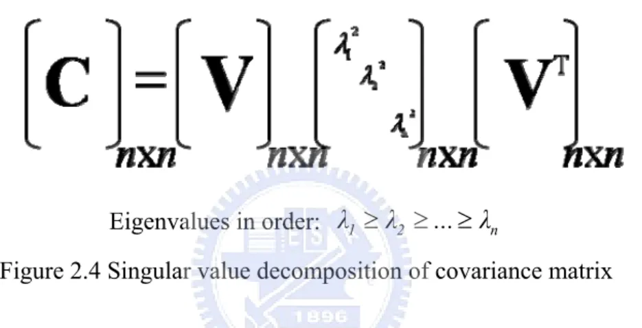
PCA is a self-organizing learning rule through Karhunen-Loeve (K-L)

transformation mapping into feature space [10]. Adaptive eigenvectors which were chosen construct subspace of the space. And data reconstruction is also using K-L transformation mapping into the subspace.

Given a set of data with dimension n and mean vector . We can compute the covariance matrix . Through singular value decomposition (SVD) processing as follows:

X m=E[X]=0 ] [_XT_X C = E Eigenvalues in order: λ₁ ≥λ₂ ≥...≥λ_n

Figure 2.4 Singular value decomposition of covariance matrix

Final, selecting the p (p≦n) largest eigenvalues corresponding eigenvectors construct matrix and discarding other eigenvectors in data representation. In regression, we shall add the LS phase after K-L transformation to estimate the curve fit. The regressive procedure is representable as:

∗

V

X∧ = XV∗ (2-6) Using LS method can acquire the weights.

_{∧ ∧} ∧ = X X Y X B _T T (2-7) - 7 -

Lease squares K-L transformation 1

x

∑

∑

y

2

x

x

_n ∗ 11

v

v

₁₂∗ ∗ 1a

v

...

1

x

∧1

x

∧

x

2 ∧ 2

x

∧

x

p ∧ p

x

∧ ∗ np

v

...

1

b

b

₂

b

_n

Figure 2.5 Three layer PCA architecture

2.3. Partial Least Squares (PLS)

PLS is one of the most general analysis methods in regression. Here we will

show PLS mathematic decomposition, regression algorithm and architecture of three layer multivariate system.

The independent variable matrix decomposed into matrix with corresponding weighting matrix and dependent variable matrix can be decomposed into matrix with corresponding weighting matrix . The mathematic form is represented as follows:

nxm X U_nxa 1 nx Y 1 ax Q mxa P nxa V ( ) ( ) ( ) T x x T T 2 2 T 1 1 2 1 x m a a n a a a m n

E

p

u

p

u

p

u

E

P

U

X

X

X

X

=

+

+

+

=

+

+

+

+

=

∧ ∧ ∧ ∧ ∧ ∧

L

L

E

+

_(2-8) ( ) ( ) ( ) 1 x x 2 2 1 1 2 1 1 a a n a a a nx

F

q

v

q

v

q

v

F

Q

V

Y

Y

Y

Y

=

+

+

+

+

=

+

+

+

+

=

∧ ∧ ∧ ∧ ∧ ∧

L

L

F

+

(2-9) - 8 -

Figure 2.6 PLS algorithm flow chart

After derivative, we exactly find out the residual matrix E_nxm and F_nx1 are minimized through the course of decomposing the matrix and .When computational iteration equation to a (a≦n) or the residual small than a minimum, PLS would terminate.

X Y

Ham [18] and Hsiao [9] bring up an idea which regards PLS as one kind of artificial neural networks. In the purpose, transformation between independent and dependent variables can be represented as three layer network architecture.

Figure 2.7 Three layer PLS architecture

2.4. Orthogonal Least Squares (OLS)

In this section, we describe OLS structure in the application for radial basis

function networks (RBFN) to select adequate centers. This rational approach provides an efficient learning algorithm for fitting appropriate RBFN. Let be independent matrix and be dependent matrix then the transformation can be written as:

] ,..., [x₁ x_n = X T 1,..., ] [y y_n y= y= Pθ+E (2-10) where T 1,..., ] [p p_n =

P ,p_i =[φ( x_i−x_j )], (.)φ is Gaussian function, with 1≦i,j≦n

T 1,..., ] [θ θ_n = θ T 1,..., ] [e e_n E= To make sense of the procedure clearly, we show the computational processing can be represented as:

E

E

θ

y

+

=

+

=

WG

A

W

(

)

[

x

1

,x

2

,...,x

n

]

=

X

[

(

i j

)

]

i

x

x

p

=

φ

−

[

]

T n 2 1

,p

,...,p

p

=

P

_,

(.) φ(.)

_{: Gaussian mapping}

φ(.)

_{: Gaussian mapping}

φ(.)

_{: Gaussian mapping}

φ

_{: Gaussian mapping}

Q-R decomposition

WA

P

=

W: orthogonal matrix A : strict upper triangle

Least squares method

1 T T

)

(

− ∧

=

W

W

W

G

y

Calibration

∧ ∧ ∧ ∧

=

=

=

≈

y

θ

θ

y

W

G

WA

P

Figure 2.8 OLS based on RBFN flow chart

Simplifying the OLS computational flow, we replace Q-R decomposition with orthogonal processing. Orthogonal decomposition of P can be obtained using Gram-Schmidt orthogonal processing computes a column of and selects an adequate regressor vector at a time. OLS makes a criterion to select the regressor vector and minimize the residual each iteration. The error criterion can be written:

A i

w

∑

(2-11) = + = n i i i iw w E E g y y 1 T T 2 T

Normalize (2-13) then we can acquire

w

_i due to error ratio (2-12)

output desired n calibratio y y E E y y y y w w g n i i i i = − =

∑

= T T T T 1 T 2 (2-12) According to (2-14), OLS can pick out an appropriate regressor vector with the error ratio mostly approximates to one each iteration.

i

w

Weights G between hidden and output layer

Hidden layer W

Symbol representation

Using LS method calculate weights Gram-Schmidt Orthogonal processing

Calculation process

1

x

x

₂

x

_n 11

g

∑

y

11

g

∑

∑

y

n

p

n

p

1

p

1

p

p

p

22 1

w

₁

w

1 − 11

a

−1 21

a

−1 n1

a

...

...

...

Gaussian mapping Regard as one layer

Figure 2.9 Three layer OLS architecture

There is no transformation mapping during Gram-Schmidt orthogonal processing so we shall regard two computational phases in front as one layer in Figure 2.9.

2.5. Regularization

Regularization techniques have been used in the past to avoid overfit [12], [16]

and error function of residual is minimized which depends on the network weights as well as the fit error [15]. Essentially it involves adding some multiple of a positive definite matrix to an ill-conditioned matrix so that the sum is no longer ill-conditioned and is equivalent to simple weight-decay in gradient descent methods.

Let’s define symbols to illustrate, and are two positive functions of , so we can try to determine by either

0 ] [u > A

u

0 ] [u > B

u

Minimize: A[u] or B[u] (2-13) In summary, regularization is Lagrange multiplier equation combines with quadratic constraint to minimize the weighted sum A[u]+λB[u] and lead to a adequate solution for . u

2.6. Regularized Orthogonal Least Squares (ROLS)

ROLS algorithm combines the advantages of both the orthogonal regression and

regularization methods to provide an efficient and powerful procedure for constructing models [12].

As mentioned earlier, the error criterion used in deriving the OLS algorithm is the total squared error . But the criterion in certain circumstances is prone to overfitting. To prevent overfitting, regularization method can be applied. Using (2-11), we define the residual squares error over the training set is

E

E

T

∑

= − = n i i i i D y y g w w E 1 T 2 T _(2-14)

And regularized term

∑

= = n i i R g E 1 2 _(2-15)

According to the regularization technique, it can be shown that the regularized error criterion can be expressed as

∑

∑

= = + − = + = n i i n i i i i R D e E E y y g w w g E 1 2 1 T 2 T _λ λ , with λ≥0. (2-16) Minimizing the equation

E

_e, we can get the appropriate term w_i.

Finally, we will show diagram of ROLS architecture to understand which computational phase is modified in Figure 2.10.

n p 1 p p2 1 x x₂ x_n 1

w

1

a

− 11 1

a

− 21 1

a

− n1 11

g

∑

y

...

...

...

n p 1 p p2 1 x x₂ x_n 1

w

1

a

− 11 1

a

− 21 1

a

− n1 11

g

∑

y

n p 1 p p2 1 x x₂ x_n 1

w

n pn p 1 p1 p pp22 1 x x₂ x_n 1

w

₁

w

1

a

− 11 1

a

− 21 1

a

− n1 11

g

∑

∑

y

...

...

...

Weights G between hidden and output layer

Hidden layer W

Gram-Schmidt Orthogonal

processing

Symbol representation

Calculate process

LS method Regularized techniques

combination

+

LS method Regularized techniques

combination

+

Gaussian mapping Regard as one layer Figure 2.10 Three layer ROLS architecture

Chapter 3. A novel method - Partial Regularized Least

Squares (PRLS

)

3.1. Relation between PLS and regularization

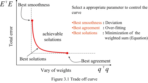
In this chapter, we will modify PLS architecture to reconstruct a novel calibration method, named as PRLS, to avoid overfitting which occurs when there is noise in the training data and the calibration system is flexible enough to fit to it. Here using the same symbols in section 2.3.

Original PLS calibrates during the processing of decomposing independent and dependent matrix, we only minimized the residual matrix E_nxm and F_nx1 . In the ideal situation, the calibration will approximate the desired output as minimum as it can be. But real data always goes along with hidden information that we have no idea whether it will interference the prediction or not. In this circumstance, PLS calibration may fit the noisy data and the outcome will lapse from our desire. We shall use the property of regularization and apply it to original architecture to solve this problem. As mentioned earlier, we exploit the concept of regularization techniques and rewrite the error criterion of PLS as:

E_e=E_D+λE_{R =}ETE_+λqTq, _{λ≥0 (3-1)} Where is weighting vector which inferences the output directly. In order to interpret equation and regularized parameter

q

e

E λ , we will illustrate using trade off curve as below

Total error

E

E

T

q

q

T Vary of weights

Best solutions _{Best agreement}

Best smoothness _{Select a appropriate parameter to control the}

curve

•Best smoothness: Deviation

•Best agreement : Over-fitting

•Best solutions : Minimization of the weighted sum (Equation)

achievable solutions

Figure 3.1 Trade off curve

Figure 3.1 illustrates that all achievable solutions are above the trade off curve but some of them conform our desire. Original PLS calibration reduces the total error as far as possible but if there is noise in training data, prediction may also fit the noisy data. Vary of weighting coefficients controls the curve motion and we add the term multiplies regularized parameter

q qT

λ to error criterion to make the calibration curve smooth without oscillating. In conclusion, PRLS keeps the calibration’s balance between smoothness of curve and accuracy.

3.2. PRLS algorithm

In the following, we will describe the modeling algorithm. Figure 3.2 points out the modulation to PLS. Although there are two computational phases using partial LS method, we only modify the later half because only the second half among two computational phases affects the executed output directly. Next, to understand the architecture obviously, we regard PRLS as a three layer neural network in Figure 3.3.

Figure 3.2 PRLS algorithm flow chart

Figure 3.3 Three layer PRLS architecture

Chapter 4. Experiments and discussion

This chapter will demonstrate our simulation experiment results including

simulation data and real data from 1D to 2D data and sound files. In the simulation data experiments, results show that PRLS has better performance than PLS and keep calibration stable with noise data. In the real data experiments, we apply our method to analyze environment sound measurement [19] and spectrum of blood glucose measurement [20].

4.1. Illustration

4.1.1.Synthesized simulation data

In simulation data calculation, we use synthesize three kinds of testing data with

noise to examine the efficiency of PRLS method. We add the noise generated by Gaussian probability density function with zero mean and set the value of standard deviation, so as to alter the level of noise. The noise to signal (N/S) ratio is also used to set up a standard of the variation. Given a signal data set and Gaussian noise data set with zero mean,

i

signal

i

noise 1≤i≤n. The mean of signal and noise data set are: n signal μ₌

∑

∀n i n noise μ n i N

∑

∀ = (4-1) The variance of a signal and noise data set are

n μ signal signal Var n i

∑

∀ − = 2 ) ( ) ( n μ noise noise Var n N i

∑

∀ − = 2 ) ( ) ( (4-2) The noise to signal (N/S) ratio is

) ( ) ( ratio signal Var noise Var S N _{= (4-3)} - 18 -

4.1.2. Criterion of estimation

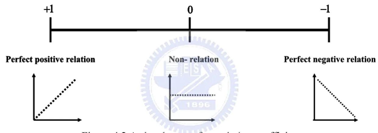
Two kinds of familiar standards are used to verify the performance of PRLS. It is also used to show the improvement of PLS when calibrating training data with outlier, prediction may overfit to noise. One of them is correlation coefficient indicates the strength and direction of a linear relationship between two variables. It refers to the departure of two variables from independence. The other is root mean square error (RMSE). RMSE is one of many ways to quantify the amount by which an estimator differs from the true value of the quantity being estimated like as a loss function. Following, we will illustrate with simple graphs.

Perfect positive relation Non- relation Perfect negative relation

+1 0 −1

Perfect positive relation

Perfect positive relation Non- relation Perfect negative relation

+1 0 −1 +1 0 −1

Figure 4.2 A sketch map of correlation coefficient

Several data sets of (x,y) points, with the correlation coefficient of x and y for each set. More approaching positive one more keeping consistency of direction between variables and distributing linearly. On the contrary, closing negative one indicates that the direction is opposite but distribution is also linear.

i

y

∧

Desired output

Prediction

i

x

i

y

X

Y

i i

y

y

∧

−

i

y

∧

Desired output

Desired output

Prediction

i

x

i

y

X

Y

i i

y

y

∧

−

n

y

y

n 1 i i i

∑

⎜

_⎝

⎛

−

⎟

_⎠

⎞

=

= ∧ 2

RMSE

Figure 4.3 Root mean square error

Figure 4.3 shows that the main concept of RMSE is to calculate the average of the distance between prediction and desired output data. To acquire accurate prediction, we hope that RMSE minimizes as far as possible.

4.1.2. Conditional training

Here we also calibrate the training data in different conditions — (1)

self-calibration & self-prediction (SCSP) and (2) cross validation (CV). In order to understand easily what is difference between SCSP and CV. We use diagrams to illustrate. Figure 4.4 shows the principle of SCSP and Figure 4.5 shows CV.

SCSP is a traditional training mode and the training data set is also prediction data set. Usually the result of SCSP is ideal if there is no noise hidden in the source data. However data usually goes along with noise and SCSP would be influenced by hidden information so that results may not necessarily meet to desire.

CV is also called leave one out (LOO) method because we select a validation data from original training data set and repeat until each observation in the set is used as validation data. The method also has the property of avoiding overfitting but costs heavy computation. Next, we will compare regularization technique and CV in simulation and real data experiments.

Prediction set

Calibration set

Calibrating

Predicting

The same set

Algorithm

Prediction set

Calibration set

Calibrating

Predicting

The same set

Algorithm

Figure 4.4 Self-calibration & self-prediction (SCSP)

Prediction set

Calibration set

Calibrating Predicting

Kept out

Returned

Algorithm

Prediction set

Calibration set

Calibrating Predicting

Kept out

Returned

Algorithm

Figure 4.5 Cross validation (CV)

4.2. Simulation data

In this section, PRLS and PLS will calibrate sigmoid and polynomial function

and imitative spectrum data under SCSP and CV. After predicting, we apply the criterion of estimation to examine which one is better among two methods and a brief discussion would be written down after experiments.

4.2.1. Sigmoid function

PRLS and PLS are used to approximate to the sigmoid function.

f(xi) = cos(xi), 0≦x≦2π (4-4)

One hundred training data were generated from f(xi)+εi, where xi has take from the

uniform distribution in (0,2π) and the noise ε had a Gaussian distribution with zero mean. The training data and the sigmoid function f(xi) are plotted in Figure 4.6. The

training data is highly ill-conditioned. Figure 4.7 depicts the correlation coefficient as a function of noise to signal ratio under SCSP and Figure 4.8 depicts the RMSE as a function of noise to signal ratio under SCSP. Figure 4.9 shows the network mapping constructed by PRLS and PLS algorithm with noise to signal ratio is 0.55.

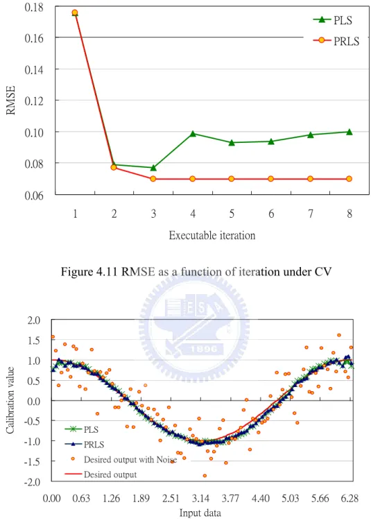
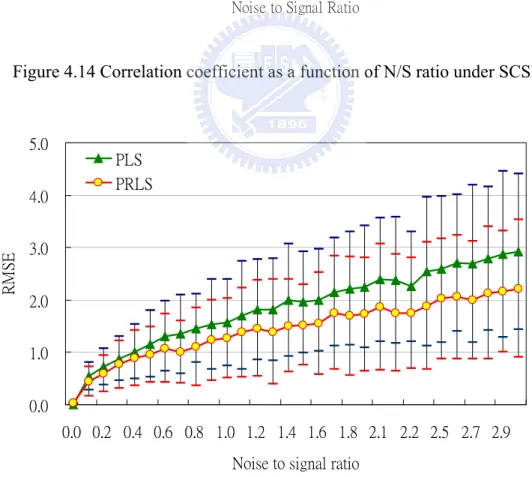
Under CV condition, we set N/S ratio = 0.55 and calibrate sigmoid function again. Figure 4.10 depicts correlation coefficient as a function of iteration. Figure 4.11 depicts RMSE as a function of iteration. Figure 4.12 shows that network mapping constructed by PRLS and PLS with noise to signal ratio is 0.55 under CV.

-2.0 -1.0 0.0 1.0 2.0 0.00 0.63 1.26 1.89 2.51 3.14 3.77 4.40 5.03 5.66 6.28 Input data x f( X ) Figure 4.6 Noisy training data (points) and sigmoid function (curve) with N/S ratio

= 0.55

0.40 0.50 0.60 0.70 0.80 0.90 1.00 0.00 0.28 0.55 0.85 1.13 1.41 1.69 1.94 2.18 2.56 Noise to Signal Ratio

C orr el atio n C oe ff ic ien t PLS PRLS

Figure 4.7 Correlation coefficient as a function of N/S ratio under SCSP

0.00 0.20 0.40 0.60 0.80 0.00 0.28 0.55 0.85 1.13 1.41 1.69 1.94 2.18 2.56

Noise to Signal Ratio

RM

S

E

PLS PRLS

Figure 4.8 RMSE as a function of N/S ratio under SCSP

-2.0 -1.0 0.0 1.0 2.0 0.00 0.63 1.26 1.89 2.51 3.14 3.77 4.40 5.03 5.66 6.28 Input data C ali br atio n va lu e PLS PRLS

Desired output with Noise Desired output

Figure 4.9 Network mapping constructed by PRLS and PLS algorithm under

SCSP with N/S ratio = 0.55 0.970 0.975 0.980 0.985 0.990 0.995 1.000 1 2 3 4 5 6 7 8 Executable iteration Cor rela tion coeff icient PLS PRLS

Figure 4.10 Correlation coefficient as a function of iteration under CV

0.06 0.08 0.10 0.12 0.14 0.16 0.18 1 2 3 4 5 6 7 8 Executable iteration RM SE PLS PRLS

Figure 4.11 RMSE as a function of iteration under CV

-2.0 -1.5 -1.0 -0.5 0.0 0.5 1.0 1.5 2.0 0.00 0.63 1.26 1.89 2.51 3.14 3.77 4.40 5.03 5.66 6.28 Input data C al ib ra tio n va lu e PLS PRLS

Desired output with Noise Desired output

Figure 4.12 Network mapping constructed by PRLS and PLS algorithm under CV with N/S ratio = 0.55

Table 4.1 Optimal CV results for sigmoid function data

PLS PRLS Correlation coefficient 0.9963 0.9971

RMSE 0.0772 0.0694 Adequate iteration 3 3

The results shown in above diagrams and table clearly demonstrate that the PRLS algorithm has better generalization properties

4.2.2 Polynomial function

In this experiment, we use polynomial function to examine.

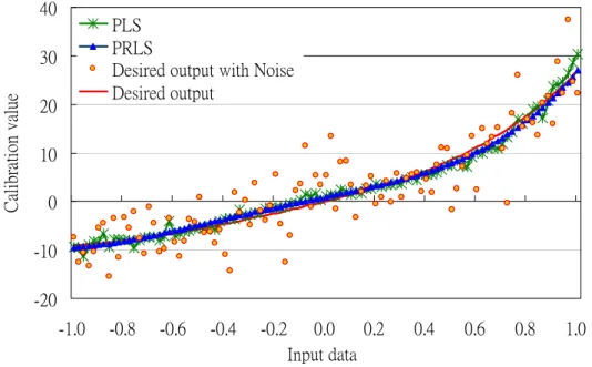
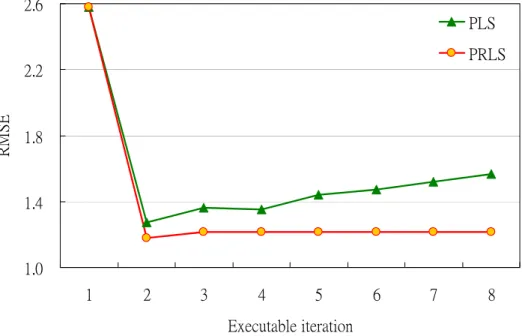
f(x) = 8th polynomial , -1≦x≦1 (4-5) We divide the range [-1,1] into one hundred parts and the training data were generated in the same way as 4.2.1. The noisy training data set and polynomial function were display in Figure 4.13. In the following, we will still estimate methods under SCSP and CV. Figure 4.14 depicts correlation coefficient as a function of noise to signal ratio and Figure 4.15 depicts RMSE as a function of noise to signal ratio under SCSP. PRLS and PLS prediction with noise to signal ratio is 0.55 under SCSP were plotted in Figure 4.16.

After examining under SCSP, we set constant noise to signal ratio to calibrate under CV and the records of correlation coefficient, RMSE and prediction were expressed in Figure 4.17, Figure 4.18 and Figure 4.19.

-20 -10 0 10 20 30 40 -1.0 -0.8 -0.6 -0.4 -0.2 0.0 0.2 0.4 0.6 0.8 1.0 Input data X f(X )

Figure 4.13 Noisy training data (points) and polynomial function (curve) with N/S

ratio = 0.55 0.2 0.4 0.6 0.8 1.0 0.00 0.20 0.40 0.61 0.80 1.03 1.19 1.44 1.65 1.84 2.07 2.22 2.47 2.70 2.88

Noise to Signal Ratio

C or rel at io n C oe ff ici en t PLS PRLS

Figure 4.14 Correlation coefficient as a function of N/S ratio under SCSP

0.0 1.0 2.0 3.0 4.0 5.0 0.0 0.2 0.4 0.6 0.8 1.0 1.2 1.4 1.6 1.8 2.1 2.2 2.5 2.7 2.9 Noise to signal ratio

RM

SE

PLS PRLS

Figure 4.15 RMSE as a function of N/S ratio under SCSP

-20 -10 0 10 20 30 40 -1.0 -0.8 -0.6 -0.4 -0.2 0.0 0.2 0.4 0.6 0.8 1.0 Input data Calibration value PLS PRLS

Desired output with Noise Desired output

Figure 4.16 Network mapping constructed by PRLS and PLS algorithm under SCSP with N/S ratio = 0.55 0.965 0.970 0.975 0.980 0.985 0.990 0.995 1.000 1 2 3 4 5 6 7 8 Executable iteration C or rel at io n co ef fi ci en t PLS PRLS

Figure 4.17 Correlation coefficient as a function of N/S ratio under CV

1.0 1.4 1.8 2.2 2.6 1 2 3 4 5 6 7 8 Executable iteration RM SE PLS PRLS

Figure 4.18 RMSE a function of N/S ratio under CV

-20 -10 0 10 20 30 40 -1.0 -0.8 -0.6 -0.4 -0.2 0.0 0.2 0.4 0.6 0.8 1.0 Input data Calibratio n valu e PLS PRLS

Desired output with Noise Desired output

Figure 4.19 Network mapping constructed by PRLS and PLS algorithm under CV with N/S ratio = 0.55

Table 4.2 Optimal CV results for polynomial prediction data

PLS PRLS

Correlation coefficient 0.9959 0.9967

RMSE 1.2738 1.1796 Adequate iteration 2 2

From experimental result, we can find out PRLS also has better performance than PLS whether the prediction is under SCSP or CV.

4.2.3 Imitative spectrum

We would like to generate two Gaussian functions g(x) with mean = 400 and

standard deviation = 20, h(x) with mean = 420 and standard deviation = 15. f(x) is the linear combination of g(x) and h(x) plotted in Figure 4.20.

0.00 0.01 0.02 0.03 0.04 0.05 380 390 400 410 420 430 440 450 460 470 480 Wavelength f( x) f(x) g(x) h(x)

Figure 4.20 Linear combination of two Gaussian functions with different mean and standard deviation

The training data set Xi +ε can be created by linear combination of g(x) and h(x)

with noise where x is the wavelength divided into one hundred identical parts. Desired output Y is the set of weighting coefficients. Figure 4.21 exhibits the training data. f(x)_i = Xi +ε= wi‧g(x) + (1/wi) ‧h(x) +ε, 1≦i≦10

Y= [w1,w2,…,w10] = [1,1.5,2,…,5.5] (4-6)

0.00 0.05 0.10 0.15 0.20 0.25 380 390 400 410 420 430 440 450 460 470 480 Wavelength f( x) f_01 f_02 f_03 f_04 f_05 f_06 f_07 f_08 f_09 f_10

Figure 4.21 Training data sets of imitative spectrum

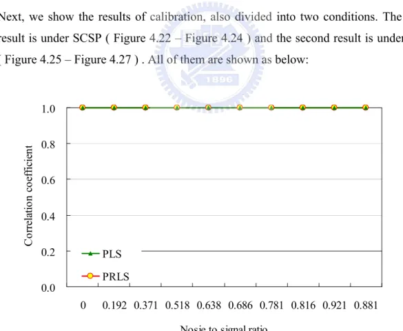
Next, we show the results of calibration, also divided into two conditions. The first result is under SCSP ( Figure 4.22 – Figure 4.24 ) and the second result is under CV ( Figure 4.25 – Figure 4.27 ) . All of them are shown as below:

0.0 0.2 0.4 0.6 0.8 1.0 0 0.192 0.371 0.518 0.638 0.686 0.781 0.816 0.921 0.881 Nosie to signal ratio

C or rel ati on co ef fi ci en t PLS PRLS

Figure 4.22 Correlation coefficient as a function of executable iteration under SCSP

0.0 0.2 0.4 0.6 0.8 1.0 0 0.192 0.371 0.518 0.638 0.686 0.781 0.816 0.921 0.881 Nosie to signal ratio

RM

S

E

PLS PRLS

Figure 4.23 RMSE as a function of executable iteration under SCSP

1.0 2.5 4.0 5.5

1 2 3 4 5 6 7 8 9 10

Spectrum data index

We ighting coefficie nt PLS PRLS Desired outptu

Figure 4.24 Network mapping constructed by PRLS and PLS algorithm under CV with N/S ratio = 0.55

0.980 0.985 0.990 0.995 1.000 1 2 3 4 5 6 7 8 9 Executable iteration Corr elation c oef fic ient PLS PRLS

Figure 4.25 Correlation coefficient as a function of executable iteration under CV

0.15 0.16 0.17 0.18 0.19 0.20 1 2 3 4 5 6 7 8 9 Executable iteration RM SE PLS PRLS

Figure 4.26 RMSE as a function of executable iteration under CV

1.0 2.0 3.0 4.0 5.0 6.0 1 2 3 4 5 6 7 8 9 10 Spectrum data index

W eighting Co efficients PLS PRLS Desired output

Figure 4.27 Network mapping constructed by PRLS and PLS algorithm under CV with N/S ratio = 0.55

Table 4.3 Optimal CV results for imitative spectrum prediction data

PLS PRLS Correlation coefficient 0.9980 0.9980

RMSE 0.1570 0.1520 Adequate iteration 2 2

4.2.4. Discussion

According to above diagrams and table, we can find out PRLS is improving and keeping prediction stable under noisy training data. Before applying our method to examine real data set, we have a brief discussion first.

Table 4.4 Compilation of simulated experimental results

Condition Criterion SCSP CV PRLS PLS PRLS PLS Correlation Coefficient RMSE Time

complexity

O(n)

O(n

2

₎

Condition Criterion SCSP CV PRLS PLS PRLS PLS Correlation Coefficient RMSE Time

complexity

O(n)

O(n

2

₎

N/S N/S N/S N/S Index Index Index Index

By observing results of simulation experiments, we made up table 4.4. Idealistically, we hope that result of prediction is high correlation coefficient, small RMSE and consumes light computation. Therefore we wish the height of correlation coefficient always keeps high and slop of RMSE is not abrupt and time complexity is as low as possible. From the table, we can clearly make out PRLS is advantageous among two methods in simulation data experiments.

4.3. Real data

4.3.1. Sound file

In the experiments, we would use ex-100 data to predict the 100th data with two

kinds of noisy sound files: (a) Power-station-ambience and (b) Transformer hum. We select 100 data sets to calibrate. Following, we would show the results of experiments. (a) Power-station ambience

Figure 4.28 Power station ambience source data

0.4 0.5 0.6 0.7 0.8 0.9 1 3 5 7 9 11 13 15 17 19 21 23 25 27 29 Index of hidden node

Correlation coefficien

Figure 4.29 Correlation coefficient as a function of index of hidden node under SCSP

Figure 4.30 RMSE as a function of index of hidden node under SCSP

t PLS PRLS 0.82 0.83 0.84 0.85 1 3 5 7 9 11 13 15 17 19 21 23 25 27 29 Index of hidden node

C or rel ati on co ef fi ci en t 0.030 0.031 0.032 0.033 0.034 0.035 1 3 5 7 9 11 13 15 17 19 21 23 25 27 29 Index of hidden node

RM S E PLS PRLS 0.030 0.035 0.040 0.045 0.050 0.055 1 3 5 7 9 11 13 15 17 19 21 23 25 27 29 Index of hidden node

RMSE

PLS PRLS

0.30 0.38 0.45 0.53 0.60 1 3 5 7 9 11 13 15 17 19 21 23 25 27 29 Index of hidden node

C orr el at io n co eff ici en t PLS PRLS

Figure 4.31 Correlation coefficient as a function of index of hidden node under CV

0.040 0.043 0.046 0.049 0.052 1 3 5 7 9 11 13 15 17 19 21 23 25 27 29 Executable iteration RMS E PLS PRLS

Figure 4.32 RMSE as a function of index of hidden node under CV Table 4.5 Optimal CV results for power station ambience prediction data

PLS PRLS Correlation coefficient 0.5646 0.5658

RMSE 0.0415 0.0411 Adequate iteration 6 6

(b) Transformer hum

Figure 4.33 Transformer hum source data

0.6 0.7 0.8 0.9 1.0 1 3 5 7 9 11 13 15 17 19 21 23 25 27 29 Index of hidden node

C or rel at io n co eff ici en t PLS PRLS

Figure 4.34 Correlation coefficient as a function of index of hidden node under SCSP

0.010 0.020 0.030 0.040 0.050 1 3 5 7 9 11 13 15 17 19 21 23 25 27 29 Index of hidden node

RM

S

E

PLS PRLS

Figure 4.35 RMSE as a function of index of hidden node under SCSP

0.30 0.43 0.55 0.68 0.80 1 3 5 7 9 11 13 15 17 19 21 23 25 27 29 Index of hidden node

C or rel at io n co eff ici en t PLS PRLS

Figure 4.36 Correlation coefficient as a function of index of hidden node under CV

0.0300 0.0350 0.0400 0.0450 0.0500 0.0550 1 3 5 7 9 11 13 15 17 19 21 23 25 27 29 Index of hidden node

RM

S

E

PLS PRLS

Figure 4.37 RMSE as a function of index of hidden node under CV Table 4.6 Optimal CV results for transformer hum prediction data

PLS PRLS Correlation coefficient 0.7490 0.7490

RMSE 0.0340 0.0330 Adequate iteration 6 6

4.3.2. Blood glucose data

Diabetes mellitus is one of the most common diseases in the present day, we can

analysis the blood glucose data and further control when the density is irregular. In the experiment, we select 37 data sets to evidence our purpose. Figure 4.28 shows blood glucose data with noise. In the following, we would show the results of calibration under SCSP and CV. Figure 4.29 shows that

-0.08 -0.04 0.00 0.04 0.08 900 975 1050 1125 1200 1275 1350 1430 1500 1580 Wavelength(nm) O. D

Figure 4.38 Blood glucose data with noise

0.4 0.5 0.6 0.7 0.8 0.9 1 1 5 9 13 17 21 25 29 33 37 Executable iteration C orre la tio n co effi ci en t 0.94 0.95 0.96 0.97 0.98 0.99 1.00 4 8 12 16 20 24 28 32 36 Executable iteration RM S E PLS PRLS PLS PRLS

Figure 4.39 Correlation coefficient as a function of executable iteration under SCSP

0 20 40 60 80 1 5 9 13 17 21 25 29 33 37 Executable iteration RM SE PLS PRLS

Figure 4.40 RMSE as a function of executable iteration under SCSP

0 50 100 150 200 250 300 350 400 1 5 9 13 17 21 25 29 33 37 Executable iteration Prediction PLS PRLS Desired output

Figure 4.41 Network mapping constructed by PRLS and PLS algorithm under SCSP

0.20 0.40 0.60 0.80 1.00 1 6 11 16 21 26 31 36 Executable iteration RM SE

Figure 4.42 Correlation coefficient as a function of executable iteration under CV

0.820 0.825 0.830 0.835 1 6 11 16 21 26 31 36 Executable iteration RM SE PLS PLS PRLS PRLS 40 50 60 70 80 90 1 6 11 16 21 26 31 36 Executable iteration RM SE PLS PRLS 41 41.5 42 42.5 43 1 5 9 13 17 21 25 29 33 Executable iteration RM S E PLS PRLS

Figure 4.43 RMSE as a function of executable iteration under CV

0 50 100 150 200 250 300 350 400 1 5 9 13 17 21 25 29 33 37 Executable iteration Prediction PLS PRLS Desired output

Figure 4.44 Network mapping constructed by PRLS and PLS algorithm under CV Table 4.7 Optimal CV results for blood glucose data

PLS PRLS Correlation coefficient 0.8240 0.8320

RMSE 42.280 40.993 Adequate iteration 6 7

4.3.3. Discussion

The same as the above section, we also draw a discussion. Due to the viewing

results of real experiments, we made up table 4.7 to show which one has better performance in real data experiments. We hope that result of prediction is high correlation coefficient, small RMSE and consumes light computation. Therefore we wish the height of correlation coefficient always keeps high and slop of RMSE is not abrupt and time complexity is as low as possible. From the table, we can clearly make out PRLS is advantageous among two methods in simulation data experiments.

Table 4.7 Compilation of real experimental results Condition Criterion SCSP CV PLS PRLS PLS PRLS Correlation Coefficient RMSE Time

complexity

O(n)

O(n

2

₎

Condition Criterion SCSP CV PLS PRLS PLS PRLS Correlation Coefficient RMSE Time

complexity

O(n)

O(n

2

₎

Index Index Index Index Index Index Index Index - 45 -

Chapter 5. Conclusion and future works

5.1. Conclusion

The purposed PRLS method is able to handle Gaussian noise under reasonable condition dataset. Although applying CV technique to calibration also has the same property. But we usually have no idea when prediction must terminate under CV in real data set. However our system can find out a value approximated to optimum in the end. Beside the time complexity of calculating under CV is O(N2), PRLS just consumes O(N). If we have a large amount of training data must calibrate, PLS is unsuitable.

From results of simulated experiments, the proposed scheme shows the robustness against the random noise generated by the Gaussian probability density function. In the real data experimental results, system also has better performance than original PLS method when calibrating training data with noise.

5.2. Future works

One of the most important properties of online system is that the response time must minimize as far as it can be. Therefore we consider to apply PRLS to online calibrated system. Although it would cost additional computational time, the amount is not worth mentioning. For the application of neural network, we can combine PRLS with backpropagation networks (BPN). PRLS can be used to initialize the weighting coefficients of BPN to keep BPN stable under noisy training data.

We only use linear transformation inside our scheme. In order to improve the efficiency of learning, developing the nonlinear model is necessary. For a high accuracy of calibration result, we can apply optimization algorithm to our purposed system to calculate the initial value of regularized parameter.

References:

[1] P. Bhandare, Y. Mendelson, R. A. Peura, G. Janatsch, J. D. Kruse-Jarres, R. Marbach, and H. M. Heise, Multivariate determination of glucose in whole blood using partial least-squares and artificial neural networks based on mid-infrared spectroscopy, Applied Spectroscopy, 47, 1214-1221, 1993.

[2] MÖCKS J., VERLEGER R., “Multivariate methods in biosignal analysis: application of principal component analysis to event-related”, Techniques in the behavioral and neural sciences, vol. 5, pp. 399-458 , 1991.

[3] Castellanos, G.; Delgado, E.; Daza, G.; Sanchez, L.G.; Suarez, J.F., “Feature Selection in Pathology Detection using Hybrid Multidimensional Analysis”, EMBS Annual International Conference, Aug 30-Sept 3, 2006.

[4] Oja, E., “A simplified neuron model as a principal component analyzer,” Journal of Mathematics and Biology, vol. 15, pp. 267-273, 1982.

[5] Harald martens and Tormod Naes, “Multivariate Calibration”, 2nd Edition, John Wiley & Sons, Great Britain, 1996.

[6] Kou-Yuan Huang, “Neural Networks and Pattern Recognition”, second edition,維 科圖書有限公司press, 2003

[7] C.-C. Chu, T.-C. Hsiao, C.-Y. Wang, J.-K. Lin, and H.-H Kenny Chiang, “Comparison of the performances of Linear Multivariate Analysis Method for Normal and Dyplasia Tissues Differentiation using Autofluorescence Spectroscopic”, IEEE Transactions of Biomedical Engineering, V. 53, No. 11, pp. 2265-2273, November 2006.

[8] Chih-Yu Wang, Tsuimin Tsai, Hsin-Ming Chen, Chin-Tin Chen, and Chun-Pin Chiang, "PLS-ANN Based Classification Model for Oral Submucous Fibrosis and Oral Carcinogenesis," Lasers in Surgery and Medicine, vol.32, no.4, pp. 318-326, 2003.04

[9] T.-C. Hsiao, C.-W. Lin, M.-T. Zeng, and H.-H. Kenny Chiang, “The Implementation of Partial Lease Squares with Artificial Neural Network Architecture”, IEEE-EMBS’98: 20th Annual International Conference of the IEEE Engineering in Medicine Biology Society, Honk Kong, China, October 1998. [10] Oja, E., and J. Karhunen, “Recursive construction of Karhunen-Loeve

expansions for pattern recognition purposes,” in Proceedings 5th Int. Conf. on

- 48 -

Pattern Recognition, Miami Beach, Fl., pp. 1215-1218 1980.

[11] Chen, S., C., F. N. Cowan, and P. M. Grant, “Orthogonal least squares learning algorithm for radial basis function networks,” IEEE Transactions on Neural Networks, vol. 2, pp. 302-309, 1991.

[12] Chen, S., Chng, E. S. And Alkadhimi, K. , “Regularized orthogonal least squares algorithm for constructing radial basis function networks”, international Journal of Control, 64:5, 829-837, 1996.

[13] Steve Lawrence, C. Lee Giles, Ah Chung Tsoi, “Lessons in neural network training: Overfitting may be harder than expected”, 14th national conference on artificial intelligence, pp.540-545, 1997.

[14] Fakultat fur Informatik, Universitat Karlsruhe, Karlsruhe, Germany, “Automatic early stopping using cross validation: quantifying the criteria”, Neural Networks 11, 761–767, 1998.

[15] Orr, M. J. L. , “Regularised centre recruitment in radial basis function networks,” Research Report, No. 59, Centre for Cognitive Science, University of Edinburgh, U.K. ,1993.

[16] MacKay, D. J. C. , “Bayesian interpolation,” Neural Computation, 4, 415-447, 1992.

[17] W. H. Press, S. A. Teukolsky, W. T. Vetterling and B. P. Flannery, "Numerical Recipes in C: The Art of Scientific Computing", 2nd Edition, Cambridge Univ. Press, 1994.

[18] F.M. Ham and I. Kostanic, “A Neural Network Architecture for Partial Least Squares Regression with Supervised Adaptive Modular Hebbian Learning”, Neural, Parallel, Scientific Computation, vol. 6, pp. 35-72, 1998.

[19] Jiun-Hung Lin, Pei-Chun Li, Shih-Tsang Tang, Ping-Ting Liu, and Shuenn-Tsong Young, “Industrial wideband noise reduction for hearing aids using a headset with adaptive-feedback active noise cancellation,” Medical & Biological Engineering & Computing. Volume 43, Issue 6, pp. 739-745, November, 2005. [20] T.-C. Hsiao, M.-T. Tseng, C.-W. Lin, G.-S. Hung, S.-W. Huang, and H.-H.

Kenny Chiang, “Near-infrared spectroscopic analysis of glucose concentration in aqueous and whole blood matrices”, Biomedical Engineering: Applications, Basis and Communications, 12, 195-204, August 2000.