基於分工報酬遞增的長期經濟發展：一項理論與實證分析

基於分工報酬遞增的長期經濟發展：一項理論與實證分析

研究成果報告(精簡版)

計 畫 類 別 ： 個別型

計 畫 編 號 ： NSC 95-2415-H-002-037-

執 行 期 間 ： 95 年 08 月 01 日至 96 年 09 月 21 日

執 行 單 位 ： 國立臺灣大學經濟學系暨研究所

計 畫 主 持 人 ： 孫廣振

計畫參與人員： 此計畫無參與人員：無

報 告 附 件 ： 國外研究心得報告

處 理 方 式 ： 本計畫可公開查詢

中 華 民 國 96 年 12 月 10 日

The Division of Labor, Capital, Communication

Technology and Economic Growth: The Case of

China 1952–99

Paresh Kumar Narayan and Guang-Zhen Sun*

Abstract

The implications of the division of labor, capital, and technology for economic growth have long been a fun-damental issue in development economics. This paper employs the bounds testing approach to cointegra-tion to examine the relacointegra-tionship between the division of labor, capital accumulacointegra-tion, communicacointegra-tion technology, and economic growth for China over the period 1952–99. We find that in the long run, capital stock and the division of labor both have statistically significant positive effects on growth, while in the short run the effects are not significantly positive. Telecommunication technology, rather surprisingly, has a sta-tistically insignificant impact on growth both in the long run and in the short run. Our findings indicate that there exists a long run equilibrium relationship between capital and the division of labor on the one hand, and economic growth on the other, thereby lending support to the division of labor theory of growth.

1. Introduction

For the two decades up to the Asian financial crisis in 1997, economic growth in China was 9.5% per annum, and after the Asian financial crisis it was about 7% per annum. Such economic performance over more than two decades can only be described as out-standing, and of significance to the world market given the size and the extent of open-ness of China’s economy. Naturally there has emerged a large body of studies examining the Chinese growth phenomenon, among which two recent analyses promi-nently focus on the extent of the Chinese domestic market. Young (2000) argues that during the post-Mao reform China’s government control of factor allocation has been moved from the central government to the provincial government level, resulting in increasing interregional government competition but at the price of fragmentation of the country-wide market, and the net effect is nonetheless growth of the market and welfare improvement. Keller and Shiue (2007) take a much longer perspective, con-sidering the behavior of the rice prices in the rice-producing provinces of central and southern China during the eighteenth to twentieth centuries, and find strong evidence of correlation between market integration and per capita income. In this paper, we also examine China’s growth from a long perspective, but focus on the economic history of the new China during the second half of the twentieth century. The novelty of our study of the Chinese economy is that it is informed by the division of labor theory of DOI:10.1111/j.1467-9361.2007.00393.x

* Narayan: School of Accounting, Economics and Finance, Faculty of Business and Law, Deakin University, Burwood, Vic. 3125, Australia. E-mail: [email protected]. Sun: Department of Economics, Monash University, Clayton, Vic. 3800, Australia. Tel: 61-3-9905-2409; Fax: 61-3-9905-5476; E-mail: [email protected]. We thank Peter Dixon, Yuxin Zheng, seminar participants at the Insti-tute for Quantitative and Technical Economics, the Chinese Academy of Social Sciences, and especially Elias Dinopoulos and two anonymous referees for their insightful comments, which considerably improved this paper. Sun’s research was supported by the (BusEco) Faculty Research Grant at Monash University as well as by the National Science Council of the Repulic of China (Taiwan) during his visiting professorship at the Department of Economics at National Taiwan University in 2006–2007. Any errors are our own.

economic growth and that for the first time in the time series economic growth liter-ature we explore the relationship between growth and division of labor. The study of the growth and division of labor nexus is important, for it has long been understood in economics, often referred to as the Smith Theorem, that economic growth is pro-foundly promoted by the division of labor, and that the division of labor is limited by the extent of the market (Smith, 1776; Stigler, 1951; for a recent empirical study sup-porting the importance of the extent of the market for economic growth, see Ades and Glaeser, 1999). What is relatively less understood, however, is that the extent of the market is also dependent on the division of labor, for the latter largely determines pro-ductivity and hence the “buying power” of the individuals in the economy at large (Young, 1928, pp. 539–40; for a recent formulation and elaboration of Young’s thesis on the interdependence between the extent of the market and the division of labor among other things, see Sun and Lio, 2003).1_{It is thus only natural to see the division}

of labor and the extent of the market as two sides of the same coin. Two factors that exert a decisive influence on the division of labor (and the extent of the market), long ago articulated by Smith as well, are the transport (transaction) condition in which the improvement enlarges the market size and engenders a finer division of labor, and capital, which serves as a vehicle for promoting the division of labor, especially in the manufacturing sector at Smith’s time. Among factors that contribute to improving the market transaction efficiency are postal and telecommunication facilities, which may well be used as a proxy for communication technology conducive to enlargement of the extent of the market. It goes without saying that capital, above and beyond facili-tating the division of labor, also directly makes a significant contribution to economic performance.

While the importance of capital accumulation and technology for economic growth have long been studied (Solow, 2001), it is only recently that there has emerged a lit-erature formulating the Smithian economics of the division of labor, and in particular, relating the division of labor to economic growth (e.g. Romer, 1987; Yang and Borland, 1991; Becker and Murphy, 1992; Sun and Lio, 2003; Yang, 2003). The central notion underlying this literature is increasing returns to the division of labor, which concep-tually differs from increasing returns to scale at the individual firm’s level as widely adopted in the textbooks, and is, therefore, deliberately referred to as generalized

increasing returns by Buchanan (1994) and macroeconomic increasing returns by

Currie (1997, prepared by Roger Sandilands). It is literally defined not as that based on the scale of operations of a particular firm or even a particular industry, but as that the production possibility frontier for the economy as a whole expands with the size of the nexus of exchanges and economic interdependence among its differing parts. Or in short, productivity and per capita income increase with the size of the network of the social division of labor. Enlargement of the network of division of labor allows for higher degrees of specialization, resulting in a higher productivity for the society as a whole, hence economic growth.2

Given the significance of the division of labor for economic growth, it would be of interest to systematically explore the determinants of the former. Several authors have argued in the last ten years that the principal determinants of the division of labor consist of far more elements than the Smithian transport condition.3_Knowledge,

trans-action institutions, uncertainty and insurance, information communication technology, and coordination costs each may also produce a profound influence on the division of labor and hence on economic progress (e.g. Becker and Murphy, 1992; Yang and Ng, 1993; Feeney, 1999; Sun and Lio, 2003). Each of the aforesaid elements consequently contributes to the economic growth via, but not always confined to, promoting

division of labor and hence promoting productivity. It is of both theoretical and policy interest to estimate empirically the contribution of these elements and explore their short-run vs long-run effects insofar as availability of data allows.

In this paper, we conduct an empirical study on the relationship between the divi-sion of labor, capital accumulation, communication technology, and economic growth for China over the period 1952–99. To achieve the aim of this study we use the bounds testing approach to cointegration, and find overwhelming evidence that GDP, the divi-sion of labor, capital stock, and the postal and telecommunication service facility are cointegrated and that the division of labor and capital stock both have statistically sig-nificant long-run effects on economic growth, while communication efficiency has a statistically weak effect on growth. Moreover, in the short run we find that capital stock, division of labour, and investment all contribute positively to growth, though the level of significance differs; however, telecommunication technology, as in the long run, has a statistically insignificant impact on growth. We also examine evidence for cointegra-tion between division of labour, capital, and communicacointegra-tion technology for two periods, 1952–99 and 1978–99, as dictated by available data, and find mixed evidence of a long-run relationship among these variables (details are found in subsection 3.3). To be sure, there have also been a few empirical analyses of the extent of the market and economic growth in addition to Young (2000) and Keller and Shiue (2007) as mentioned above. For instance, Yang et al. (1992) conducted detailed linear regression analyses of the institutional change in rural China during the period 1979–87 and exam-ined its implication for economic growth. They found that commercialization and institutional reform in specifying and enforcing property rights contributed sig-nificantly to economic growth. But the sample size of their data can hardly make their econometric analysis convincing. An interesting topic closely related to both the divi-sion of labor and economic growth is choice of techniques. In a study of the adoption of modern crop varieties in Punjab in India, McGuirk and Mundlak (1992) reported that the adoption of modern varieties is positively and significantly influenced by the density of roads. Ades and Glaeser (1999), using the conventional linear regression technique to analyze cross-country data on per capita GDP over the period 1960–85 and state-specific data on urbanization, transport facility, and labor force in the US over the period 1840–90, found that the division of labor is not only connected to urbanization but it is also important for economic development in general. In a recent empirical study on the division of labor and economic structural changes, Lio and Liu (2003) employed a cross-country dataset for 1996 to examine the (positive) effect of the transaction service facility on urbanization, which was therein used as a proxy for the division of labor. It should be noted that all these studies have used conven-tional linear regression analysis to test their hypotheses. This paper contributes to the literature by employing instead cointegration analysis, which is a superior method for spelling out the long-run and short-run relations between the division of labor, capital, communication technology, and economic growth, while conventional regression analyses cannot distinguish between long-run and short-run effects. To the best of our knowledge, our analysis is the first of its kind in the empirical literature to examine the relationship between extent of the market (division of labor) and economic growth.

The rest of the paper is organized as follows. We present our theoretical models and empirical strategy in the next section. In Section 3, we first describe in detail the data to be used, and then introduce the Dixit–Stiglitz index of the division of labor after carefully examining the instruments employed so far in the literature to measure specialization and regional-industrial concentration. After ascertaining the order of

integration by unit root tests, we conduct the error correction mechanism cointegra-tion analysis. The long-run and short-run relacointegra-tions between economic growth and explanatory variables including the extent of the market, the capital stock, net invest-ment, and postal and telecommunication facility are examined. Section 4 concludes.

2. Analytical Framework and Specifications

Two models are presented in this section. The first one is motivated by the theory that the division of labor, and capital accumulation and technology as well, contribute to economic growth. As mentioned earlier, increasing returns to the division of labor, through which the mechanism of how the economic performance in general and eco-nomic growth in particular are informed by the division of labor manifests itself, is dif-ferent from the concept of scale economies in some subtle yet crucial way. Each market participant’s choice of specialization in the network of exchange and social division of labor not only determines what and how much s/he demands from the market, but also informs the extent of market for other participants. By the same token, demand is dependent on the division of labor, but supply is largely determined by the extent of the market. In equilibrium, the productivity, and hence per capita income, of the society, is in great measure determined by the extent to which the labor is socially divided. Such a circular causality between the division of labor and the market volume would certainly be missed by looking only at the scale of operation of any particular firm or even any particular industry. Such a reciprocal demand approach to economic growth theory, which is largely attributed to the late Allyn Young in the literature (e.g., Sandilands, 2000) may have a similar ring to Sayian terms, but differs from Say’s Law in mechanism. It is therefore referred to, as indicated above already, as generalized increasing returns (Buchanan, 1994), the macroeconomic concept of increasing returns (Currie, 1997), the network effect of the division of labor (Yang, 2003; Lavezzi, 2003), etc., all of which are deliberately termed to emphasize the subtle yet fundamental dif-ference from the effect generated from scale of operation by particular individual pro-duction units. Indeed, Allyn Young has clearly drawn the distinction long before, “Large production, not large scale production, permits increasing returns” (1990, p. 54). We posit our first model informed by the division of labor theory of economic growth as follows:

(1a) where, as well as throughout the paper, per capita GDP is denoted by y, the proxy of the division of labor is denoted by D, per capita capital by k and communication facil-ity (technology) by T.4 _{Because capital is necessarily related to investment, further}

detail may be added to Equation (1a) to facilitate the empirical analyses below: (1b) where I stands for net investment per unit of labor and T for postal and telecommu-nication service facilities (as a proxy of the commutelecommu-nication efficiency).

The second model, which perhaps needs little conceptual explanation, describes the relation between the communication facility, capital, and the division of labor:

(2) Because capital stock enhances labor productivity, often remarkably, and communica-tion technology facilitates smoother market activities, both inform the extent of the market and the division of labor.

D=g k T

(

)

(

)

(

)

Taking models (1) and (2) together, both capital and the telecommunication facility contribute to economic growth not only directly by saving transportation and/ or telecommunication costs but also indirectly through promoting the division of labor.

Empirical Specifications

Based on our theoretical discussions above, we specify the following generic model to estimate the impact of division of labor, capital, and telecommunication technology on China’s GDP over the period 1952–99.

(3) Here, ln y is the natural log of per capita real GDP; ln k is the natural log of the capital–labor ratio, namely average capital stock per effective labourer; ln D is the natural log of the Dixit–Stiglitz index measuring the division of labor (a detailed expla-nation is found in the next section); ln I is the natural log of investment per labor; ln

T is the natural log of the postal and telecommunication service facilities, employed as

a proxy for telecommunication efficiency, and e is the error term. A priori, we expect that the division of labor and capital stock may positively impact China’s GDP. The impact of telecommunication efficiency is also expected to be positive.

Similarly, another theoretical model drawing on Equation (2) can be written in natural log form as follows:

(4) Here, all variables except the error term m are as defined previously.

3. Empirical Results

3.1. Data and Measurement of the Division of Labor

Since one major purpose of this article is to examine empirically the role played by the division of labor in economic performance over time, the period of our analysis is in great part dictated by availability of data from which we can construct the index measuring the division of labor. Leaving aside for the moment the detailed discussion of the measurement issues, we must first of all point out that our empirical analysis proceeds with two periods, 1952–99 and 1978–99, respectively, as informed by the fact that China’s statistics contain far more structural information about the social division of labor since the inception of the post-Mao reforms around 1978.

The series on real GDP is constructed by Hsueh and Li (1999) for the period 1952–95 and updated for the period 1996–99 from the China Statistical Yearbook 2004.5_Note

China starts its opening up and reform toward a market economy around 1979–80, and the national account system accordingly experienced a transformation from the mate-rial product balance (MPS) account, which was required for a planned economy but is seriously flawed for excluding the service sector, to a GDP system in the 1980s. With support from China’s National Statistical Bureau, appropriate adjustment of the data on GDP incorporating the added values from the service sectors has been made in Hsueh and Li (1999), which is regarded as more reliable than the official estimates of real GDP up to the 1990s (see, e.g., Bhalla et al., 2003, p. 28; Wang and Yao, 2003, p. 35). Admittedly, the notorious problem in dealing with the measurement of China’s output is not ideally solved by the two authors—perhaps it never can be solved

lnD=b₀+b₁lnk+b₂lnT+m.

entirely—Hsueh and Li (1999) nonetheless constitute a significant improvement in measuring the new China’s economic performance over about half a century since its establishment. Two particular contributions of Hsueh and Li (1999) may be high-lighted. First, they improved the deflators for output and investment for the period 1952–95 and recalculated the real output accordingly. Second, as mentioned above, they reconstructed the GDP data for the pre-reform China’s economy by making use of the historical data kept by the State Statistical Bureau to incorporate the service sector that is omitted in the MPS, thus making it comparable to the post-reform period. The annual data of country-wide population is taken from Comprehensive Statistical

Data and Materials on 50 Years of New China and updated from China’s Statistical Yearbook 2004. Population data of age 15–64 for period 1952–99 is from the

Appen-dix in Wang and Yao (2003).

The data on capital stock and investment for 1952–99 is also compiled by Wang and Yao (2003) and is available in an appendix to their article. The real capital stock series was constructed using the standard perpetual inventory approach. Data on post and telecommunication facilities, namely the number of post and telecommunication offices, is extracted from the Comprehensive Statistical Data and Materials on 50 Years

of New China and updated from China Statistical Yearbook 2004. The capital variable

conceptually encompasses both physical capital and human capital, yet due to the failure of the unit root test of human capital data (details available on request from the authors), this paper only employs the physical capital which is, of course, related to investment. Both institutions and technologies—technologies in transport and telecommunications in particular—may produce important influences on the extent of the market. This paper, however, considers only one important aspect of technologies, namely postal and telecommunication facility, largely due to the unavailability of reliable data, especially on institutions of sufficiently large size.6

Measurement of the division of labor is far more elusive than any of the aforemen-tioned variables. Theoretically, an axiomatic measure of the social division of labor is still embarrassingly lacking in the literature despite some interesting discussions. For instance, von Weizsäcker (1991), inspired by the Austrian capital theory, suggests a Shannon-entropy-like measure based on a matrix of the interpersonal benefits, a concept that remains to be well defined. In practice, quite a few indexes measuring the extent of the market as well as industrial or regional specialization have been employed in the literature. For instance, urbanization is used in both Ades and Glaeser (1999) and Lio and Liu (2003), as a proxy for the extent of the market in the former (p. 1041) and as a measure of the division of labor in the latter. In their study of the long-term economic development of China in the last three centuries, Keller and Shiue (2007) use the inverse of cross-province price variation to measure the integration (extent) of the market, and Zhou (2004) uses the real wage rate of the employee as a proxy of the extent of the market and the inverse of the number of goods being pro-duced as a measure of the specialization of the firm. As to measures of industrial and regional specialization, Dewhurst and McCann (2002) critically review 11 different measures, all having been used in the literature, among which the Herfindahl index measuring the industrial concentration, is of particular interest in understanding how labor is socially divided into different industries, for it at least reveals some structural information about the labor assignment in the society as a whole. But one crucial dif-ference between the concept of division of labor on the one hand and (regional) spe-cialization or industrial concentration on the other is that greater diversity of occupations and a more balanced distribution of labor allocation among different

sectors/industries imply a higher degree of the division of labor but a lower level of regional specialization or industrial concentration. The Herfindahl concentration index can be defined as H= , where eiis the employment share of industry/sector i.

Interestingly, a subtle but crucial modification of the Herfindahl index defined as such leads to what Ades and Glaeser (1999, pp. 1140–1) refer to as the Dixit–Stiglitz index for the division of labor, D= 2_{. It is easy to see that the Dixit–Stiglitz}

index describes both the variety of industries and the decentralization of the employ-ment among industries. For an economy like China over the period 1952–99 during which labor experienced a smooth but definitive shift roughly from the primary indus-try to the secondary and then the tertiary industries, this measurement appears to be a reasonable one. It is true that labor specialization of individuals is not measured by this measure. But in the case of China, the share of one’s production for exchange is far higher in the secondary and tertiary industries than in the primary one, and the employment structure among the three industries became more and more “balanced” during the nearly 50 years covered in this paper. What is behind the dramatic trans-formation is the enormous growth of products and services produced for exchange, namely, expansion of the market, and the deepening of the social division of labor.

On the other hand, admittedly, data availability can allow for only an imperfect measure of the change in division of labor for China during the period 1952–99. For the period 1952–78, only the data on employment structure among the three industries are available. Since 1978, data on employment share among 16 different sectors are available up to 2003. Unfortunately, reliable data on the real capital stock are not yet available for after 2000. As such, our empirical analysis below will proceed with two periods, namely the period 1952–99, based on the three-industry division of labor mea-surement, and the period 1978–99, based on the finer measurement of the 16-sector division of labor.

For the period 1952–99, data on percentages of employees in the primary, secondary, and tertiary industries (at the end of each year) are constructed, adjusted, and updated by reference to China’s Statistical Yearbook 2004 (p. 120), China’s Labor Statistical

Yearbook 1997 (p. 9), and the official website of the National Bureau of Statistics of

China: http://www.stats.gov.cn/. For the period 1978–99, we adopt data from China’s

Statistical Yearbook 2004 (p. 127) and China’s Labor Statistical Yearbook 1997

(pp. 10–11) to compute the employment share of the 16 sectors including: Farming, Forestry, Animal Husbandry and Fishery; Mining and Quarrying; Manufacturing; Elec-tricity, Gas and Water Production and Supply; Construction; Geological Prospecting and Water Conservancy; Transport, Storage and Communications; Wholesale and Retail Trade, Restaurants; Financial Intermediation and Insurance; Real Estate Activities; Social Services; Health Care, Sporting and Social Welfare; Education, Culture and Arts, Radio, Film and Television; Scientific Research and Polytechnic Ser-vices; Government Agencies, Party Agencies and Social Organizations; and others.

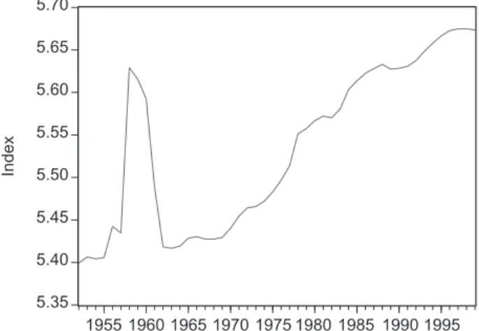
We plot the natural logarithm of the division of labor index, calculated using the two different datasets for these two periods in Figures 1 and 2.7_{It is worth mentioning the}

politico-economic background to the anomaly in the trend of the evolving division of labor that occured during 1958–61, the Great Leap Forward movement. Although Maoist China is characterized by political movements one after another which inces-santly left their marks in the economic history of the new China, the Great Leap Forward still stands as an exceptionally remarkable event in terms of profoundness of

ei i

∑

∑

its economic outcomes. Without delving into historical details (see, e.g., chapter 6 in Riskin 1987 for a political economy analysis of the background, nature, process, and consequences of the Great Leap Forward and the Utopianism part in Meisner 1999 for a wider perspective), we would like to point out that the dramatic change in employee percentage, especially sharp declining in the primary industry and increas-ing in the secondary industry, reflects the extraordinary changes in total number of employees in the non-agricultural industries resulting from the Great Leap Forward movement, which is essentially a consequence of the military approach to economic development led largely by Mao and his radicals and which turned out to be a huge failure with disastrous consequences. Table 1 may reveal some important information. In a similar vein, the collapse that occured in the social division of labor series around 1989 as shown in Figure 2, a far less sharp decline compared to the Great Leap Forward period, was rooted in the change in the employment structure among sectors

5.35 5.40 5.45 5.50 5.55 5.60 5.65 5.70 1955 1960 1965 1970 1975 1980 1985 1990 1995 Index Year

Figure 1. Division of Labor Index in Natural Log Form, 1952–99

6.32 6.36 6.40 6.44 6.48 6.52 6.56 6.60 1978 1980 1982 1984 1986 1988 1990 1992 1994 1996 1998 Index Year

caused by the austerity measures the government started taking in late 1988 to slow down the “overheated” macroeconomy. Resulting from the expansionary market poli-cies of 1987 and early 1988, the annual inflation rate in the autumn of 1988, at least in major cities, reached an alarming 30%, thus forcing the government to considerably tighten the credit and cut off the investment and money supply.8_{The tight control on}

credit resulted in the closure of many factories dependent on easy credit, among which “the particularly hit were the town and village enterprises (TVEs), the most dynamic sector of the Chinese economy, which had been increasing output at rates near to 30 percent per annum, which employed nearly 100,000,000 workers in the late 1980s” (Meisner, 1999, p. 492). Production declined and a lot of laid-off workers, especially from the TVEs, were forced to re-enter sectors in the primary industry in late 1989 and early 1990.9

3.2. Unit Root Tests

To ascertain the order of integration we apply the Augmented Dickey-Fuller (ADF; Dickey and Fuller, 1979, 1981) and Phillips and Perron (PP, 1988) unit root tests. While the bounds test for cointegration among several variables does not require a test for the presence of unit roots of individual series, application of the long-run estimators does require this exercise. To accomplish this, we use the ADF test based on the auxiliary regression:

(5) The ADF auxiliary regression tests for a unit root in xt, namely GDP, capital stock,

investment, and proxies for division of labor and telecommunication facility at time t;

t denotes the deterministic time trend;Δxt−i is the lagged first differences to

accom-modate serial correlation in the errors, mt; and a, d, b and y are the parameters to be

estimated. The null and the alternate hypotheses for a unit root in xtare:

While relevant critical values are available from various sources, we use the approxi-mate critical values compiled by MacKinnon (1991).

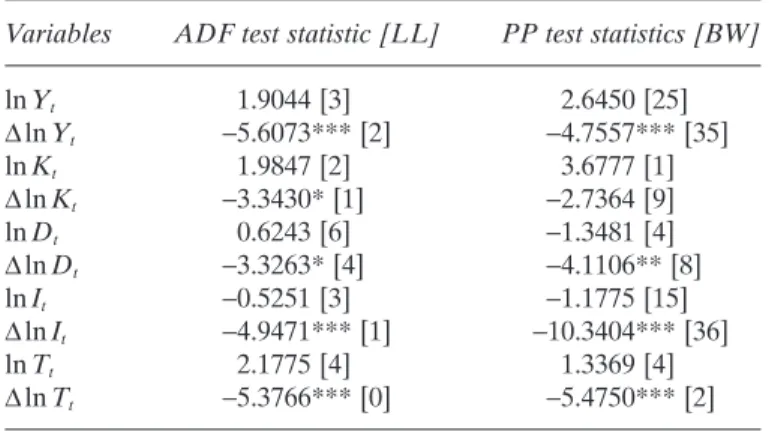
Table 2 reports the results of the unit root tests. The ADF statistic for the levels of GDP, capital stock, investment, and proxies for division of labor and communication

H0:b=0 H1:b<1. Δxt t xt iΔxt i t i k = + + − + − + =

∑

Table 1. Total Number of Employees in the Primary, Secondary and Tertiary Industries Around the Great Leap Forward Period (at the end of each year, in 10,000 persons)

Year Primary industry Secondary industry Tertiary industry

1957 19,309 2,142 2,320 1958 15,490 7,076 4,034 1959 16,271 5,402 4,500 1960 17,016 4,112 4,752 1961 19,747 2,856 2,987 1962 21,276 2,059 2,575

efficiency [y, k, D, I, T] do not exceed the critical values (in absolute terms). However, when we take the first difference of each of the variables, the ADF statistic is higher than the respective critical values (in absolute terms). Therefore, we conclude that [y, k, D, I, T] are each integrated of order one or I(1).

To ensure the robustness of the ADF test results, we also apply the PP test for unit roots. The PP test is also based on equation (5), but without the lagged differences. While the ADF test corrects for higher order serial correlation by adding lagged difference terms to the right-hand side, the PP test makes a non-parametric correction to account for residual serial correlation. Monte Carlo studies suggest that the PP test generally has greater power than the ADF test (see Banerjee et al., 1993, p. 113).

The PP test is also reported in Table 2 and the results are consistent with those from the ADF test. For instance, we find that the PP statistic does not exceed the critical values (in absolute terms) for the levels of [y, k, D, I, T]. However, when we take the first difference of each of the variables, the PP statistic is higher than the respective critical values (in absolute terms). Therefore, we conclude that [y, k, D, I, T] are each integrated of order one or I(1).10

3.3. Cointegration

To implement the bounds testing procedure, it is essential to model Equation (1) as a conditional autoregressive distributed lag model as follows:

(6) Δ Δ Δ Δ Δ Δ ln ln ln ln ln ln ln ln ln ln ln y y k D I T y k D I T t t t t t t i t i i p j t j l t l l p j p m t m n t n n p m = + + + + + + + + + + + − − − − − − = − − = = − − = =

∑

∑

∑

∑

∑

Table 2. Integration Properties of the Data

Variables ADF test statistic [LL] PP test statistics [BW]

ln Yt 1.9044 [3] 2.6450 [25] ΔlnYt −5.6073*** [2] −4.7557*** [35] ln Kt 1.9847 [2] 3.6777 [1] ΔlnKt −3.3430* [1] −2.7364 [9] ln Dt 0.6243 [6] −1.3481 [4] ΔlnDt −3.3263* [4] −4.1106** [8] ln It −0.5251 [3] −1.1775 [15] ΔlnIt −4.9471*** [1] −10.3404*** [36] ln Tt 2.1775 [4] 1.3369 [4] ΔlnTt −5.3766*** [0] −5.4750*** [2]

Notes: Critical values are generated using Monte Carlo simulations using 10,000 replications. The critical values are −4.2733, −3.5578, and −3.2124 at the 1 per cent, 5 per cent, and 10 per cent levels of significance, re-spectively. *, **, *** denote statistical significance at the 10%, 5%, and 1% levels, respectively. LL stands for lag length and BW stands for bandwidth.

Here, all the variables are as previously defined. The bounds test for examining evi-dence for a long-run relationship can be conducted using either the F-test or the t-test. The F-test tests the joint significance of the coefficients on the one period lagged levels of the variables in equation (6), that is, H0:q1= q2= q3= q4= q5= 0, while the t-test tests

the null hypothesis H0:q1= 0. The asymptotic distribution of critical values is obtained

for cases in which all regressors are purely I(1) as well as when the regressors are purely I(0) or mutually cointegrated.

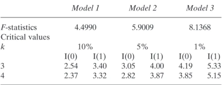
The asymptotic critical value bounds of the F-statistic, based on equation (6), for cointegration are reported in Table 3. Note we make use of approximate critical values of the bounds F-test for relatively small sample sizes, which are substantially different from critical values when there are very many observations as considered in Pesaran et al. (2001). See Appendix A in Narayan (2005) for a new set of critical values of the bounds F-test for sample sizes ranging from 30 to 80. For cointegration to exist, the value of the estimated statistic needs to be higher than the upper bound critical value. We consider three variants of equation (3). In model 1, we exclude the commu-nication technology variable, in model 2 we include commucommu-nication technology but exclude the investment variable, while in model 3 we include all the variables as in equation (3). For models 1 and 2, to test for cointegration we accordingly modify equa-tion (6). Across all models capital and division of labor are the common variables. From Table 3 it can be seen that the value of the calculated F-statistic is higher than the upper bound critical value for all the three models, implying that we are able to reject the null hypothesis of no cointegration. This leads us to the conclusion that there is cointegration between all the variables in each of the three models. This allows estimation of elasticities in the models wherein the natural log of each variable is employed.

We can similarly conduct the bounds test for cointegration based on equation (2). The F-statistic for the sample period 1952–99 turned out to be 0.9334, which is less than the 10% critical value; hence, we conclude that there is no long-run relationship between division of labor, physical capital, and telecommunication technology. However, when we conduct the cointegration test for the period 1978–99 where divi-sion of labor is calculated taking the 16 sector data, the calculated F-statistic turned out to be 4.0135 which is greater than the critical value at the 10% level, implying that we can reject the null of no cointegration. (We omit the details to save space here. Full results are available from the authors on request.) Despite this finding, we would like to exercise caution given the relatively small sample size for this model. For this reason, we will not conduct the elasticity analysis for equation (2) (and hence equation (4)) below.

Table 3. Bounds F-test for Cointegration Based on Equation (3) Model 1 Model 2 Model 3

F-statistics 4.4990 5.9009 8.1368

Critical values

k 10% 5% 1%

I(0) I(1) I(0) I(1) I(0) I(1)

3 2.54 3.40 3.05 4.00 4.19 5.33

4 2.37 3.32 2.82 3.87 3.85 5.15

3.4. Long-run and Short-run Elasticities

To estimate the long-run elasticities we use the Dynamic Ordinary Least Squares (DOLS) procedure advocated by Stock and Watson (1993) and the Fully Modified Ordinary Least Squares (FMOLS) procedure developed by Phillips and Hansen (1990). The DOLS involves estimation of long-run equilibria via dynamic ordinary least squares, which corrects for potential simultaneity bias among regressors. Per-forming the DOLS technique involves regressing one of the I(1) variables on other I(1) variables, the I(0) variables, and lags and leads of the first difference of the I(1) variables. The main advantage of incorporating the first difference variables and the associated lags and leads is to obviate simultaneity bias and small sample bias inher-ent among regressors. The DOLS is based on an alternative represinher-entation of the system which assumes the following particular a priori normalization that can be obtained in any system with r cointegrating vectors:

(7a) (7b) where , the dimensions of and being (p− r) × 1 and (r × 1), respec-tively. The error processes are deemed stationary and by incorporating both leads and lags of Δ in equation (7a) and estimating the normalized cointegrating vectors,Φ, by OLS, one can obtain an estimator asymptotically equivalent to the maximum like-lihood estimation.

Meanwhile, the FMOLS estimator has two important advantages. Apart from cor-recting for endogeneity and serial correlation effects it also asymptotically eliminates the sample bias. There are two conditions considered essential for the appropriateness of the FMOLS. First, there is only one integrating vector. Second, the explanatory vari-ables are not cointegrated among themselves. Assuming these provisions are met, the econometric model is of the following form:

(8) where ytis an I(1) variable and Xtis a (k× 1) vector of I(1) regressors, which are not

cointegrated among themselves. By assumption, Xthas the following first difference

stationary process:

(9) where h is a k× 1 vector of drift parameters, ltis a k× 1 vector of I(0) variables. It is

also assumed that vt= (mt, )′ is strictly stationary with zero mean and a finite

posi-tive-definite covariance matrix,Σ.

The Granger representation theorem states that in the presence of a cointegrating relationship among variables, a dynamic error correction representation of the data exists. Following Engle and Granger (1987) we estimated the following models to capture the short-run and the long-run adjustment to equilibrium relationships:

(10) Δ Δ Δ Δ Δ Δ ln ln ln ln ln ln y y k D I T t q t q q t q q t q q m q m q m q t q q t q t t q m q m = + + + + + + + − − − = = = − − − = =

∑

∑

∑

∑

∑

All variables in Equation (10) are as defined previously. mtand etare the disturbance

terms;Δ is the first difference operator; et−1 is the error correction term (one lagged

error) generated from equation (3), and m is the lag length. By specification, equation (10) consists of lagged dependent and independent variables, and a ‘test down’ proce-dure is employed repeatedly until the most parsimonious specification is achieved.

Equation (10) captures both the short-run and long-run adjustment to equilibrium relationships between per capita income and a set of explanatory variables. The adjust-ment to equilibrium relationship is captured by the lagged value of the long-run error correction term, expected to be negative, reflecting how the system converges to the long-run equilibrium implied by equation (3); convergence is assured when d is between 0 and −1.

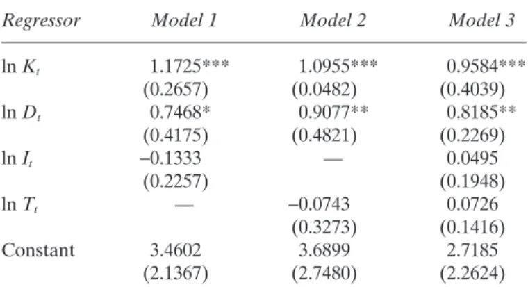
The long-run results for equation (3) are reported in Table 4. We report three ver-sions of equation (3) just to gauge the robustness of the results. As mentioned earlier, in model 1, we exclude the telecommunication efficiency variable, in model 2 we include telecommunication efficiency but exclude the investment variable, while in model 3 we include all the variables as in equation (3). Across all models capital and

Table 4. Long-run Elasticities Panel A: DOLS estimator

Regressor Model 1 Model 2 Model 3

ln Kt 1.1725*** 1.0955*** 0.9584*** (0.2657) (0.0482) (0.4039) ln Dt 0.7468* 0.9077** 0.8185** (0.4175) (0.4821) (0.2269) ln It −0.1333 — 0.0495 (0.2257) (0.1948) ln Tt — −0.0743 0.0726 (0.3273) (0.1416) Constant 3.4602 3.6899 2.7185 (2.1367) (2.7480) (2.2624)

Panel B: FMOLS estimator

Regressor Model 1 Model 2 Model 3

ln Kt 0.8557*** 0.9413*** 0.8557*** (0.1044) (0.0602) (0.1044) ln Dt 1.0114* 1.1021** 1.0114** (0.4622) (0.4698) (0.4762) ln It 0.2169 — 0.06901 (0.1443) (0.1044) ln Tt — 0.1037 0.2161 (0.1790) (0.1443) Constant 0.0506 0.6297 0.0506 (2.6469) (2.6170) (2.6469)

Note: standard errors are in parentheses. ***, **, * denote statistical significance at the 1%, 5%, and 10% levels, respectively.

division of labor are the common variables. Both the DOLS and the FMOLS estima-tors11_{reveal that capital stock and division of labor have a positive and statistically}

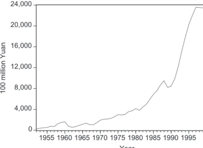
sig-nificant relationship with per capita income in the long run across all the three models. According to model 3, for instance, a 1% increase in capital stock increases growth by around 0.95%; and a 1% increase in division of labor increases growth by some 0.82%. Meanwhile, the coefficient on investment has a relatively small magnitude and while it has the expected sign, it is statistically insignificant in explaining per capita income. This result is not surprising when one examines the trend in real investment for China over the sample period 1952–99 (Figure 3). Real investment only accelerated follow-ing the reforms in 1978; hence, it is unlikely, given the relatively small sample size of post-reform data (22 years), that our long-run model captures the full impact of invest-ment on growth. Given this limitation of our sample size and the history of China’s investment performance, one should view our results on investment with caution, for our results do not imply that investment is not important for growth. In model 2 where we exclude investment but include communication efficiency, we find that while both capital and division of labor contribute positively and significantly (at the 1% and 5% levels, respectively) to growth, telecommunication efficiency has a statistically insignif-icant impact on growth. In model 3, where all variables are included, two results are worth noting. First, consistent with the results from models 1 and 2, we find capital and division of labor having a statistically significant and positive (at the 1% and 5% levels, respectively) impact on growth. Second, the impact of telecommunication efficiency and investment is at best statistically weak.12

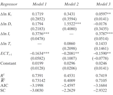
The short-run results are reported in Table 5.We find mixed results in terms of effects of capital and the division of labor on per capita income. In models 1 and 3 investment is statistically significant and positively contributes to per capita income, while only in model 2 is division of labor statistically significant and positive at the 1% level of sig-nificance in explaining per capita income. Capital’s contribution to growth is statisti-cally significant only in model 3, at the 5% level of significance. Moreover, according to the Akaike Information Criterion (AIC) and the Schwarz Criterion (SC), model 1 turns out to be the preferred model since both the AIC and SC are minimized for this model. Meanwhile, across all models we find that telecommunication facilities are sta-tistically insignificant in contributing to growth. More importantly, the error correction

0 4,000 8,000 12,000 16,000 20,000 24,000 1955 1960 1965 1970 1975 1980 1985 1990 1995 100 million Yuan Year

terms ECTt−1in the short-run models are all statistically significant at the 5% level or

better with a negative sign, confirming that a long-run equilibrium relationship exists between the variables, and the low magnitude of the coefficients reflects that adjust-ment to equilibrium is fairly slow.

4. Concluding Remarks

We conduct error correction mechanism analysis for cointegration to examine the relationship between the division of labor, capital, telecommunication technology, and economic growth in China for the period 1952–99. We find strong evidence of cointegration among these variables. We then employ the dynamic ordinary least squares and the fully modified ordinary least squares techniques to explore the long-run and the short-long-run relationships among the above-mentioned variables. We find that in the long run, capital stock and the division of labor both have statistically signifi-cant positive effects on economic growth, while in the short run their effects on growth are not significantly positive. Investment has a statistically significant positive impact on growth in the short run but not in the long run. Telecommunication technology, rather surprisingly but explicably (see below), has a statistically insignificant impact on growth both in the long run and in the short run. We also examine evidence for coin-tegration between division of labor, capital, and telecommunication technology and find no strong evidence of a long-run relationship among these variables. Thus our main finding is that there exists a long-run equilibrium relationship between capital, the division of labor on the one hand and economic growth on the other, thereby lending strong support to the division of labor theory of growth. To the best of our knowledge, our cointegration analysis is the first of its kind in empirical studies on the relationship between the division of labor and economic performance.

Table 5. Short-run Elasticities

Regressor Model 1 Model 2 Model 3

Δln Kt 0.1719 0.3431 0.0597** (0.2852) (0.3594) (0.0141) Δln Dt 0.1794 1.5522*** −0.0176 (0.2183) (0.4080) (0.3435) Δln It 0.3756*** — 0.3787*** (0.0478) (0.0514) Δln Tt — 0.0860 0.1433 (0.2098) (0.1461) ECTt−1 −0.1634*** −0.2081** −0.1590** (0.0582) (0.1007) (−0.0778) Constant 0.0199 0.0296 0.0246 (0.0128) (0.0206) (0.0141) R2 _{0.7391 0.4531 0.7419} 2 _{0.73142 0.4009 0.7105} AIC −3.1998 −2.4597 −3.1684 SC −3.0030 −2.2629 −2.9322

Note: t-statistics are in parentheses. ***, ** denote statistical significance at the 1% and 5% levels, respectively.

As already indicated in subsection 3.1, the time series data of human capital does not survive the unit root test and therefore we cannot make a long-run estimate of its contribution to economic growth. A few more words may be in order here. Because of the social and political movements during the late 1950s–late 1970s (especially the Cultural Revolution 1966–76), the education system in China experienced abrupt changes during this period. For instance, the higher education system virtually broke down and very few students with a bachelor’s degree were produced during the Cul-tural Revolution. This may well explain why human capital time series data fails the unit root test, and as a consequence we cannot include human capital into our cointe-gration analysis, although human capital may, just like physical capital, make a directly significant contribution to economic growth, as revealed in Wang and Yao (2003). In addition, we would speculate that human capital accumulation, which may be seen as a reasonably acceptable proxy for growth in knowledge, may also indirectly contribute to growth via promoting the division of labor as theoretically predicted (e.g. Becker and Murphy, 1992; Yang and Ng, 1993), should the human capital time series data otherwise survive the unit root test.

That capital significantly contributes to growth in the long-run equilibrium cannot be anything new to economists (e.g. Solow, 2001). As to the rather weak effect that the telecommunication technology has on economic growth, a finding that seems to be inconsistent with the extent of market theory of economic development as outlined earlier, it is necessary to emphasize that dramatic improvement in telecommunication technology in China occurred in the early to mid 1990s and it certainly takes time for the effect of such technology changes on the extent of the market to fully play out. Like telecommunication technology, investment also displays a weak relationship with per capita income in the long-run equilibrium. But this is not entirely surprising given that investment only started to perform after the reforms had intensified during the late 1980s onwards, implying that given the small sample size we were not able to fully capture the impact of investment. Hence, both the roles of telecommunication tech-nology and investment remain an issue to be revisited in future research. Our most important finding is that the long-run relationship between the division of labor and per capita income is positive and statistically significant, confirming the prediction by the division of labor theory of market process. As already explained in detail when dis-cussing the data and measurement problems in section 3, we can only use a rather imperfect measure of the division of labor, as dictated by both the available data and lack of a theoretically well founded measure of the social division of labor. Nonethe-less, this measure has proved illustrative in spelling out how the structure of employ-ment informs economic growth (e.g. Ades and Glaeser, 1999). The present study represents the first attempt to construct a time series division of labour index, which enables us to analyze the impact of the division of labor, together with other variables, on per capita income both in the long run and in the short run.

Although, theoretically speaking, the extent of the market and the division of labor are in a great measure interdependent, the interplay between them and the mecha-nism through which they inform economic development in reality can be considerably affected by other factors. As far as China’s economy is concerned, much work remains to be done in understanding the underpinning political economy of inter-regional divi-sion of labor in particular. Indeed, for a large developing economy like China, the domestic market plays a key role in shaping its economic landscape. In their study of the rice markets in central and southern China over last three centuries, Keller and Shiue (2007), considering the interregional price convergence as a proxy of market integration, find that the degree of market integration and trade in the 1720s–1730s

can well serve as a predictor of GDP per capita at the end of the twentieth century. This is an important finding, for it indicates the possibility that the short-run effect of the economic reform may be more or less exaggerated while the fundamental role played by the extent of the market in the long run is somehow overlooked, or at least understated. This observation not only lends support to Young’s criticism that the growing interregional barriers to trade and hence to interregional division of labor resulting from the incremental reform lead to a significant, yet often overlooked, loss in efficiency, but is also quite consistent with the division of labor theory of market process as outlined earlier. The present analysis focuses on the aggregate time series data over the period 1952–99 to investigate, rather preliminarily, the long-run impact of the division of labor on economic growth. It is worthwhile to further explore how the extent of the market and the division of labor inform economic growth by com-paring historical performance across regions. To be sure, neither integration of market, as measured by the interregional price convergence (Keller and Shiue, 2007) nor the urbanization rate (Ades and Glaeser, 1999; Lio and Liu, 2003), is the same thing as the extent of the market per se. A much more detailed analysis based on historical data is thus needed for quantitatively estimating the extent of the market for each region. The katallactic approach as advanced by the Austrians and James Buchanan may provide a useful device to measure the market volume (see, for instance, Cochran 2004 for a recent attempt to measure the extent of the US market over the period 1919–39 by looking at the volume of check clearings). Measurement of the division of labor may also need to be elaborated when coming to grips with economic structures at the regional level. We plan to devote more future research to expanding our analysis here by carefully constructing and closely examining the panel data of regional develop-ment in China over the second half of the twentieth century, as informed by the divi-sion of labor theory of market process.

References

Ades, Alberto F. and Edward L. Glaeser, “Evidence on Growth, Increasing Returns and the Extent of the Market,” Quarterly Journal of Economics 114 (1999):1025–45.

Banerjee, Anindya, Juan Dolado, J. W. Galbraith, and David Hendry, Cointegration, Error

Cor-rection and the Econometric Analysis of Non-Stationary Data, Oxford: Oxford University Press

(1993).

Becker, Gary S. and Kevin Murphy, “The Division of Labor, Coordination Costs, and Knowl-edge,” Quarterly Journal of Economics 107 (1992):1137–60.

Bhalla, Ajit, Shujie Yao and Zongyi Zhang, “Regional Economic Performance in China,”

Economics of Transition 11 (2003):25–39.

Buchanan, James M., “The Return to Increasing Returns: An Introductory Summary,” in James M. Buchanan and Yong J. Yoon (eds), The Return to Increasing Returns, University of Michi-gan Press (1994):3–13.

Buchanan, James M. and Yong J. Yoon, “Globalization as Framed by the Two Logics of Trade,”

The Independent Review 6 (2002):399–405.

China Labor Statistical Yearbook 1997, compiled by the National Bureau of Statistics and the

Ministry of Labor of China, China Statistics Press, Beijing, China (1997).

China Statistical Yearbook 2004, compiled by the National Bureau of Statistics of China, China

Statistics Press, Beijing, China (September 2004).

Cochran III, Jay, “Of Contracts and the Katallaxy: Measuring the Extent of the Market, 1919–1939,” Review of Austrian Economics 17 (2004):407–46.

Comprehensive Statistical Data and Material on 50 Years of New China, China Statistics Press,

Currie, Lauchlin, “Implications of an Endogenous Theory of Growth in Allyn Yong’s Macro-economic Concept of Increasing Returns,” History of Political Economy 29 (1997):413–43. Dewhurst, John H. L. and Philip A. McCann, “Comparison of Measures of Industrial

Special-ization for Travel-to-Work Areas in Great Britain, 1981–1997,” Regional Studies 36 (2002):541–51.

Dickey, David A. and Wayne A. Fuller, “Distributions of the Estimators for Autoregressive Time Series with a Unit Root,” Journal of the American Statistical Association 74 (1979):427–31. ———, “Likelihood Ratio Statistics for Autoregressive Time Series with a Unit Root,”

Econo-metrica 49 (1981):1057–72.

Engle, Robert F. and Clive W. J. Granger, “Cointegration and Error Correction Representation, Estimation and Testing,” Econometrica 55 (1987):251–76.

Feeney, JoAnne, “International Risk Sharing, Learning by Doing, and Growth,” Journal of

Development Economics 58 (1999):297–318.

Hsueh, Tien-Tung and Qiang Li, China’s National Income. Boulder, CO: Westview Press (1999). Jones, Charles, “Time Series Tests of Endogenous Growth Models,” Quarterly Journal of

Eco-nomics 110 (1995):495–525.

Keller, Wolfgang and Carol H. Shiue, “Market Integration and Economic Development: A Long-run Comparison”, Review of Development Economics 11(1) 2007:107–23.

Kelly, Morgan, “The Dynamics of Smithian Growth,” Quarterly Journal of Economics 112 (1997):939–64.

Lavezzi, Andrea Mario, “Smith, Marshall and Young on Division of Labour and Economic Growth,” European Journal of the History of Economic Thought 10 (2003):81–108.

Lio, Monchi and Meng-Chun Liu, “An Empirical Study on the Division of Labour and Economic Structural Changes,” in Yew-Kwang Ng, Heling Shi, and Guang-Zhen Sun (eds),

The Economics of E-Commerce and Network Decisions: Applications and Extensions of Infra-Marginal Analysis, New York: Palgrave Macmillan (2003): 298–310.

MacKinnon, James, “Critical Values for Cointegration Tests,” in Robert F. Engle and Clive W. Granger (eds), Long-Run Economic Relationships: Readings in Cointegration, Oxford: Oxford University Press (1991):267–76.

McGuirk, Anya M. and Yair Mundlak, “The Transition of Punjab Agriculture: A Choice of Tech-nique Approach,” American Journal of Agricultural Economics 74 (1992):132–43.

Meisner, Maurice, Mao’s China and After, 3rd edn, New York: The Free Press (1999).

Narayan, Paresh K., “Are Output Fluctuations Transitory? New Evidence from 24 Chinese Provinces,” Pacific Economic Review 9 (2004):327–36.

———-, “The Saving and Investment Nexus for China: Evidence from Cointegration Tests,”

Applied Economics 37 (2005):1979–90.

Pesaran, M. Hashem, Yongcheol Shin, and Richard J. Smith, “Bounds Testing Approaches to the Analysis of Level Relationships,” Journal of Applied Econometrics 16 (2001):289–326. Phillips, Peter C. B. and Bruce E. Hansen, “Statistical Inference in Instrumental Variable

Regres-sion with I(1) Processes,” Review of Economic Studies 57 (1990):99–125.

Phillips, Peter C. B. and Pierre Perron, “Testing for a Unit Root in Time Series Regression,”

Biometrika 75 (1988):335–59.

Riskin, Carl, China’s Political Economy: The Quest for Development Since 1949, Oxford: Oxford University Press (1987).

Romer, Paul, “Growth Based on Increasing Returns due to Specialization,” American Economic

Review 77 (1987):56–62.

Sandilands, Roger J., “Perspectives on Allyn Young in Theories of Endogenous Growth,” Journal

of the History of Economic Thought 22 (2000):309–28.

Smith, Adam, An Inquiry into the Nature and Causes of the Wealth of Nations, edited by E. Cannan, Chicago: University of Chicago Press (1976 [1776]).

Solow, Robert M. (ed.), Landmark Papers in Economic Growth, Foundations of Twentieth Century Economics, Vol. 1, Cheltenham, UK: Edward Elgar Publishing (2001).

Stigler, George J., “The Division of Labor is Limited by the Extent of the Market,” Journal of

Stock, James K. and Mark Watson, “A Simple Estimator of Cointegrating Vectors in Higher Order Integrated Systems,” Econometrica 61 (1993):783–820.

Sun, Guang-Zhen (ed.), Readings in the Economics of the Division of Labor: The Classical

Tradition, Singapore: The World Scientific (2005).

Sun, Guang-Zhen and Monchi Lio, “Roundabout Production and the Division of Labor: Allyn Young Revisited,” Pacific Economic Review 8 (2003):219–38.

von Weizsäcker, Carl-Christian, “Antitrust and the Division of Labor,” Journal of Institutional

and Theoretical Economics 147 (1991):99–117.

Wakefield, Edward Gibbon, Wakefield’s Notes to the Fourth Edition of Wealth of Nations, London: Charles Knight and Co. (1835).

Wang, Yan and Yudong Yao, “Sources of China’s Economic Growth 1952–1999: Incorporating Human Capital Accumulation,” China Economic Review 14 (2003):32–52.

Yang, Xiaokai, Economic Development and the Division of Labor, Oxford: Blackwell (2003). Yang, Xiaokai and Jeff Borland, “A Microeconomic Mechanism for Economic Growth,” Journal

of Political Economy 99 (1991):460–82.

Yang, Xiaokai and Yew-Kwang Ng, Specialization and Economic Organization, Amsterdam: North-Holland (1993).

Yang, Xiaokai, Jianguo Wang, and Ian Wills, “Economic Growth, Commercialization and Insti-tutional Changes in Rural China 1979–1987,” China Economic Review 3 (1992):1–37. Young, Allyn, “Increasing Returns and Economic Progress,” Economic Journal 38 (1928):527–42. ———, “Nicholas Kaldor’s Notes on Allyn Young’s LSE Lectures, 1927–29,” Journal of

Economic Studies 17 (1990):18–114.

Young, Alwyn, “The Razor’s Edge: Distortions and Incremental Reform in the People’s Repub-lic of China,” Quarterly Journal of Economics 115 (2000):1091–135.

Zhou, Haiwen, “The Division of Labor and the Extent of the Market,” Economic Theory 24 (2004):195–209.

Notes

1. As a matter of fact, the notion of the interdependence between division of labor and the extent of the market also appears in Smith (1776), as cogently articulated by Wakefield (1835; relevant parts reprinted as Chapter 17 in Sun, 2005). For a detailed analysis of the evolution of this thesis, which plays a central part in the economics of the division of labor, from Smith, via Wakefield and Marshall, to Allyn Young (1928), see Sun (2005, pp. 13–17).

2. The division of labor theory of economic growth so framed is rooted in intrinsic interrelation between increasing advantages of specialization and more gains of trade from extended markets, which Buchanan and Yoon (2002) in a recent study term as the Smithian trade logic, as a con-trast to the Ricardian logic that emphasizes the ex ante differences as the driving force of trade. 3. For a study of Smithian growth driven by improvements in the waterway transport system in the Song Dynasty of ancient China, refer to Kelly (1997).

4. We shall in the next section provide more details on the measurement of each variable, espe-cially measurement of the division of labor, a notoriously difficult problem indeed. But it is worth noting here that we use the per capita capital stock on the right-hand side of equation (1a) to sidestep the scale effect that was conclusively rejected by Jones’ (1995) influential empirical test of endogenous growth models. We thank a referee for bringing to our attention possible scale effects in our empirical studies as contained in an earlier draft of this paper.

5. We note that the National Bureau of Statistics of China announced on January 10, 2006 the new GDP data for 1993–2004 as revised by the so-called “Trend Deviation Method” based on the National Economic Census for Year 2004 as completed in December 2005. (See http://www.stats.gov.cn/english/newsandcomingevents/t20060110_402300302.htm.) However, the reliability of the new figures for the years 1993–99 revised as such, remain to be carefully assessed especially their cross-year comparability with previous years.

6. We believe that improved measures capturing “institutions” and modeling the role of insti-tutions in the division of labor is an avenue for future research.

7. Note that the two series in Figures 1 and 2 were calculated by the formula ln ( )2_. 8. The economic hardship caused by the inflation and recession resulted in strong support among urban residents in major cities for the student movement in 1989.

9. For more detailed documents, refer to, e.g., Meisner (1999), Chapters 24 and 25, esp. pp. 491–3 and pp. 514–21.

10. For further analysis of the unit root properties of income at the provincial level, see Narayan (2004).

11. To avoid any biases emerging from the FMOLS estimator, we conducted pair wise cointe-gration tests among the variables in our proposed models for the period 1952–99. We did not find any evidence of cointegration. Full results are available from the authors on request. 12. We also conducted the cointegration exercise for the sample period 1978–99. We experi-mented with three different models. In the first model, we specified per capita income as a func-tion of division of labor and capital stock, in the second model we specified per capita income as a function of division of labor and investment, and in the third model we specified per capita income as a function of division of labor and the telecommunication facility.The common feature of these models is that we keep the division of labor variable in all the models in that we are specifically interested in the relationship between division of labor and per capita income. The

F-test for cointegration revealed a long-run relationship at the 10% level for model 1 only.

Hence, we only estimated the long-run elasticities for model 1 and found that: (1) a 1% increase in division of labor increases per capita income by 1.3%; and (2) a 1% increase in capital stock increases per capita income by around 1%. Full results are available from the authors on request.

100×

∑

Some Classical Theorems in Optimization Theory

Guang-Zhen Sun∗

Monash University and National Taiwan University.

Abstract: This short article offers economically intuitive proofs of the Euler equation and the

maximum principle based on one of the best known results in economics, namely that the marginal utility of one extra dollar spent on each consumption goods is the same for all the consumption goods as required by budget-constrained utility maximization.

Keywords: The Euler equation, marginal utility, the maximum principle. MSC 2000: 49K10, 91B02.

1.Introduction

That the marginal utility of one extra dollar (MUD) spent on each consumption goods is

the same for all the consumption goods as required by budget-constrained utility

maximization, or, the same thing put in economics jargon, the marginal rate of

substitution between any two goods equals their price ratio, is unquestionably one of the

best known results to students in economics. For convenience, we will refer to this

result as the MUD principle below.

On the other hand, in the inter-temporal decision

context, the Euler equation proves to be a far more powerful tool, from which one can

readily obtain the MUD principle in its inter-temporal version wherein the same goods

(service) at different time is formally viewed as different goods defined by the date and

hence MUD remains the same across time. This short article aims to show that one can

indeed reverse the reasoning, making use of the MUD principle to derive the Euler

equation. (The standard proof of Euler equation using the calculus of variations is found

in almost any textbook in mathematical economics, e.g., [3], pp.377-9). Furthermore, by

similar argument, the maximum principle can also be established. As such, the principle

of MUD that underlies the well known condition for constrained utility maximization,

∗

Correspondence; Department of Economics, Monash University, Clayton Vic. 3800, Australia. E-mail:

[email protected]. 1

This result is justly attributed in the history of economics literature to Hermann Heinrich Gossen (1810-1858), a brilliant predecessor of the Marginalism Revolution in the history of economics, and is therefore refereed to as “Gossen’s Second Law” (e.g., [4], p.220 and [5], pp.551-2). Nonetheless, the term “Gossen’s Second Law” does not appear to be well known among contemporary economists presumably due to widely held reluctance in study of the history of economics. Yet its content is of course known to any economics student.

2

may derive, or at least better understand, other results which may otherwise take

sophisticated calculations to obtain.

It may be noted that, as shown below, the reasoning to establish the Euler

equation and the maximum principle is straightforward once appropriately famed in

economics logic. Somehow surprisingly, however, no such proof is available in the

literature (as far as I know). For a discrete-time version of the Ramsey growth model,

Heal ([1], pp.272-6) proposed an economically intuitive argument, namely

hypothetically postponing an infinitesimal amount of consumption from one year to

another along the optimal consumption path does not increase the maximand, to derive

the necessary condition of the optimal consumption-saving plan. The same idea was

then elaborated by Jones ([2], pp. 224-8) in terms of social welfare to characterize the

Keynes-Ramsey rule as a necessary condition of a simple Ramsey growth model. In his

textbook of macroeconomics, Romer on a few occasions made masterful use of

economic reasoning to obtain the first order conditions for some well specified models,

e.g., the Ramsey growth model with a constant relative risk aversion (CRRA) utility

function ([6], pp.49-56). However, to intuitively derive the Euler equation for models of

well-defined economic issues with specified functional forms is one thing, and to prove

the Euler equation in its general form is quite another.

2. Economic Intuition

Consider

∫

=

dt

t

t

x

t

x

F

Max

V

(

(

),

(

),

)

&

where

F

∈

C

s.t.

x

(

t

)

=

x

and

x

(

T

)

=

x

(1)

where

x

(t

)

is piecewise continuously differentiable and T could be infinity.

Recall that for the simplest budget-constrained utility maximization problem

wherein the prices are the same for all the n consumption goods

X ,...,

X

(

n

≥

2

),

with I being the income budget,

Max

u

(

x

,

_L

,

x

)

s.t.

x

+L

+

x

=

I

(2)

the principle of MUD requires that,