針對高畫質視訊之H.264/MPEG-4 AVC視訊編碼器設計

全文

(1)國立交通大學電子工程學系電子研究所. 博士論文針對高畫質視訊之H.264/MPEG-4 AVC視訊編碼器設計 Design of H.264/MPEG-4 AVC Video Encoder for High Definition Video. 研究生：林佑昆指導教授：張添烜教授任建葳教授. 中華民國九十七年六月 .

(2) 針對高畫質視訊之H.264/MPEG-4 AVC視訊編碼器設計 Design of H.264/MPEG-4 AVC Video Encoder for High Definition Video 研究生：林佑昆. Student：Yu-Kun Lin. 指導教授：張添烜博士. Advisor：Dr. Tian-Sheuan Chang. 任建葳博士. Dr. Chein-Wei Jen. 國立交通大學電子工程學系電子研究所博士論文 A Dissertation Submitted to Department of Electronics Engineering and Institute of Electronics College of Electrical and Computer Engineering National Chiao Tung University in partial Fulfillment of the Requirements for the Degree of Doctor of Philosophy in Electronics Engineering June 2008 Hsinchu, Taiwan, Republic of China. 中華民國九十七年六月 .

(3) 針對高畫質視訊之 H.264/MPEG-4 AVC 視訊編碼器設計學生：林佑昆. 指導教授：張添烜教授任建葳教授. 國立交通大學電子工程學系電子研究所. 摘要 H.264 因為其具備的高壓縮率與高畫質，已是目前最被廣泛採用的視訊壓縮標準。但是其主要的問題是需要極高的運算量，特別是要支援到 1920x1080 (1080p)，所謂的高清畫質解析度時，其所需即時處理的資料量更達到以往 1280x720 (720p) 解析度的四倍以上，所需要支援的功能也更多，很難使用軟體架構進行即時編碼。所以使用單晶片架構來設計 H.264 編碼器，已被廣泛採用於業界與學界。但如果使用硬體架構進行即時的 H.264 編碼，不論是在硬體面積、記憶體的數量與頻寬等方面，仍需要極高的成本。此外 H.264 所需的高運算量會導致低資料輸出率與高操作頻率。總和以上因素，巨大的功率消耗也是不可避免的。因此本論文提出了學術界第一個可以即時編碼 1080p 解析度之視訊，並且支援 H.264 高級規範的單晶片，此晶片中使用多種演算法與架構上的最佳化技術，將其硬體的成本與消耗功率降到最低，並且幾乎對其畫質與壓縮率沒有影響。本論文共包含三大部分。首先，本論文針對 H.264 編碼器中最消耗硬體資源與運算量的移動偵測模組，進行討論與分析。因應 H.264 特有的可變區塊尺寸移動偵測技術，我們提出了模式濾波技術，在所有可能的區塊尺寸組合中，只挑出兩 i .

(4) 組最好的組合進行微調，藉此節省了 73.2%的運算量。在整數移動偵測部分，為了達到影像品質與硬體成本之間的最佳平衡，本論文採用了多層次的平行化移動偵測的技術，此技術可以減少 91.7%的運算量與 30%的硬體面積。此外本論文也使用 C 層級的資料重複採用技術，以減少記憶體的存取量，藉此減少 88%的內部記憶體與 46%的記憶體頻寬。接著在分數移動偵測部分，本論文採用一次遞迴的技術，使資料處理速度變成以往所有採用二次遞迴技術之設計的兩倍，同時也節省了 68%的硬體。綜合了以上的技術之後，本論文提出了一個能夠支援 1080p 解析度，並且搜尋範圍能夠達到±128 的 H.264 移動偵測器。相較於之前的研究，我們的設計可減少 60%的硬體面積與 68.9%的內部記憶體。論文的第二部分是 H.264 框內編碼器的架構設計。H.264 規格中的框內編碼，提供了比過去的影像壓縮技術如 JPEG2000 等，更高的壓縮率，可是又不需像移動偵測如此巨大的運算量與系統資源，因此是影像處理或低功耗視訊壓縮的一個新選擇，但其硬體設計的主要缺點是因為其可選擇的預測模式過多而導致的低資料輸出率。因此本論文提出了一個高資料輸出率與小面積的 H.264 框內編碼器。首先，本論文採用了一個修改過的三步快速演算法，在確保影像品質不下降時，減少運算所需要的時間。此外，此編碼器採用可變平行度的設計概念，在運算量較高的部分採用較高平行度架構，但在非瓶頸區域，則採用較低平行度架構，以減少硬體需求。此設計同樣能夠即時處理 1080p 解析度的視訊，並減少 23.5%的硬體面積。此外因為操作頻率可以減少 48%，並且也採用了多項低功率技術，故能夠達到低功耗的效果。本論文的最後一部分是一個完整的 H.264 高級規範編碼器，因為許多支援高清解析度的應用採用 H.264 標準中的高級規範，所以我們將論文前半部提出的移動偵測器與框內編碼器，再結合了高級規範裡的新工具，整合成一個完整可支援 1080p 解析度的 H.264 高級規範編碼器。因為比起基礎規範編碼器，高級規範編碼器的設計有更大的挑戰在資料傳輸率、硬體資源與功率消耗上。此外，移動偵測模組與框內編碼模組在三級平行化系統架構當中，其重建模組會有時間上的衝 ii .

(5) 突，因此在系統層面上，我們提出了跨平行化階層的硬體共享技術，以除去這項時間衝突與減少重複的硬體。此外我們採用全八點平行處理的技術，更進一步的加快資料處理速度，以免新增的高級規範工具變成系統瓶頸。在移動偵測的部分，我們讓新的雙向移動偵測共用同一組硬體，以減少面積；此外整數移動偵測與分數移動偵測硬體間也共享內部記憶體，以減少記憶體面積與所需頻寬。總之，這個學術界第一個發表的高級規範編碼器，在 145MHz 下便可支援 1080p 解析度，使用 0.13 微米製程時，其面積只要 3.17x3.17 平方毫米，只占過去類似設計的 54%。支援 1080p 解析度時的功率消耗只要 242 毫瓦，而支援 720p 解析度時，功率消耗只需要過去類似設計的 46.3%。而此小面積、低功率但高資料處理速度的設計也證明了本論文的研究成果確實適用在高畫質的視訊處理之上。. iii .

(6) iv .

(7) Design of H.264/MPEG-4 AVC Video Encoder for High Definition Video Student：Yu-Kun Lin. Advisor：Dr. Tian-Sheuan Chang Dr. Chein-Wei Jen. Department of Electronics Engineering Institute of Electronics National Chiao Tung University. Abstract H.264 video standard has been widely adopted in high definition video applications because of its high compression efficiency and video quality. However, the major bottlenecks of H.264 implementation are its high computational loading and large memory bandwidth, especially for encoding 1920x1080 (1080p) high definition video in real time. Therefore, this dissertation proposes the first chip in academia which can both support H.264 high profile and encode 1080p video in real time. This dissertation contains three parts. First, we discuss and analyze the inter prediction modules which occupy the most memory bandwidth and hardware cost in H.264 encoder. To overcome these problems, we present a low complexity and hardware efficient motion estimation design with several design techniques. The first low complexity technique, mode filtering, selects the best two candidates of all possible block size combinations for refinement, and reduces the computations of fractional refinement by 73.2%. To further reduce the complexity and hardware cost, v .

(8) we propose a multi-level parallel processing technique in integer motion estimation stage. By this technique, 91.7% of complexity and 30% of gate count can be reduced. Furthermore, 88% of local memory size and 46% of external memory bandwidth can be reduced by the level C data reuse technique. Finally, our proposed single iteration technique can remove 68% of gate count and double the throughput of fractional motion estimation stage, which is a bottleneck in the inter prediction modules. In summary, the proposed H.264 inter prediction engine not only can support 1080p resolution and ±128 search range but also can reduce 60% of hardware and 68.9% of internal SRAM than previous work. The second part of the dissertation is the architecture design of H.264 intra encoder. The intra encoder in H.264 standard provides comparable coding efficiency with JPEG 2000 standards. To achieve high throughput and low area cost, we apply the modified three-step fast intra prediction to reduce the cycle count while keeping the quality as close as full search. Then, we further adopt the variable pixel parallelism to speed up performance on the critical intra prediction part while keeping other parts with low area cost. The achieved design supports 1080p video encoding and reduces 23.5% of gate count cost compared to the previous design. In addition, this design can achieve low power consumption by reducing 48% of operating frequency and several low power techniques. The final part of this dissertation is a complete H.264 high profile encoder. Because several high definition applications apply H.264 high profile, we integrate our motion estimation engine, intra encoder, and the new coding tools of H.264 high profile into a complete H.264 high profile encoder supporting 1080p video. These 1080p high profile applications present a series of new design challenges in throughput, cost and power. Furthermore, in system level, a timing conflict happens in the reconstruction stage of inter and intra prediction due to the three pipelined stages architecture. vi .

(9) Therefore, we first propose the crossing stage hardware sharing technique to remove the conflict and repeated hardware. To solve the high throughput demands and structural hazards, this design adopts full eight-pixel parallelism. In motion estimation part, the bi-directional motion estimation modules share the hardware, and the integer and fractional motion estimation modules also share the local SRAM to reduce the internal memory size and bandwidth. In summary, we propose the first H.264 high profile encoder in academia which supports 1080p resolution under only 145MHz. The core area is 3.17x3.17mm2 under 0.13μm process, which is only 54% of previous work. The power consumption is 242mW for 1080p resolution and is only 46.3% of previous work for 720p resolution. Therefore, the small area, low power, and high throughput design is suitable for high definition video applications.. vii .

(10) . . viii .

(11) 誌. 謝. 一轉眼，在交大就度過了六年時光。其實這幾年的博士生涯，並不是一帆風順的，途中也經歷了尋找研究主題時的迷惘、論文被拒絕時的打擊等種種困難，所以最後能夠順利的得到這個學位，其實得到過很多人的幫助。首先要感謝博士班引領我入門的任建葳教授，提供我良好的研究環境與可自由揮灑的研究空間。此外，我也致最高的謝意給我的指導教授－張添烜教授。張教授在這幾年間在研究方向、論文撰寫等方面，不厭其煩的給我指導與鼓勵，讓我最後能夠克服難關，完成學業。當然，我也要感謝我的口試委員：李鎮宜教授、蔣迪豪教授、方偉騏教授、楊家輝教授、林永隆教授、陳永昌教授、吳炳飛教授、蔡宗漢教授，在百忙當中抽空來參加我的論文口試，並且給了我精闢的建議，讓我獲益良多。除了諸位師長，我更要感謝我的父母，一直給我全力的支持與協助；也要感謝他們在我遇到挫折時，能夠容忍我的壞脾氣並給我鼓勵。此外也要謝謝老弟這幾年來的相互協助。還要感謝阿姨與姨丈對我在新竹這幾年的照顧，讓我可以專心於研究。接著要謝謝這幾年與我一起共度的交大學長、同學與學弟妹們。首先要感謝李坤儐學長在我剛進入博士班時的悉心指導，還有李元仲學長在我剛接手實驗室工作站時給我的協助。再來要謝謝我的好同學 Nelson 張彥中，這六年裡一起奮鬥，相互砥礪，讓我獲益匪淺。接著要謝謝和我共同完成 H.264 Encoder Chip 的學弟們：嘉俊、得瑋、子筠、秈璟、瑋呈、瑋城，論文能夠被 ISSCC 接受，是大家共同努力的成果。還有其他 H.264 戰隊的學弟們：朝鐘、君偉、裕仁、國亘、旻奇、錦木，與你們的教學相長也讓我成長。也要感謝所有張教授實驗室的學弟妹們：Esam、浩雲、昕儀、惠錚、彥芪、英澤、國龍、宇晟、宗憲、景竹、筱珊、之悠、孟維、博淵、政君，謝謝你們讓我這幾年的研究生涯充滿歡笑。還要謝謝子明，與所上所有幫助過我的學長學弟們。最後謹將這本論文，獻給所有關心我的人們。 ix .

(12) x .

(13) Contents Chapter 1 Introduction ................................................................................................... 1 1.1. Overview of H.264..................................................................................... 1 1.1.1 History of H.264 ............................................................................ 1 1.1.2 Introduction of H.264 encoder and decoder .................................. 2 1.1.3 Profiles and levels of H.264 specification ..................................... 5. 1.2. Motivation of Thesis .................................................................................. 7. 1.3. Organization and Contribution of Thesis ................................................... 8. Chapter 2 High Performance H.264 Motion Estimator for HDTV ............................. 11 2.1. Introduction to H.264 Motion Estimation................................................ 12 2.1.1 System overview for H.264 motion estimation ........................... 12 2.1.2 Variable block size motion estimation (VBSME) ........................ 12 2.1.3 Quarter-pel fractional motion estimation ..................................... 14 2.1.4 Multiple reference frames ............................................................ 15 2.1.5 Skip mode .................................................................................... 15. 2.2. Design Challenges and Paper Survey ...................................................... 16 2.2.1 Design challenges ........................................................................ 16 2.2.2 Paper survey ................................................................................. 17. 2.3. Mode Filtering Algorithm ........................................................................ 18 2.3.1 Introduction to mode filtering ...................................................... 18 2.3.2 Simulation result of mode filtering .............................................. 21 2.3.2.1 Performance of QCIF/CIF sequences .................................. 21 2.3.2.2 Performance of 720p sequences........................................... 23. 2.4. Integer Motion Estimation Module : Parallel Multi-Resolution Motion. Estimation (PMRME) [35] .................................................................................. 25 2.4.1 Algorithm of PMRME ................................................................. 25 2.4.2 Performance of PMRME ............................................................. 26 2.4.3 Architecture of PMRME .............................................................. 28 2.4.4 Implementation result and comparisons ...................................... 35 2.5. Fractional Motion Estimation Module: Single Iteration Fractional Motion. Estimation (SIFME) [40] ..................................................................................... 37 2.5.1. Algorithm of SIFME .................................................................... 37 xi . .

(14) 2.5.2 Performance of SIFME ................................................................ 40 2.5.3 Architecture of SIFME ................................................................ 44 2.5.4 Implementation result and comparisons of SIFME ..................... 47 2.6. Integrated Design ..................................................................................... 49 2.6.1 Integrated video quality analysis ................................................. 49 2.6.2 Integrated architecture ................................................................. 52 2.6.3 Implementation results and comparisons ..................................... 53. 2.7. Summary .................................................................................................. 54. Chapter 3 Design of H.264 1080p Intra-only Encoder ................................................ 57 3.1. Introduction of H.264 intra-only encoder ................................................ 58 3.1.1 3.1.2 3.1.3 3.1.4 3.1.5. 3.2. Overview of H.264 Intra-only encoder ........................................ 58 Intra prediction ............................................................................. 59 4x4 integer DCT/IDCT ................................................................ 59 Quantization/Inverse quantization ............................................... 62 CAVLC ........................................................................................ 62. Design Challenges and Paper Survey ...................................................... 63 3.2.1 Design challenges ........................................................................ 63 3.2.2 Paper survey ................................................................................. 64. 3.3. Fast and Hardware-Efficient Intra Prediction Algorithms ....................... 64 3.3.1 Modified three step algorithm [52] .............................................. 64 3.3.2 Enhanced SATD algorithm [42]................................................... 68 3.3.3 Plane mode removal technique [42] ............................................ 70 3.3.4 Performance comparison ............................................................. 71. 3.4. Architecture of Intra-only Encoder .......................................................... 74 3.4.1 Overview of intra-only encoder with variable pixel parallelism . 74 3.4.2 Schedule of encoder ..................................................................... 75 3.4.3 Architecture of eight-pixel parallelism modules.......................... 79 3.4.3.1 Eight-pixel intra predictor .................................................... 79 3.4.3.2 Eight-pixel DCT................................................................... 81 3.4.4 Architecture of four-pixel parallelism modules ........................... 82 3.4.4.1 Four-pixel IDCT .................................................................. 82 3.4.4.2 Q/IQ ..................................................................................... 83 3.4.5 Architecture of CAVLC module .................................................. 83. 3.5. Implementation Results and Comparison ................................................ 86 3.5.1. Implementation results ................................................................. 86 xii . .

(15) 3.5.2 3.6. Comparison with previous works ................................................ 88. Summary .................................................................................................. 89. Chapter 4 H.264 HD1080p High Profile Encoder Chip .............................................. 93 4.1. Overview of H.264/AVC High Profile..................................................... 94 4.1.1 4.1.2. History of H.264/AVC high profile ............................................. 94 Introduction of the coding tools of H.264 high profiles and levels 94 4.1.3 Introduction to new tools of H.264/AVC high profile encoder ... 95 4.1.3.1 8x8 intra prediction .............................................................. 95 4.1.3.2 8x8 transform ....................................................................... 96 4.1.3.3 Weighted bi-directional motion estimation .......................... 97 4.1.3.4 Context adaptive binary arithmetic coding (CABAC)......... 97 4.1.3.5 Deblocking ......................................................................... 100 4.2. Design Challenges and Paper Survey .................................................... 101 4.2.1 Design challenges ...................................................................... 101 4.2.2 Paper survey ............................................................................... 102. 4.3. System Overview ................................................................................... 103. 4.4. Schedule of H.264 High Profile Encoder .............................................. 104. 4.5. System Level Hardware Sharing Techniques ........................................ 105 4.5.1 Reconstruction sharing............................................................... 105 4.5.2 Hardware-shared bi-directional motion estimation ................... 106. 4.6. Full eight-pixel intra encoder ................................................................. 107 4.6.1 4.6.2 4.6.3 4.6.4 4.6.5. 4.7. Intra predictor............................................................................. 110 Interlaced schedule with intra 8x8 prediction ............................ 111 8x8 transform unit ...................................................................... 113 Shared 8x8 inverse transform unit ............................................. 114 8-pixel quantization and inverse quantization unit .................... 118. Bi-directional Inter Predictor Module .................................................... 119 4.7.1 Techniques for inter prediction .................................................. 119 4.7.2 4x4 SATD cost function ............................................................. 121. 4.8. Architecture of CABAC [73] ................................................................. 123 4.8.1 The proposed algorithm flow and architecture of CABAC ....... 123 4.8.2 Architecture of binarization ....................................................... 124 4.8.3 Architecture of context modeling .............................................. 124 xiii . .

(16) 4.8.4 Architecture of AC ..................................................................... 124 4.8.5 Interval maintainer in AC........................................................... 125 4.8.6 Renormalization in AC .............................................................. 125 4.9. Deblocking Filter ................................................................................... 129. 4.10. Implementation Result ........................................................................... 131 4.10.1 Chip specification ...................................................................... 131 4.10.2 Power measurement result ......................................................... 131 4.10.3 Comparisons with previous work .............................................. 131. 4.11. System Integration ................................................................................. 135. 4.12. Summary ................................................................................................ 135. Chapter 5 Conclusion ................................................................................................. 137 5.1. Conclusions ............................................................................................ 137. 5.2. Future Works .......................................................................................... 138. 5.2.1 H.264 Motion Estimator ............................................................ 138 5.2.2 H.264 Intra Encoder ................................................................... 139 5.2.3 High Profile Encoder ................................................................. 139 References .................................................................................................................. 141. xiv .

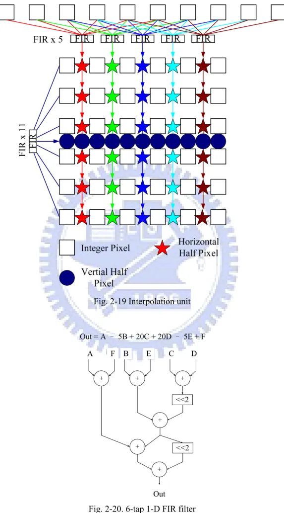
(17) List of Figures Fig. 1-1 The basic structure of encoder. ......................................................... 3 Fig. 1-2 The basic structure of decoder. ......................................................... 3 Fig. 1-3 Organization of this thesis. ............................................................... 9 Fig. 2-1 Block diagram of H.264 motion estimator. .................................... 13 Fig. 2-2 Block sizes and hierarchy for H.264 motion estimation. ............... 13 Fig. 2-3 Integer samples and fractional sample positions for (a) luma and (b) chroma interpolation. ..................................................................... 14 Fig. 2-4 Multiple references in motion estimation....................................... 15 Fig. 2-5 (a) The original coding flow between IME and FME (b) Mode filtering algorithm. ......................................................................... 20 Fig. 2-6 The rate-distortion curves of QCIF sequences. .............................. 22 Fig. 2-7. The rate-distortion curves of CIF sequences. ................................ 22 Fig. 2-8 The rate-distortion curves of 720p sequences. ............................... 24 Fig. 2-9. The three-level new multi-resolution algorithm............................ 26 Fig. 2-10 The rate-distortion curves of 720p sequences. ............................. 27 Fig. 2-11 The rate-distortion curves of 1080p sequences. ........................... 28 Fig. 2-12. The proposed architecture of IME stage. .................................... 31 Fig. 2-13. Basic 4p-SAD unit can accumulate the SAD of four pixels. ...... 31 Fig. 2-14. The SAD calculation unit used for different levels. The modules can process a search point of a 16x16 MB within one cycle. (a) The L0 (Level 0) search point module (b) The L1 (Level 1) search point module (c) The L2 (Level 2) search point module. ............ 32 Fig. 2-15. (a) The 4x4 SAD Tree used in level 0. (b) The 8x8 SAD Tree used in level 1. ............................................................................. 34 Fig. 2-16 The search algorithm of reference software [27] ......................... 39 Fig. 2-17. The proposed SIFME on two square points, (0, 0) and frac_pred_mv, and four triangle point around frac_pred_mv in one quarter-pel distance. .............................................................. 39 Fig. 2-18. The proposed hardware architecture of FME. ............................. 45 Fig. 2-19 Interpolation unit .......................................................................... 46 Fig. 2-20. 6-tap 1-D FIR filter ..................................................................... 46 Fig. 2-21. The block diagram of IME and FME. ......................................... 54 Fig. 3-1 Block diagram of intra-only encoder. ............................................. 59 Fig. 3-2 Nine modes for intra luma 4x4 and 8x8 prediction ........................ 61 xv .

(18) Fig. 3-3 Four modes for intra luma 16x16 and chroma 8x8 prediction ....... 61 Fig. 3-4. Transmission order of all coefficients in a macroblock predicted by 16x16 intra mode. .......................................................................... 61 Fig. 3-5 The scan order and the syntax symbols of a non-zero 4x4 block... 62 Fig. 3-6 Decision flow of (a) original three-step algorithm (b) modified three-step algorithm. ...................................................................... 66 Fig. 3-7 Proposed timing schedule for the modified three-step algorithm. . 67 Fig. 3-8 Proposed architecture of encoder with variable pixel parallelism. 75 Fig. 3-9 Pipelined schedule for fast encoder (a) best luma mode is 16x16 (b) best luma mode is 4x4.................................................................... 78 Fig. 3-10 (a) Eight-pixel parallelism intra prediction generator (b) Examples of operations for intra 16x16 DC mode. ........................................ 80 Fig. 3-11 Eight-pixel parallelism transform unit. ........................................ 80 Fig. 3-12 Inverse transform Unit ................................................................. 82 Fig. 3-13 (a) Quantization and (b) inverse quantization unit ....................... 83 Fig. 3-14 Overall architecture of entropy encoder in H.264 baseline encoder. .............................................................................................................. 84 Fig. 3-15 The overall architecture of CAVLC encoder ................................ 85 Fig. 3-16 An example for nonzero index table: (a) Original 4x4 block and zig-zag scan (b) the initial table after all coefficients are loaded and (c) the updated table after first iteration of leading one detection. ...................................................................................... 85 Fig. 3-17 The cycle reduction by adopted techniques. ................................ 87 Fig. 3-18 The layout and its design specification. ....................................... 88 Fig. 4-1 Profiles of H.264/AVC ................................................................... 95 Fig. 4-2 Nine modes for intra 8x8 prediction. ............................................. 96 Fig. 4-3 Bi-directional motion estimation .................................................... 97 Fig. 4-4 Block diagram of CABAC ............................................................. 98 Fig. 4-5 Flow diagram of arithmetic coding. ............................................. 101 Fig. 4-6 Filtering boundary of a macroblock. ............................................ 101 Fig. 4-7. System overview of H.264 high profile encoder. ........................ 104 Fig. 4-8. The scheduling of H.264 high profile encoder ............................ 104 Fig. 4-9. The schedule of reconstruction module....................................... 106 Fig. 4-10 System architecture of bi-directional motion estimator for H.264 high profile ................................................................................. 107 Fig. 4-11. (a)The architecture of intra encoder part. (b)The gate count reduction of intra encoder by proposed techniques. .................. 109 Fig. 4-12. Intra prediction generator used for intra luma 8x8 modes. ........ 111 xvi .

(19) Fig. 4-13 Pipelined schedule of proposed intra prediction generator ........ 113 Fig. 4-14 Hardware architecture of transform unit .................................... 113 Fig. 4-15 Block diagram architecture of inverse transform unit ................ 115 Fig. 4-16 The architecture of 1-D transform unit ...................................... 116 Fig. 4-17 The 4x4 IDCT transform datapath in inverse transform unit. .... 116 Fig. 4-18 The 8x8 IDCT transform datapath in inverse transform unit ..... 117 Fig. 4-19 The inverse Hadamard transform datapath in inverse transform unit ............................................................................................. 117 Fig. 4-20 Block algorithm of quantization circuits .................................... 118 Fig. 4-21. The architecture of motion estimation part and the proposed algorithms. ................................................................................. 121 Fig. 4-22.(a) The memory access reduction of ME (b) the gate count reduction of ME (c) the internal SRAM buffer reduction of ME (d) The trade-off between the number of search point and quality loss. .................................................................................................... 121 Fig. 4-23 (a) Original serial chedule of CABAC. (b) Modified parallel algorithm for CABAC................................................................ 126 Fig. 4-24 Pipelined CABAC encoding flow .............................................. 126 Fig. 4-25 Architecture of Binarization ....................................................... 127 Fig. 4-26 Architecture of Context Modeling.............................................. 127 Fig. 4-27 Architecture of AC ..................................................................... 127 Fig. 4-28 Architecture of Interval Maintainer ............................................ 128 Fig. 4-29 Architecture of Renormalization ................................................ 128 Fig. 4-30. Architecture design of deblocking filter. ................................... 130 Fig. 4-31. Edge processing order for (A) luma edge, and (B) chroma edge 130 Fig. 4-32. Chip micrograph........................................................................ 133 Fig. 4-33. The power of proposed design and previous works. ................. 135. xvii .

(20) xviii .

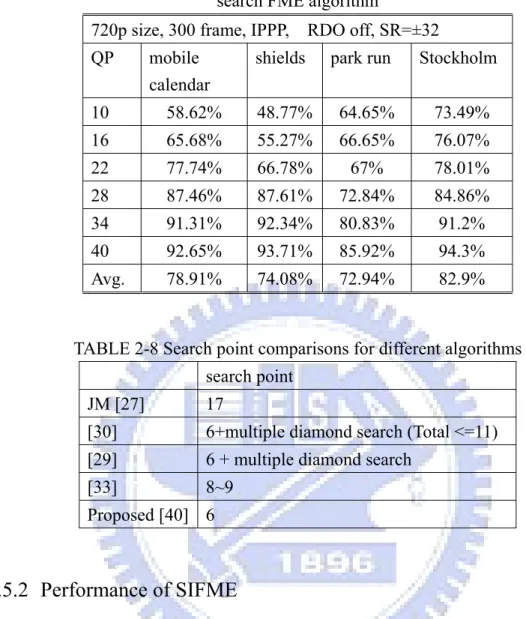
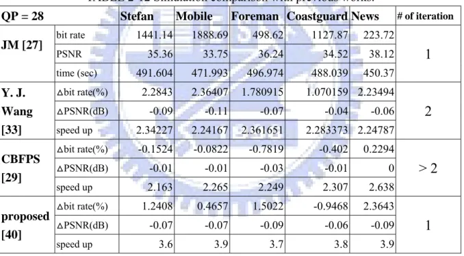
(21) List of Tables TABLE 1-1 Profiles of H.264 Specification .................................................. 6 TABLE 1-2 Levels of H.264 Specification.................................................... 7 TABLE 2-1 The average mode filtering performance for QCIF and CIF sequences ................................................................................. 23 TABLE 2-2. The average mode filtering performance for 720p sequences 24 TABLE 2-3. Performance of PMRME for 720p and 1080p sequences ....... 27 TABLE 2-4. Memory and bandwidth requirement equation for each level. The MBsize is 16. Besides, SRL0, SRL1, and SRL2 are 16, 64, and 256 in respect ........................................................................... 32 TABLE 2-5. Memory and bandwidth requirement is for different frame size. The saving is compared to the direct design [25]. The maximum search range is [-128, 127]...................................... 33 TABLE 2-6 Comparison of the IME part with previous designs. ............... 36 TABLE 2-7 Prediction accuracy of motion vector (mvx and mvy) compared to the full search FME algorithm ............................................. 40 TABLE 2-8 Search point comparisons for different algorithms .................. 40 TABLE 2-9 Simulation results of SIFME for different CIF sequences and QPs when compared to the reference software [27] ................ 42 TABLE 2-10 PSNR and bit rate comparison for different 720p sequences and QPs. Speed up is only the performance in fractional ME part ......................................................................................... 42 TABLE 2-11 PSNR & bit rate comparison for different 1080p sequences and QP .................................................................................... 43 TABLE 2-12 Simulation comparison with previous works. ........................ 43 TABLE 2-13 comparisons of number of processing unit (PU) and number of iterative search steps .......................................................... 45 TABLE 2-14 Comparison of the FME part with previous designs.............. 48 TABLE 2-15 PSNR and bitrate change for proposed algorithms compared with full search for 720p sequences ....................................... 51 TABLE 2-16 PSNR and bitrate change for proposed algorithms compared with full search for 1080p sequences ..................................... 52 TABLE 2-17 hardware cost comparison for complete H.264 ME accelerator with previous works ............................................................... 55 TABLE 3-1 H.264/AVC quantization coefficients ...................................... 70 xix .

(22) TABLE 3-2 H.264/AVC de-quantization coefficients ................................. 70 TABLE 3-3 Probability Distribution of All 16x16 Modes in 720p Sequences with 300 I-frames when QP=28 ............................................... 72 TABLE 3-4 The performance of modified 3-step algorithm and combined algorithm for 720p video sequences. ....................................... 73 TABLE 3-5 The performance of modified 3-step algorithm and combined algorithm for 1080p video sequences. ..................................... 74 TABLE 3-6 Zero-block Codeword Table .................................................... 84 TABLE 3-7 Gate count table for the encoder for HD1080p at 140MHz. .... 87 TABLE 3-8 Comparison with previous intra encoders................................ 90 TABLE 3-9 Comparison of intra predictor part with the state-of-the-art .... 91 TABLE 4-1 Quantization parameter table when QP equals twenty-eight: A for 4x4 block size, B for 8x8 block size ................................ 118 TABLE 4-2 The performance comparison with 4x4 and adaptive Hadamard transform ................................................................................ 123 TABLE 4-3 Optimized codIRange and codILow....................................... 128 TABLE 4-4 Chip specification and features. ............................................. 133 TABLE 4-5 Chip specification and comparison ........................................ 134 . . . xx .

(23) Chapter 1 Introduction The video applications exist in our life in every corner such as the analog/digital broadcast TV, the DVD/Blu-ray video disk, and the streaming video through mobile phone or computer. The video applications provide us a lot of fun and convenience. However, the data amount of the video is very huge. If without compression, no storage device can process these data. Therefore, efficient video compression technique has been proposed to reduce the data size and the bandwidth when transmitting these video signals. The H.264 standard is the latest and the most powerful video compression standard, and many applications adopt this standard. In this chapter, we will review the trends of video coding stand and overview H.264 specification. And then, the motivation of the thesis is proposed and followed by the organization and contribution of the thesis.. 1.1 Overview of H.264 1.1.1 History of H.264 In 1990s, The ISO (International Standard Organization) MPEG4 standard was proposed. for. new. internet-based. video. applications. while. the. ITU-T. (Telecommunication Standardization Sector) H.263 standard for video compression was widely used in videoconference systems. MPEG4 and H.263 are standards based on video compression technology, which are developed by two groups. The one is Motion Picture Experts Group (MPEG) and the other is Video Coding Experts Group (VCEG). In 21th century, both groups were 1 .

(24) in the final stages of developing a new standard that promises to significantly outperform MPEG4 and H.263. The VCEG group started work on two further development areas: a short-term effort to add extra features to H.263 and a long-term effort to develop a new standard for low bit rate video communications. The long-term effort led to the draft “H.26L” standard, offering significantly better video compression efficiency than previous ITU-T standards. Due to the similarity of the groups, in 2001, the Joint Video Team (JVT) was formed by the experts from MPEG and VCEG group. The major task of JVT is to develop the draft H.26L to be a full international standard. Finally, the two identical standards, ISO MPEG4 Part 10 of MPEG4 and ITU-T H.264, were developed. The official title of the new technique is Advanced Video Coding (AVC); however, it is well known by the ITU document number, H.264 [1].. 1.1.2 Introduction of H.264 encoder and decoder Compared to prior video coding standards, many new techniques are employed in H.264 standard and result in significant improvement on coding performance. The details of these techniques can be found in [2]. Here, we would like to give a brief introduction of the basic concepts of the H.264 encoder and decoder. In common with earlier standards, the H.264 standard does not explicitly define a CODEC (encoder / decoder pair). Instead, the standard defines the syntax of an encoded video bit stream together with the method of decoding. Therefore, some variations in encoder is allowed as long as the format of encoded bit-stream is correct. Actually, a compliant H.264 encoder and decoder include the functional modules shown in Fig. 1-1 and Fig. 1-2. In these figures, we can find that the decoder system is. 2 .

(25) Fig. 1-1 The basic structure of encoder. . Fig. 1-2 The basic structure of decoder.. a part of the encoder, whereas there is a certain range for considerable variation in the structure. H.264/AVC also adopts the hybrid video coding scheme which is the same with MPEG 1/2/4. The input video is divided into marcoblocks. A macroblock consists of three components, luma and two chroma components. The luma component presents 3 .

(26) the brightness and the chroma components show the color information. The input macroblocks are predicted by motion estimation (i.e. inter prediction) or intra prediction. If using inter prediction, the macroblock is predicted by the blocks in encoded frames. For intra prediction, the macroblock is predicted by the pixels from neighbor coded macroblocks. The prediction error, which is the difference between the original and predicted pixels, will be transformed and quantized to reduce the value. Finally, the processed predicted error is sent to entropy coding module to generate the final bit-stream. At the same time, the quantized coefficients are reconstructed by inverse quantization and inverse transform and added by the predicted values. The reconstructed image is filtered and stored in the memory as the reference of next macroblock or next frame. Comparing with previous standards, the H.264/AVC standard has these changes: 1. H.264/AVC uses in-loop deblocking filter to replace the post-loop filter in previous standards. 2. H.264/AVC supports multiple references frames. 3. The intra prediction provides higher coding efficiency than previous MPEG-4 standard. 4. The Discrete Cosine Transform (DCT) used in previous standards is replaced by the integer transform. Fig. 1-2 shows the diagram of H.264/AVC decoder. The entropy decoder decodes the quantized coefficients and the motion data. As in the encoder, the prediction pixels are obtained by intra or inter prediction, which is added to the inverse transformed coefficients. The details of the important modules will be introduced in the next chapters.. 4 .

(27) 1.1.3 Profiles and levels of H.264 specification H.264/AVC has many applications; however, different applications have different requirements both in terms of functionalities and complexity. In order to satisfy the requirement of all applications as possible, the H.264/AVC specification defines profiles and levels. A profile is a subset of the coding tools. All decoders compliant to a certain profile must support all the tools of the profile and the syntax format. Now, H.264/AVC standard contains seven profiles, whose supporting tools are listed in TABLE 1-1. However, for many applications, the major difference of requirement between them is the format constrain in resolution and bit-rate, not the supporting tools. Therefore, a level which defines a set of constraints on values of the syntax elements in the bit stream was created for each profile. Each level specifies upper bounds for the bit stream or lower bounds for the decoder capabilities. The difference of all levels is listed in TABLE 1-2. The detailed information on the H.264/AVC profiles and levels can be found in Annex A of [1].. 5 .

(28) TABLE 1-1 Profiles of H.264 Specification Profiles I and P Slices B Slices SI and SP Slices Multiple Reference Deblocking Filter CAVLC CABAC FMO ASO RS Data Partitioning Interlaced Coding 4:2:0 Format 4:0:0 Format 4:2:2 Format 4:4:4 Format 8 Bit Sample Depth 9 and 10 Bit Sample Depth 11 to 14 Bit Sample Depth 8x8 Transform Quantization Scaling Metrices Separate Cb and Cr QP control Separate Color Plane Coding Predictive Lossless Coding. Baseline Yes No No Yes. Extended Yes Yes Yes Yes . Main Yes Yes No Yes . High Yes Yes No Yes . High 10 Yes Yes No Yes . High 4:2:2 Yes Yes No Yes . High 4:4:4 Yes Yes No Yes . Yes. Yes . Yes . Yes . Yes . Yes . Yes . Yes No Yes Yes Yes No No. Yes No Yes Yes Yes Yes Yes. Yes Yes No No No No Yes. Yes Yes No No No No Yes. Yes Yes No No No No Yes. Yes Yes No No No No Yes. Yes Yes No No No No Yes. Yes No No No Yes. Yes No No No Yes. Yes No No No Yes. Yes Yes No No Yes. Yes Yes No No Yes. Yes Yes Yes No Yes. Yes Yes Yes Yes Yes. No. No. No. No. Yes. Yes. Yes. No. No. No. No. No. No. Yes. No No. No No. No No. Yes Yes. Yes Yes. Yes Yes. Yes Yes. No. No. No. Yes. Yes. Yes. Yes. No. No. No. No. No. No. Yes. No. No. No. No. No. No. Yes. 6 .

(29) TABLE 1-2 Levels of H.264 Specification Level Number. Max macroblocks per second. Max frame size (macroblocks). 1. 1485. 99. 1b. 1485. 99. 1.1. 3000. 396. 1.2. 6000. 396. 1.3. 11880. 396. 2 2.1 2.2 3 3.1 3.2 4 4.1 4.2 5 5.1. 11880 19800 20250 40500 108000 216000 245760 245760 522240 589824 983040. 396 792 1620 1620 3600 5120 8192 8192 8704 22080 36864. Max video bit rate (VCL) for all profiles 64-256 kbits/s 128-512 kbits/s 192-768 kbits/s 384-1536 kbits/s 768-3072 kbits/s 2-8Mbits/s 4-16Mbit/s 4-16Mbits/s 10-40Mbits/s 14-56Mbits/s 20-80Mbits/s 20-80Mbits 50-200Mbits 50-200Mbits 135-540Mbits 240-960Mbits. Vertical MV component range [-64,+63.75] [-64,+63.75] [-128,+127.75] [-128,+127.75] [-128,+127.75] [-128,+127.75] [-256,+255.75] [-256,+255.75] [-256,+255.75] [-512,+511.75] [-512,+511.75] [-512,+511.75] [-512,+511.75] [-512,+511.75] [-512,+511.75] [-512,+511.75]. 1.2 Motivation of Thesis H.264 has been adopted as the major coding standard in recently popular high definition video because of its excellent coding efficiency. Due to its high computational loading, ASIC implementation of H.264 encoder is preferred. Therefore, several implementations have been developed [3]-[5], but their performance is limited to baseline 720p [3][4] or SDTV [5]. The main stream 1080p application presents a series of new design challenges in throughput, cost and power because of at least a 4X higher complexity than in the 720p baseline. Thus, in this thesis, we first propose algorithms and architectures for our H.264 encoder to support 1080p resolution without significant quality loss and hardware 7 .

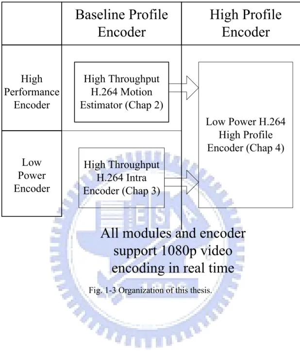
(30) overhead. And then, we integrate the whole design with the new coding tools of high profile to support the latest high definition video applications.. 1.3 Organization and Contribution of Thesis Fig. 1-3 shows the organization and contribution of the dissertation. In chapter 2, we propose a high performance H.264 motion estimator which can support 1080p video with 60fps and the search range up to ±128 without area and throughput overhead [6]. In chapter 3, we provide an alternative solution for application with low power and small area. The high throughput H.264 intra encoder can support 1080p resolution but its area and complexity cost is much lower than original H.264 encoder [7]. Finally, the integrated H.264 high profile encoder combines the high performance and low power techniques from previous two chapters for HDTV applications [8]. The last chapter is the conclusion.. 8 .

(31) High Performance Encoder. High Throughput H.264 Motion Estimator (Chap 2) Low Power H.264 High Profile Encoder (Chap 4). Low Power Encoder. High Throughput H.264 Intra Encoder (Chap 3). Fig. 1-3 Organization of this thesis.. 9 .

(32) 10 .

(33) Chapter 2 High Performance H.264 Motion Estimator for HDTV Motion estimation (ME) part is the most important component in H.264 encoder. In which, the variable block size integer-pel motion estimation (IME) and its improved fractional-pel ME (FME) not only contributes a lot for coding efficiency but also dominates the computational loading of the whole encoding process. Thus, various VLSI realizations of ME have been proposed to speed up the process. In this chapter, we first introduce the motion estimation algorithms of H.264. Besides, we review the previous works and define the problems when extending the supporting resolution to full high definition (HD) size and large search range (SR). And then, we introduce our proposed algorithms and architectures in H.264 motion estimation part for high definition (HD) applications: The first technique, mode filtering (MF), is used to speed up the throughput of whole system. And then the parallel multi-resolution motion estimation (PMRME) reduces the most complexity and memory bandwidth for variable block size motion estimation. Finally, the single iteration fractional motion estimation (SIFME) minimizes the hardware cost and latency for one-quarter fractional motion estimation.. 11 .

(34) 2.1 Introduction to H.264 Motion Estimation 2.1.1 System overview for H.264 motion estimation The H.264 standard adopts the general block-based motion estimation algorithm, which compares the block-based coding data with the reference data to find the best motion vectors. The motion estimation flow of H.264 is illustrated in Fig. 2-1. The current block is compared with the reference data in the search range of previous frames, and the best integer motion vectors are decided by integer motion estimation module. And then the related data is processed by fractional motion estimation modules for refinement. Finally, the residue data which is the difference between current block and best reference block is generated for further coding. Although H.264 standard uses the common block matching algorithm, it has some new features which differ from previous video standards and will be introduced in next sections: z. Variable block size motion estimation. z. Quarter-pel fractional motion estimation. z. Multiple reference frames. 2.1.2 Variable block size motion estimation (VBSME) The H.264 standard adopts hierarchical variable block size (VBS) motion estimation technique to improve the prediction accuracy. Fig. 2-2 shows the block selection procedure and seven possible block size modes for VBSME. In the first step, the best block size is chosen from mode 1 to mode 4 as shown in Fig. 2-2. If the 8x8 mode is preferred, all blocks are split into smaller blocks from mode 4 to mode 7 in the second step. Therefore, there are many combinations of chosen modes in a macroblock. Unlike the previous MPEG 1/2/4 standards which only support 16x16 or 8x8 block matching units, the VBS technique provides flexibility for different 12 .

(35) Fig. 2-1 Block diagram of H.264 motion estimator.. 16 8. ……. 4. ~ Fig. 2-2 Block sizes and hierarchy for H.264 motion estimation.. video sequence. For the video with complex textures, the smaller blocks provide higher coding efficiency. As for the video with flat backgrounds, the larger blocks can predict the video precisely with fewer motion vectors.. 13 .

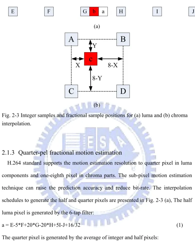
(36) (a). A. B. Y X. c. 8-X. 8-Y. C. D (b). Fig. 2-3 Integer samples and fractional sample positions for (a) luma and (b) chroma interpolation.. 2.1.3 Quarter-pel fractional motion estimation H.264 standard supports the motion estimation resolution to quarter pixel in luma components and one-eighth pixel in chroma parts. The sub-pixel motion estimation technique can raise the prediction accuracy and reduce bit-rate. The interpolation schedules to generate the half and quarter pixels are presented in Fig. 2-3 (a), The half luma pixel is generated by the 6-tap filter: a = E-5*F+20*G-20*H+5I-J+16/32. (1). The quarter pixel is generated by the average of integer and half pixels: b = (E+F+1)/2. (2). As for the chroma part, the sub-pixel in Fig. 2-3 (b) is calculated by the interpolation equation: c= ((8–x)*(8–y)*A+x*(8–y)*B+(8–x)*y*C+x*y*D+32)/32. 14 . (3).

(37) Frame N-4 Frame N-3 Frame N-2. Frame N-1. Frame N. Fig. 2-4 Multiple references in motion estimation.. 2.1.4 Multiple reference frames H.264/AVC standard supports multiple reference frames in motion estimation as shown in Fig. 2-4. At most five frames can be used to predict current block. By this technique, the coding efficiency and prediction accuracy can be further improved. However, the computational complexity is proportional to the number of reference frame.. 2.1.5 Skip mode Because these new techniques in motion estimation stage dominate the computational loading and power of the H.264 encoding process, the most efficient way to lower the complexity and power of H.264 encoder is to skip the prediction procedure of a macroblock and simply use the information of coded macroblock directly. In H.264/AVC, if the following conditions are matched, the macroblock will be skipped and encoded as skip mode: 1.. The chosen block type is 16x16.. 2.. The best motion vector equals the predicted motion vector (MVP).. 3.. The chosen reference frame is the previous frame. 15 . .

(38) 4.. All coefficients are zero after transform and quantization.. 2.2 Design Challenges and Paper Survey 2.2.1 Design challenges As mentioned above, the VBS integer-pel motion estimation (IME) and its improved fractional-pel ME (FME) modules require the most computational resources in the whole encoding process of H.264 standard. Thus many VLSI realizations of ME have been proposed to speed up the process [9]-[18]. However, most of them are only applicable for standard definition (SD) size or below. For high definition (HD) video applications that requires large search range up to [-128, 127] or even larger, direct extension with previous approaches will consume too large area cost, buffers, bandwidth and cycles. To support large search range, many fast integer ME algorithms have been proposed [19]-[24]. However, most of them are not suitable for hardware implementation because of its irregular data flow. Besides, most of these approaches only consider IME or FME only without exploiting their relationship, which may result in extra computation cost. To solve the above problems, we present an efficient ME architecture suitable for HD videos by various design techniques, including a mode filtering algorithm to jointly reduce the IME and FME computations, a parallel multi-resolution ME (PMRME) for large search range IME, and a single iteration FME (SIFME) to achieve the lower cycle count. The cycles are reduced by hardware parallelism and algorithm modification (PMRME and SIFME). Furthermore, we lower requirements of bandwidth and buffer by reusing data within IME as well as between IME and FME. The video quality loss is low by exploiting unequal distribution of motion vectors. With these approaches, we can save more than half of area, bandwidth and 16 .

(39) buffer cost when compared to previous designs.. 2.2.2 Paper survey For fast IME of H.264 standard, various approaches have been proposed [14]-[24] but few can be readily applicable to large search range as used in HDTV. The large search range requirement will result in longer execution cycles as well as large buffer and high memory access. Previous designs with [-63, +64] search range [25][26] use the full search method and thus occupy large area cost. To solve these problems, one promising approach is the multi-resolution ME [14]. In [14], they use three hierarchical levels for search and refine the motion vectors from the coarse level to the finest level. However, the motion vector found in the higher level needs to be further refined in the lower level. It implies the search is a sequential process that will increase the cycle counts, and thus decrease the hardware utilization and throughput. Besides, a full search range sized buffer is still needed because of the dependency between the three hierarchical levels. And then, the required bandwidth is still too large because of poor data reuse of the refinement process. In [15], a modified three-step algorithm is used to decrease the search points for low power, but still consumes large area cost and memory. [16] also uses the subsampling techniques to reduce the hardware cost; however, the two-stage architecture results in longer cycle counts. In [18], the two-stage flow and the irregular search range cause the difficulty of external data transfer. For fast FME, most of them follows the two-step approaches as in reference software [27] which needs total 17 search points for fractional ME. Although this algorithm is suitable for hardware [28], it has two drawbacks. First, the nine search points in each step result in area-costly nine processing units (PUs) for hardware implementation. The second drawback is that it needs two iterative search loops of 17 .

(40) interpolation and Hadamard transform to calculate the SATD cost. To speedup FME, many fast FME [29]-[34] algorithms are proposed to speed up the process. However, these algorithms [29]-[32] are software-oriented, with irregular data flow and thus are not suitable for hardware design. Our previous work [33] is more suitable for hardware and can reduce the processing unit from nine to five to save hardware cost. But all these algorithms suffer from long computation cycles due to the two iterative search loops, one for half-pels and one for quarter-pels. On the other hand, single iteration algorithms like [36][37] have bad performance due to poor interpolation accuracy. The design in [38] increases the throughput by the cost of large area and memory bandwidth. In summary, the hardware implementations of these fast algorithms only reduce the processing element but degrade the quality a lot or do not reduce the total cycle count. These problems will pose strict limits on the HD video applications since FME will take more cycles than IME and thus will dominate the whole pipelining cycle time.. 2.3 Mode Filtering Algorithm 2.3.1 Introduction to mode filtering Fig. 2-5 (a) presents the general flow of IME and FME in the reference software [27] that IME sends the motion vector to FME for refinement. After all possible modes and motion vectors are generated, the best mode and its motion vectors are chosen in the final step of FME. Thus, the IME and FME module both process 41 MVs. To reduce the complexity, we select the two best modes instead of all modes for FME refinement as shown in Fig. 2-5 (b). One mode is chosen from mode 1 to mode 3 in Fig. 2-2, and the other mode is selected from mode 1 to mode 7. With this, only 3 to 18 MVs instead of 41 MVs are computed in FME, which saves 60% to 70% 18 .

(41) computing cycles. In [28], a similar concept but more complex procedure has been proposed. Our method can achieve better quality and lower cycle count than that in [28] because we only select two instead of three candidates and only the best candidate for the 8x8 and smaller subblock case is considered in the final best mode selection. Besides, the method also increases the overall ME pipelining efficiency because it can reduce the cycle count of FME to be similar to that of the IME stage.. 19 .

(42) . (a). (b) Fig. 2-5 (a) The original coding flow between IME and FME (b) Mode filtering algorithm. 20 .

(43) 2.3.2 Simulation result of mode filtering We test the mode filtering algorithm in three different sizes of video: QCIF, CIF and 720p test sequences to see the performances under different conditions. The test sequences with QCIF and CIF resolution are ‘akiyo’, ‘foreman’, and ‘mobile’, which are low motion, medium motion, and high motion sequences respectively. For 720p resolution, the test sequences are ‘Stockholm’, and ‘park_run’. The search ranges are 8, 16 and 32 for QCIF, CIF and 720p sequences respectively. The reference software is JM 9.0 [27] without rate-distortion optimization (RDO). 2.3.2.1 Performance of QCIF/CIF sequences Fig. 2-6 and Fig. 2-7 show the result of mode filtering algorithm for the QCIF and CIF sequences. For small size sequences, we can observe that mode filtering method has similar performance as reference software. TABLE 2-1 presents the average performance of this algorithm of QCIF and CIF sequences respectively. In these results, we find out that the average bit-rate increasing can be only 0.54% and 1.30% and the PSNR degradation is only 0.11db, which performs well. The performances for CIF sequences are better than that for QCIF because the mode filtering technique will filter most of the small block modes while these small block modes are more preferable in small size sequences. Therefore, mode filtering has better performance for CIF sequences because CIF sequences more prefer larger block sizes than QCIF.. 21 .

(44) RD_Curve of QCIF Video 50. 45. PSNR (dB). 40. 35 Foreman_Original Foreman_MF. 30. Mobile_Orig Mobile_MF. 25. Akiyo_Orig Akiyo_MF. 20 0. 500. 1000Bit rate (kbit/sec)1500. 2000. 2500. Fig. 2-6 The rate-distortion curves of QCIF sequences.. RD_Curve of CIF Video 50 . 45 . PSNR (dB). 40 Foreman_Original. 35 . Foreman_MF Mobile_Orig Mobile_MF. 30 . Akiyo_Orig Akiyo_MF 25 0. 1000. 2000. 3000. Bit rate (kbit/sec) 4000 5000. 6000. 7000. Fig. 2-7. The rate-distortion curves of CIF sequences.. 22 . 8000. 9000.

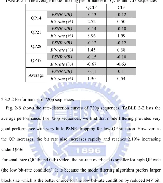
(45) TABLE 2-1 The average mode filtering performance for QCIF and CIF sequences. QP14 QP21 QP28 QP35 Average. QCIF. CIF. PSNR (dB). -0.13. -0.12. Bit-rate (%). 2.52. 0.50. PSNR (dB). -0.14. -0.10. Bit-rate (%). 3.96. 1.59. PSNR (dB). -0.12. -0.12. Bit-rate (%). 1.45. 0.68. PSNR (dB). -0.15. -0.10. Bit-rate (%). -0.67. -0.63. PSNR (dB). -0.11. -0.11. Bit-rate (%). 1.30. 0.54. 2.3.2.2 Performance of 720p sequences Fig. 2-8 shows the rate-distortion curves of 720p sequences. TABLE 2-2 lists the average performance. For 720p sequences, we find that mode filtering provides very good performance with very little PSNR dropping for low QP situation. However, as the QP increases, the bit rate also increases rapidly and reaches 2.19% increasing under QP36. For small size (QCIF and CIF) video, the bit-rate overhead is smaller for high QP case (the low bit-rate condition). It is because the mode filtering algorithm prefers larger block size which is the better choice for the low bit-rate condition by reduced MV bit. For 720p sequences, the frame contents are smoother because of the characteristics of high definition; thus, large block size is preferred in 720p sequences and results in better performance of mode filtering than that in QCIF and CIF video.. 23 .

(46) RD_Curve of 720p Video 50. 45. PSNR (dB). 40. Stockholm_Original. 35. Stockholm_MF 30. Parkrun_Orig Parkrun_MF. 25 1000. Bit rate (kbit/sec) 101000 151000. 51000. 201000. Fig. 2-8 The rate-distortion curves of 720p sequences. TABLE 2-2. The average mode filtering performance for 720p sequences 720p QP12 QP16 QP20 QP24 QP28 QP32 QP36 Average. PSNR (dB). -0.03. Bit-rate (%). -0.45. PSNR (dB). -0.04. Bit-rate (%). -0.71. PSNR (dB). -0.11. Bit-rate (%). -1.37. PSNR (dB). -0.15. Bit-rate (%). -2.30. PSNR (dB). -0.09. Bit-rate (%). -0.42. PSNR (dB). -0.07. Bit-rate (%). 1.23. PSNR (dB). -0.06. Bit-rate (%). 2.19. PSNR (dB). -0.08. Bit-rate (%). -0.26. 24 .

(47) 2.4 Integer Motion Estimation Module : Parallel Multi-Resolution Motion Estimation (PMRME) [35] 2.4.1 Algorithm of PMRME PMRME includes three levels and all of them are independent to each other, as illustrated in Fig. 2-9. In the coarsest level, level 2, the search range (SR) is the largest, [-128~127], and centered on the original point (0,0). This enables the regular memory reuse between successive MB processing as used in most of ME designs [39]. This level uses the 16:1 sampling and thus we only choose the 16x16 mode (mode 1 in Fig. 2-2) since other modes will contain too fewer pixels for SAD calculation and may result in poor mode decision. In level 1, the SR is reduced to [-32 ~ +31] and also centered on (0,0) for memory reuse. This level uses the 4:1 sampling and thus we only choose the 16x16 to 8x8 mode (mode 1 to 4 in Fig. 2-2) for the same reason as level 2. In the finest level, level 0, the SR is set to [-8 ~ +7]. However, unlike the other two levels with (0,0) center, we choose the MVP as the center due to its higher probability to find the final MV here. Thus, we do not subsample data in this level and thus enable search for all variable block size modes. In the three parallel levels, the level 2 provides a large search range for high motion blocks with coarse precision. It is useful for very high motion blocks, and can find a good enough though rough motion vector candidate. Also, the level 1 can provide a. 25 .

(48) Fig. 2-9. The three-level new multi-resolution algorithm.. medium search range but a finer MV precision. With these two large search levels, the motion search algorithm of level 0 can converge to the true motion vector quickly by effects of MVP. If only the level 0 is used, it is difficult to trace the high motion blocks because the MVP cannot follow up the real motion effectively in this case.. 2.4.2 Performance of PMRME TABLE 2-3 shows the video quality of PMRME algorithm for 720p and 1080p sequences respectively. Rate-distortion optimization (RDO) is not used, and only the first frame is intra frame. The search range (SR) is [-128, 127]. All simulation results are compared with reference software JM9.0 [27]. TABLE 2-3 shows the average performance under different QPs. For 720p video, four test sequences are used: Stockholm, park_run, and shields. The frame rate is 30 and 300 frames are coded. 26 .

(49) TABLE 2-3. Performance of PMRME for 720p and 1080p sequences QP. QP16 QP20 QP24 QP28 QP32 Average. 720p. 1080p. PSNR inc.(db). -0.0025. 0.00. Bit rate inc. (%). -1.02. -0.49. PSNR inc.(db). 0. -0.01. Bit rate inc. (%). -0.49. -0.44. PSNR inc.(db). -0.0075. -0.03. Bit rate inc. (%). -0.335. -0.40. PSNR inc.(db). -0.005. -0.06. Bit rate inc. (%). -0.2. 0.40. PSNR inc.(db). -0.01. -0.06. Bit rate inc. (%). 1.56. 1.68. PSNR inc.(db). -0.005. -0.04. Bit rate inc. (%). -0.017. 0.15. RD-Curve for 720p sequences 50. PSNR(dB). 45 Mobcal_Orig. 40. Mobcal_PMRME Parkrun_orig. 35. Parkrun_PMRME Stockholm_orig Stockholm_PMRME. 30. Shield_orig Shield_PMRME. 25 0. 10000. 20000. 30000. 40000. 50000. Bit-Rate(Kbits/sec). Fig. 2-10 The rate-distortion curves of 720p sequences.. 27 . 60000. 70000.

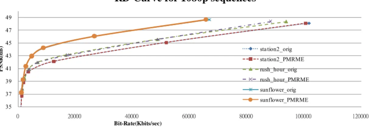
(50) RD-Curve for 1080p sequences 49. PSNR(dB). 47 45. sta tion2_orig. 43. sta tion2_PMRME. 41. rush_hour_orig. 39. rush_hour_PMRME sunflower_orig. 37. sunflower_PMRME. 35 0. 20000. 40000 Bit-Rate(Kbits/sec). 60000. 80000. 100000. 120000. Fig. 2-11 The rate-distortion curves of 1080p sequences.. For 1080p video, three test sequences include: station2, rush_hour, and sunflower. The number of testing frames is 100. We should note that the 1920x1080 image is truncated to 1920x1072 to fit the multiples of 16. Fig. 2-7 and Fig. 2-8 present the rate-distortion curve of 720p and 1080p video sequences, respectively. The results show the PMRME algorithm can achieve the similar video quality as the full search algorithm. However, the bit-rate overhead is larger under high OP because the video quality of reconstructed video will be worse for high QP and the worse reference will mislead the subsampling method. For 720p sequences, PSNR loss is only 0.005dB and the bit-rate decreasing is 1.28% in average. As for 1080p sequences, it has 0.04dB PSNR loss and up to 0.15% of bit-rate decreasing in average. The average PSNR quality loss is negligible and the bit-rate in some cases is decreasing because PMRME also prefers larger block size.. 2.4.3 Architecture of PMRME Fig. 2-12 shows the proposed IME architecture. All three levels can be computed in parallel. A 16x16 current block is shared by three levels. The memory size and bandwidth for three reference frame buffers are listed in TABLE 2-4 and TABLE 2-5. 28 .

(51) The bit width of memory buffer of level 1 and level 2 are truncated while that of the level 0 is not. The reason for this is that the level 0 data can be reused by the following FME hardware if the best MV falls in the level 0. TABLE 2-4 presents the equation of buffer size and the memory access requirement for each level and direct implementation [25]. The MBsize in the table is 16. Besides, SRL0, SRL1, and SRL2 are respective 16, 64, and 256. We should note that the buffer size for direct implementation is the search range size. As for level 0, the buffer size is a little larger than the search range because it includes the neighbor pixels for FME interpolation. But in the case of level 1 and level 2, the memory size is only one-fourth and one-sixteen of their search range by the subsampling techniques. Besides, the bit-truncation technique also reduces 25% to 37.5% buffer size if two or three bits are truncated. As for the memory bandwidth, by the level C data-reuse scheme in [39], the direct implementation needs to update (SR+MBsize-1)*16 pixels. Therefore, the larger search range results in the lower proportion of update rate. Thus, only 16/(64+16) = 20% data in level 1 SRAM should be updated when the coding MB changes with above approach. As for level 2, only 16/(256+16) = 5.88% data should be updated. TABLE 2-5 shows the real buffer size and memory bandwidth requirement for 720p and 1080p video. The proposed algorithm can save over 91.91% buffer in the 720p case and 55% bandwidth in the 1080p case by subsampling and bit-truncation when comparing to [18] that also uses level C data-reuse scheme. If the bus width is 128 bits, it only needs 121 cycles per MB to transfer the required data from external memory to SRAM. In this architecture, all computations are decomposed as the combinations of 4x4 blocks. The basic processing unit is the 4p-SAD (four-pixel SAD) unit which can process the SAD of four pixels as depicted in Fig. 2-13. With this, every level can be easily implemented by regularly composed SAD units. As Fig. 2-12 presents, L0 29 .

(52) (level 0) has one search point module which can process a search point within one cycle so that the level 0 with search range [-8, +7] can finish the full search within 256 cycles. In the same manner, level 1 and level 2 has four and 16 search point modules, which mean the level 1 and level 2 can process four and 16 search points in parallel. Therefore, level 1 and level 2 can process 1024 and 4096 search points within 256 cycles by the parallelization techniques. Fig. 2-14 shows the detailed architecture of search point modules of each level. Fig. 2-14 (a) shows the “L0 search point module”, which is consisted of four row SAD modules. Each row SAD module contains 16 4p-SAD units. Thus, the L0 search point module includes 64 4p-SAD units in total to generate the total SAD cost of a 16x16 MB. As for level 1 with 2:1 subsampling, the number of search point is 1024. Furthermore, since the current buffer for level 1 is also subsampled, only 64 pixels are compared in current MB. Therefore, L1 (Level 1) search point modules in Fig. 2-14(b) only needs 16 4p-SAD units, which is quarter of that in level 0. In order to keep the cycle count of level 1 as the same as that of level 0, we use four L1 search point modules. Thus, four search points in level 1 can be processed in parallel with the same current block. With above arrangement, the total hardware cost of level 1 is the same as that of level 0, 64 4p-SAD units. Similar design considerations are also applied to level 2. Thus, in level 2, the L2 (Level 2) search point module in Fig. 2-14(c) only needs 4 4p-SAD units so that we use 16 L2 search point modules to compute 16 search points in parallel. In summary, all these levels have 64 4p-SAD units respectively to balance the computation cycle of each level to be the same 256 cycles.. 30 .

(53) L2 Search Point Module 0. 67. 19 L2 Search Point Module 1 <<4 L2 Search Point Module 14. 4. L2 Search Point Module 15. 16 39. L1 Search Point Module 0. 8x8 SAD tree 0. L1 Search Point Module 1. 8x8 SAD tree 1. L1 Search Point Module 2. 8x8 SAD tree 2. L1 Search Point Module 3. 8x8 SAD tree 3. L0 Search Point Module 0. 4x4 SAD tree 0. 11 <<2. 8. 31. 16. 16. Fig. 2-12. The proposed architecture of IME stage. C3. C2. C1. C0. R3. R2. R1. R0. Fig. 2-13. Basic 4p-SAD unit can accumulate the SAD of four pixels.. 31 .

(54) L0 Search Point Module. C15 4. C14 4. C13 4. C12 4. C11 4. C10 4. C9 4. C8 4. C7 4 L1 Search Point Module. L2 Search Point Module. C12 4. C8 4. C4 4. C0 4. C12 4. C14 4. C5 4. C10 4. C6 4. C4 4. C8 4. C6 4. C3 4. C2 4. C4 4. C2 4. C1 4. C0 4. C0 4. Fig. 2-14. The SAD calculation unit used for different levels. The modules can process a search point of a 16x16 MB within one cycle. (a) The L0 (Level 0) search point module (b) The L1 (Level 1) search point module (c) The L2 (Level 2) search point module. TABLE 2-4. Memory and bandwidth requirement equation for each level. The MBsize is 16. Besides, SRL0, SRL1, and SRL2 are 16, 64, and 256 in respect Memory cost. buffer size. BW(per MB). Level 0. (SRL0 + MBsize+ 5) * (SRL0+ MBsize + 5)*8. (SRL0 + MBsize +5) * (SRL0+ MBsize+5) *8. Level 1. (SRL1/2 + MBsize/2 -1) * (SRL1/2 + MBsize/2) *(Pixel_DepthL1). (SRL1/2 + MBsize/2 -1) * (SRL1/2 + MBsize/2)* (16/(64+16)) *8. Level 2. (SRL2/4 + MBsize/4 -1) * (SRL2/4 + MBsize/4) *(Pixel_DepthL2). (SRL2/4 + MBsize/4 -1) * (SRL2/4 + MBsize/4) *(16/(256+16)) *8. Direct design. (SR+MBsize-1) (SR+MBsize) *8. (SR+MBsize-1) (SR+MBsize) *(16/(256+16)) *8. 32 .

(55) TABLE 2-5. Memory and bandwidth requirement is for different frame size. The saving is compared to the direct design [25]. The maximum search range is [-128, 127] Memory cost. for 720p. for 1080p. buffer sizeBW(per MB)buffer sizeBW(per MB). Level 0 (Kbyte). 1.369. 1.369. 1.369. 1.369. Level 1 (Kbyte). 0.975. 0.312. 1.170. 0.312. Level 2 (Kbyte) 2.8475. 0.268. 3.417. 0.268. Total (Kbytes). 5.1915. 1.949. 5.956. 1.572. Direct design. 73.712. 4.336. 73.712. 4.336. Saving (%). 92.95. 55. 91.91. 55. The SADs generated from the SAD modules are further summed up by the summation trees to generate the SAD of different block size as shown in Fig. 2-15. In Fig. 2-15(a), level 0 has the most complex summation trees for combination of the seven kinds of block types. The SADs of 4x4 blocks 00, 01, 02, and 03 are accumulated in the first step, and then they are saved to registers dly4. When the SADs of the 4x4 blocks 10, 11, 12, and 13 are ready, these SADs are accumulated for 4x8 and 8x4 SADs. Then two 8x4 SADs are used to generate 8x8 SAD. In the same manner, the SAD of 16x8, 8x16, and 16x16 blocks are generated. For the level 1, four “8x8 SAD tree” are used for combination of the mode 1 to mode 4 block types. Fig. 2-15 (b) presents the 8x8 SAD trees for level 1. However, in level 2, only comparators and registers are needed to select the minimum SAD cost. Finally, the selection module will choose the best two SAD costs from different levels for the fractional ME module.. 33 .

(56) sum4x8 00. sum8x4 00. sum4x4 00. sum4x8 01. sum mode 3. sum8x4 01. sum4x4 01. sum4x8 11. sum8x4 11. sum4x4 11. sum mode 3. sum mode 1. sum mode 2. sum mode 4. 34 . sum mode 1. sum8x4 10. sum mode 2. sum4x8 10. sum4x4 10. . (a). (b) Fig. 2-15. (a) The 4x4 SAD Tree used in level 0. (b) The 8x8 SAD Tree used in level 1..