顧客基礎分析:以一非契約型之線上零售商的顧客購買資訊為例

國立交通大學

管理科學系碩士班

碩士論文

Customer Base Analysis: A Non-contractual Online

Retail Purchase Process Application

顧客基礎分析：以一非契約型之線上零售商的顧客

購買資訊為例

研究生：江品儀

指導教授: 姜齊 教授

唐瓔璋 教授

中華民國九十六年六月

Customer Base Analysis: A Non-contractual Online Retail Purchase

Process Application

顧客基礎分析：以一非契約型之線上零售商的顧客購買資訊為例

研究生：江品儀 Student : Ping-Yi Chiang 指導教授：姜齊 教授 Advisor : Chi Chiang

唐瓔璋 教授 Edwin Tang

國立交通大學 管理科學系碩士班

碩士論文

A Thesis

Submitted to Department of Management Science College of Management

National Chiao Tung University in partial Fulfillment of the Requirements

for the Degree of Master

in

Management Science

June 2007

Hsinchu, Taiwan, Republic of China

Abstract

In this research, we combine the BG/NBD (Fader et al., 2005) and the Extended SMC model (Schmittlein et al., 1994) to simultaneously and completely incorporate the past purchase behavior of customers to do some effective forecasts based on customer base analysis. Differed from the “entire” extended SMC model (based on Pareto/NBD), this research preserves and advocates the easy implementing of the BG/NBD and consider the past dollar volume spent by customers simultaneously by adding the Extended SMC model. Hence, our model is more suitable to be a basis for doing further CLV research than the “pure” BG/NBD, which doesn’t consider any “monetary” information of customers. Furthermore, based on the BG/NBD, we derive the equation of expected active probability for a random chosen customer. It could help us to understand the individual active probability and the true customer base of a firm after summing the active probabilities of all customers. We also empirically validate our model by using a database from an online VCD retailer and try to anticipate the possible purchase patterns of customers in the future both individually and collectively. And we also validate our model results through 1-way MANOVA to test and then we have statistical evidence to approve the differentiation capabilities of the key expected values. Finally, we transform the worksheet of the BG/NBD to a more user-friendly form. With this new worksheet, we only should put the basic purchase history of all customers into and then we could get the expected values of interests at one time. It could save a lot of time to implement this model especially when the base of customers is huge. And the other purpose is that we wish it could improve the utility rate of our model.

Abstract in Chinese

顧客關係管理與一對一行銷不僅是近年來行銷研究領域的熱門議題之 一；實務上，許多企業也紛紛致力於深度經營顧客關係，以減少顧客流失率。 本研究基於顧客關係管理中的顧客基礎分析(Customer Base Analysis)，利用已 知的顧客購買行為(如一定期間內，顧客的購買次數、購買金額、最近一次購買 日)等資訊，透過兩個主要的機率模型的結合：BG/NBD模型(Fader et al., 2005 a) 與Extended SMC模型(Schmittlein et al., 1994)，加上基於BG/NBD模型的假設， 我們推導出原模型並未導出的公式---任一隨機抽取顧客的期望存活率，試圖去 預測未來某段期間內，個別與整體顧客的購買次數、平均單次購買金額及顧客 存活率。同時，我們將使用一家線上日本動畫及影音VCD零售商店的資料庫， 去從事實證分析；並透過單因子多變量分析的驗證，我們發現本模型的三種主 要的預測結果，也可以成為良好的區別龐大顧客群的變數，顯示本研究除了可 以成為未來顧客一生價值分析(Customer Lifetime Value)的基礎模型外，也同時 是企業在落實一對一行銷的良好工具之一。最後，我們將BG/NBD模型原先提 供的工作試算表格式，轉換成為一個更有效率、更方便使用的試算表格式，透 過新的試算表，在輸入已知的顧客過去購買行為後，我們便可在同一時間、一 次得到所有顧客在未來某期間內的預期購買模式。除了可方便模型的使用外， 也期待此舉能更模型廣泛被使用並提高模型的價值。 關鍵字: Pareto/NBD; BG/NBD; RFM; 顧客一生價值

Acknowledgement 兩年的碩士生涯其實過的很快，在這兩年的學習中，很幸運的認識到一群 好同學，尤其是同門的師姐妹，在論文撰寫過程中給予的相互支持與鼓勵。而 最重要的，要十分感謝唐瓔璋老師，在這兩年中總共修習了唐老師所開設的四 門行銷領域的課程，這些課程與大學時期所修習過的行銷課程相比，跳脫千篇 一律的基礎行銷理論介紹，也不再僅以陳腔濫調的公司個案為例，「環球行銷」 提供了一個更具國際觀的視野；「行銷研究專題」介紹了各種行銷相關之統計 分析工具；「行銷工程」也介紹了不同行銷學域的重要理論與基礎模型，而這 篇論文的研究動機，便是來自「行銷工程」中老師所介紹的貝氏統計概念與顧 客關係管理領域中的預測模型。 同時，在論文撰寫的過程中，也感謝老師的細心指導與鼓勵，讓我能夠克 服許多挫折與障礙，並順利找到研究的方向。 最後，我要感謝我的父母以及待在我身邊最重要的人，謝謝他們的支持， 我才能夠奢侈地以非應屆的身份追求這個的碩士學位；當然，我也要將這個碩 士學位，獻給我的父母，謝謝他們賜與我幸福溫馨的家庭生活，讓我無後顧之 憂地放心追逐我的理想；也希望未來我能獻給他們更高的榮耀。

Table of

Contents ABSTRACT ... I ABSTRACT IN CHINESE... II ACKNOWLEDGEMENT...III TABLE OF CONTENTS ... IV LIST OF FIGURES ... VI LIST OF TABLES... VII

1. INTRODUCTION... 1

2. LITERATURE REVIEW ... 3

2.1CUSTOMER RELATIONSHIP MANAGEMENT... 3

2.2DATABASE MARKETING... 4

2.3ONE-TO-ONE MARKETING... 4

2.4CUSTOMER BASE ANALYSIS... 5

2.5CUSTOMER LIFETIME VALUE... 5

2.6THE BENEFITS OF STOCHASTIC CHOICE MODELS... 6

2.7PROBABILITY MIXED MODEL (SCHMITTLEIN,1989) ... 7

2.8THE PARETO/NBDMODEL (SCHMITTLEIN ET AL,1987)... 8

2.8.1 Assumptions... 8

2.8.2 Model Specification... 9

2.8.3 Key Mathematical Results... 10

2.8.4 Related Key Points about the Pareto/NBD Model ... 12

2.9THE BG/NBDMODEL (FADER ET AL,2005 A)... 12

2.9.1 Assumptions... 12

2.9.2 Key Mathematical Results... 14

2.9.3 Related Key Points about the BG/NBD Model ... 15

2.10THE EXTENDED SMCMODEL (SCHMITTLEIN ET AL,1994)... 16

2.10.1 Assumptions... 16

2.10.2 Key Mathematical Results... 17

2.10.3 Related Key Points about the Extended SMC Model ... 18

3. CONCEPTUAL FRAMEWORK ... 19

3.1ASSUMPTIONS... 19

3.1.1 Terms Definition... 19

3.1.2 Assumptions... 20

3.2MODEL DEVELOPMENT FOR A RANDOMLY CHOSEN CUSTOMER... 22

3.2.1 Expected Number of Transactions ... 22

3.2.2 Expected Active Probability ... 22

3.2.3 Expected Dollar Volume per Reorder ... 24

4. EMPIRICAL ANALYSIS ... 25

4.1DATA DESCRIPTION... 25

4.2.1 Transaction/Dropout Process... 26

4.2.2 Transaction Dollar Volume ... 28

4.3MODEL RESULTS... 29

4.3.1 Expected Number of Reorders (Conditional Expectation)... 29

4.3.2 Expected Active Probability ... 33

4.3.3 Expected Dollar Volume per Reorder ... 35

4.4INTEGRATED INDIVIDUAL CUSTOMER FORECASTS... 36

4.5COLLECTIVE CUSTOMER FORECASTS... 37

4.6MODEL VALIDATION... 37

4.6.1 1-Way MANOVA... 38

4.6.2 Validation Result ... 41

5. CONCLUSION AND DISCUSSION... 42

5.1RESEARCH CONTRIBUTION... 42

5.2RESEARCH LIMITATION... 42

5.3FUTURE RESEARCH DIRECTION... 43

List of Figures

Figure1. Screenshot of Excel Worksheet of Raw Data……….26 Figure2. Screenshot of Excel Worksheet of Parameter Estimation………...27 Figure3. Screenshot of Excel Worksheet of Conditional Expectation………..31 Figure4. Screenshot of Excel Worksheet of Conditional Expectation—New Version…….32 Figure5. Screenshot of Excel Worksheet of Expected Active Probability………34 Figure6. Screenshot of Excel Worksheet of Expected Dollar Volume………..35 Figure7. 1-Year Predictions for Illustrative Customer Accounts………..36

List of Tables

Table1. Correlation between Forecast Period Transaction Numbers………16

Table2. Model Estimation Results of Transaction/Dropout Process……….27

Table3. Model Estimation Results of Transaction Dollar Volume….………..….29

Table4. 1-way MANOVA Test Result---Overall Test………...38

Table5. 1-way MANOVA Test Result---Marginal Test---EY………39

Table6. 1-way MANOVA Test Result---Marginal Test---EZ………....40

Table7. 1-way MANOVA Test Result---Marginal Test---PRO……….40

1. Introduction

Customer relationship management (CRM) is becoming a central research paradigm in the marketing channel literatures (Heide, 1994). Within the so many research regions, database marketing is one facet of CRM. And it’s also one instrument to implement CRM. If a company can address and target individual customers to implement one-to-one marketing, it can improve its profitability by serving these customers differently (Niraj et al. 2001). Customer base analysis is one part of database marketing and is also one tool to implement one-to-one marketing. In this research, we utilize some stochastic choice models to analyze a customer base of an online retailer and hope to predict future purchase behavior of the customers. Besides, if we want to calculate the lifetime value (LTV) of a customer, customer profitability models of current period costs and revenues as well as forecasting models of future revenues and costs are required (Niraj et al., 2001). Because our model is belonged to a forecasting model, it would be help to calculate the LTV of customers.

In this research, based on customer base analysis, we will implement two stochastic choice models by using a non-contractual online retail database. In a non-contractual setting, the time at which a customer becomes inactive is unobserved. The big challenge that faces non-contractual marketers is how to differentiate some customers who have indeed ended their relationship with a firm from other customers who are just in the midst of a long hiatus between transactions. In conclusion, we will use a transaction database from an online retail to empirically validate several stochastic choice models and intend to solve the following questions:

♦ Which individuals in this database are most likely to be active or inactive in the future?

♦ What level of transactions measured individually or collectively should be expected in the future?

expected in the future?

Although the first question was the key issue of the Pareto/NBD model (Schmittlein et al., 1987), it could not be solved by the BG/NBD model (Fader et al, 2005 a) because the authors of this model did not derive the active probability function for a randomly chosen customer. So we will try to derive it based on the BG/NBD model and answer the first question. The last one could not be solved either by the BG/NBD model alone. Thus we will incorporate dollar volume by using the normal-normal mixture model jointly (also called the extended SMC model) (Schmittlein and Peterson, 1994) to increase the practical utility of the original BG/NBD model.

This paper is organized as follows. Section 2 presents an overview of literature about many constructs which have been mentioned above and three probability models for customer base analysis. Section 3 specifies our conceptual framework. In our framework, the main stochastic model is based on the BG/NBD model to

capture the flow of transactions over time and a normal-normal mixture for spend per transaction. We will integrate the two models and try to develop an equation to capture the customer active probability based on BG/NBD model. Of course, we expected it could also be utilized in Microsoft Excel as well and it’s also one of the contributions of the BG/NBD model especially for marketing practitioners. Section 4 empirically implements the models with a non-contractual online retail database and utilizes 1-way MANOVA to validate our model results. In section 5, we

conclude with several issues that arise from this work, review several limitations in our research and suggest some future research directions.

2. Literature Review

2.1 Customer Relationship Management

The definitions of CRM in many literatures are a little bit different. One definition of CRM is utilizing software and other related technologies to automate and improve business processes in areas of sales, marketing, customer service and etc. Another one is that CRM is a measure for an organization to acquire new customers, retain original customers and increase the profitability of customers through continuous communications to understand and influence the behavior of customers. To sum it up in a sentence, we can say that CRM is an approach which uses data mining, information technology and integrated marketing communication to understand and communicate with customers and then influence their behavior. The ultimate objectives are increasing market share, decreasing churn rate of customers, recapturing lost customers and enhancing customer lifetime value.

CRM research can be organized along the customer lifecycle, including customer

acquisition, development and retention strategies (Kamakura et al., 2005). Customer acquisition extends from the channels customers use to first access the firm (Ansari

et al., 2004) to the promotion that bring them to the firm. If a firm uses appropriate

development strategies such as delivering customized products (Ansari and Mela,

2003) and cross-selling (Kamakura et al., 1991 and 2003), it can enhance the value of a customer from the firm. Early detection and prevention of customer churn can also enhance the total lifetime of the customer, if a firm can put efforts on the

retention of valuable customers (Kamakura et al., 2005).

Why has CRM caught so much attention? One reason is that customer relationship management is a natural evolution from well-established market segmentation and target-marketing activities (Essential readings in marketing, MBR). Last but not least, if a firm implements CRM, profits will have some increase.

Profits can increase because of several reasons (Reichheld, 1996). First, by applying retention programs, customers are confronted with increasing switching

costs so they have fewer incentives to change their current behavior (Jones et al., 2000). Secondly, the longer a customer stays, the more he spends at the company. Otherwise they may be likely to convince others about the positive value the company offers (word-of-mouth effect). And they tend to be less price sensitive (Zeithaml et al., 1996) and would be less responsive to competitive pull (Stum and Thiry, 1991). All these could greatly promote the firm’s profitability.

2.2 Database marketing

Database marketing is using information technology to construct and maintain a database system consisting of related information of current and latent customers. Then a company could exploit this database to provide customers better products or services. The most important one is to build long term relationships with them. In this way, a company could build up customer loyalty, decrease wasting of resources and enhance the customer satisfaction toward the company (Hughes, 1994).

2.3 One-to-one marketing

One-to-one marketing means being willing and able to change on what the customer tells you and what else you know about that customer (Peppers et al., 1999). Practiced correctly, one-to-one marketing can increase the value of the customer base of firms (Niraj et al. 2001). One-to-one marketing focuses on customer satisfaction and is customer-oriented (Weng and Liu, 2004). To implement one-to-one marketing, it is necessary to (a) identify customers; (b) differentiate customers; (C) interact with customers; and (d) personalize products or services to tailor-suit customers (Peppers et al., 1999).

2.4 Customer base analysis

Customer base analysis is concerned with using the observed past purchase behavior of customers to understand their current and likely future purchase patterns (Schmittlein and Peterson, 1994). Importantly, many choice modelers often find purchase history to be much more predictive than marketing mix variables such us price or promotions (Fader and Lattin, 1993; Guadagni and Little, 1983). In so many aspects that CRM puts emphasis on; customer base analysis especially focuses on retained customers. Retained customers could produce higher revenues and margin than new customers (Reichheld and Sasser, 1990). And a 1% improvement in retention can increase firm value by 5% (Gupta et al., 2004). Therefore it’s reasonable and supported that firms should spend more marketing resources to retain existing customers rather than acquiring new ones (Rust and Zahorik, 1993; Mozer et al., 2000).

2.5 Customer Lifetime Value

In this customer-centric era, firms should focus on building and managing customer equity and not just brand equity. Customer equity is the sum of lifetime values (LTVs) of customers, where each customer’s LTV is the sum of the properly discounted stream of net profits from the customer over the lifetime of the customer-firm relationship (Blattberg and Deighton, 1996). Customers generally interact with a firm over multiple periods. If we want to calculate the LTV of a customer, customer profitability models and forecasting models are required (Niraj et al., 2001). Within the two aspects, it’s more complex to estimate future revenues and costs. Forecasting models, also called stochastic choice models, have been advanced to predict the likelihood of future events based on past history in marketing literature. Because they can be used to identify the likelihood of current customers being active in the future and to predict future revenues, they play an

important role in the calculation of LTV of customers.

2.6 The benefits of stochastic choice models

First of all, the development and application of stochastic choice models could help to formulate and adopt customer retention strategies, which belong to one scope of CRM research. Secondly, through utilizing stochastic choice models, it’s one of the methods to identify and differentiate customers, which are the first two steps to implement one-to-one marketing. Thirdly, because of the forecasting capability of the stochastic choice models, they also take a big responsibility for the expectation and calculation of LTV of customers.

Although in our framework the main stochastic model is based on the BG/NBD model, the creative motivation behind the BG/NBD model was looking forward to be approximated to the Pareto/NBD model. Thus, the behavioral stories of the two models are almost close to each other.

The Pareto/NBD model (Schmittlein et al., 1987) is a benchmark model for customer-base analysis in a non-contractual setting. But its empirical application can be challenging, especially in terms of parameter estimation (Fader and Hardie, 2005 a). It’s also one of the reasons for us to choose the BG/NBD model as the main stochastic model.

In this following, before the complete introduction of the models, we will show the basic form of a probability mixed model. Because all the three following models are categorized to probability mixed models. And then we will respectively introduce the Pareto/NBD model, the BG/NBD model and the normal-normal mixture (also called the extended SMC model) (Schmittlein and Peterson, 1994) in order.

2.7 Probability Mixed Model (Schmittlein, 1989)

Some models have been called probability mixture models, since they envision a mixture across individuals of heterogeneous probabilistic processes. Such a mixture model consists of two components. First, events for individuals are assumed to follow some stochastic process whose form is specified up to some parameter θ (which may be a vector), and second, the stochastic process observed may vary across individuals. And usually the general form of the process is assumed to remain the same over individuals, so the variation can be thought of as a distribution for the latent trait θ over the population. Then, letting a random variable X associated with an individual have a cumulative distribution functionF(X θ)and the variation in θ over the population have a distribution functionG(θ γ).

The distribution of X for an individual chosen at random is

∫

−∞∞

=

(

)

(

)

)

(

X

γ

F

X

θ

dG

θ

γ

H

And the population mean is

∫ ∫

−∞∞ ∞ ∞ −

=

x

dF

(

x

θ

)

dG

(

θ

γ

)

u

Thus, for an individual, the expectation of X conditioned on the latent trait θ is

[ ]

_∫

∞ ∞ −

=

≡

(

)

)

(

θ

E

X

θ

x

dF

x

θ

J

Therefore, given an initial observation that X=x, the conditional expectation of this

characteristic (denoted by_X*_{) is}

[

]

[

]

∫

−∞∞

=

=

=

=

=

)

,

(

)

(

)

(

*

x

X

dG

J

x

X

J

E

x

X

X

E

γ

θ

θ

θ

θ

whereG(θ γ,X =x)is an updated distribution of θ given the observation X=x. Within a Bayesian framework,G(θ γ)is the prior distribution while G(θ γ,X =x)is the posterior. Consequently, the researchers may observe X-values of many

heterogeneous individuals and use these values to estimate the distribution )

(θ γ

G (Morris, 1983).

After understanding the prototype of a probability mixed model, we hope it could help to comprehend the model developments of the three following models. Hereafter, we will specify the assumptions and development of the three models separately.

2.8 The Pareto/NBD Model (Schmittlein et al, 1987)

Before we introduce the Pareto/NBD model, we’ll make some definitions for the concepts we’ll mention later. This model will consider only purchasing or transaction events. That is, the amounts purchased by customers won’t be considered in the model development. Each transaction event will be termed a “purchase.” A customer who is still active will be termed “Alive,” while a customer who has left for whatever reason will be termed “Dead.” The observation time of a customer who is still alive at time 0 is T. During T of a customer, the customer will have made X purchases with the last purchase coming at t, 0＜t≦T. Hence, the information on this customer contains 3 elements:

Information = (X, t, T).

After these concepts have been defined, we will introduce the basic assumptions and the development processes of the Pareto/NBD model.

2.8.1 Assumptions

(1) Transactions by active customers

While active, the number of transactions X, made by each customer in time period of length t is a Poisson random variable with a purchase rate λ:

[

]

( )

[

]

[

]

, ; 0,1, 2.... ! , , , x T T P X x T e x x E X T T Var X T T λ

λ

λ τ

λ τ

λ

λ τ

λ

− = > = = > = > =

(2) Individual customer retention/dropout

Each customer has an unobserved “lifetime” of length τ which is an exponential random variable with a dropout rate µ:

(

)

[ ]

[ ]

2 ; 0 1 1 f e E Var µτ

τ µ

µ

τ

τ µ

τ µ

µ

µ

− = > = =

(3) Heterogeneity in purchase rates

The purchase rate λ of different customers follows a gamma distribution across the population of customers with shape parameter γ and scale parameter α:

(4) Heterogeneity in dropout rates

The dropout rate µ of different customers follows a gamma distribution across the population of customers with shape parameter s and scale parameter β:

(5) Rates λ and µ are independent

The purchase rate λ and dropout rat µ vary independently across customers.

2.8.2 Model Specification

(1) Purchase event model---NBD model

Based on assumption (1) & (3), purchases made by a sample of customers while they are active follow the NBD model (Poisson mixed with Gamma)

(

_,

)

_{( )}

1

_;

_0;

_,

₀

g

e

γ γ αλ

α

λ γ α

λ

λ

γ α

γ

− −

=

>

>

Γ

(

_,

)

_{( )}

s s 1

_;

_0;

_,

₀

h

s

e

s

s

βµ

β

µ

β

₌

µ

− −

µ

_>

β

_>

Γ

(Ehrenberg, 1972).

[

_{, ,}

]

1 _{; 0,1, 2....} r x x x T P X x T C x T T γ

α

γ α τ

α

α

+ − ⎛ ⎞ ⎛ ⎞ = > = _{⎜ ⎟ ⎜ ⎟} = + + ⎝ ⎠ ⎝ ⎠

(2) Duration model---Pareto model

Based on assumption (2) & (4), the lifetime “τ” of a sample of customers follows the Pareto distribution of the second kind (Exponential mixed with Gamma) (Johnson and Kotz, 1970).

(

)

₍

₎

(

)

1 , , 0; , , 1 1 s s f s E s s s β τ β _{β τ} τ β β τ β + ⎛ ⎞ = _{⎜ + ⎟} > ⎝ ⎠ = > −

(3)Thus, this combined purchase event model and duration model will be called the Pareto/NBD model. It has four parameters: γ, α, s and β

2.8.3 Key Mathematical Results

There are the key results that derived from the above-cited distributions below.

(1) The expected number of purchases in a time period of length T for a randomly chosen customer is

(2) The probability for a randomly chosen customer being active in a time period of length T is

The result varies depending on the values of α and β. There are three conditions.

[

, , , ,

]

₍

₎

1 1 1 s E X s T s T γβ β γ α β α β − ⎡ _{⎛ ⎞} ⎤ = ⎢ −_{⎜ ⎟} ⎥ − _{⎢⎣ ⎝} + _{⎠ ⎥⎦}

[

]

[

]

(

)

0 0 , , , , , , , , , , , , , , , , , P T s X x t T P T X x t T f r s X x t T d d τ γ α β τ λ µ λ µ α β λ µ ∞ ∞ > = =

∫ ∫

> = =

Case 1: α＞β

[

]

( )

(

)

(

( )

)

1 1 1 1 1 1 1 1 1 , , , , , 1 , ; ; , ; ; x s s P T s X x t T s T T T F a b c z t F a b c z t x s t t T γ τ γ α β α β β γ α α α − + > > = ⎧ ⎡ _{+ + +} ⎤⎫ ⎪ ⎛ ⎞ ⎛ ⎞ ⎛ ⎞ ⎪ =⎨ + _{+ +} ⎢_⎝⎜ ₊ ⎟_⎠ ⎜_{⎝ +} ⎟_⎠ −_⎝⎜ ₊ ⎟_⎠ ⎥⎬ ⎢ ⎥ ⎪ ⎣ ⎦⎪ ⎩ ⎭

( )

1 1 1 1 ; 1; 1; where a x s b s c x s z y y γ α β γ α = + + = + − = + + + = + Case 2: α＜β

[

]

( )

(

)

(

( )

)

1 2 2 2 2 2 2 2 2 , , , , , 1 , ; ; , ; ; x s r x P T s X x t T s T T T F a b c z t F a b c z t x s t t T γ τ γ α β α β α γ β β β − + + > < = ⎧ ⎡_{⎛ + ⎞ ⎛ + ⎞ ⎛ + ⎞} ⎤⎫ ⎪ ⎪ =⎨ + _{+ +} ⎢⎜ ₊ ⎟ ⎜ ₊ ⎟ −⎜ ₊ ⎟ ⎥⎬ ⎝ ⎠ ⎝ ⎠ ⎝ ⎠ ⎢ ⎥ ⎪ _{⎣ ⎦}⎪ ⎩ ⎭

( )

2 2 2 2 ; ; 1; where a x s b x c x s z y y γ γ β α γ β = + + = + − = + + + = + Case 3: α＝β

[

]

1 , , , , , 1 1 x s P T s X x t T s T x s t γ τ γ α β α γ α − + + > = = ⎧ ⎡ ₊ ⎤⎫ ⎪ ⎛ ⎞ ⎪ = +⎨ _{+ +} ⎢⎜_{⎝ +} ⎟_⎠ − ⎥⎬ ⎢ ⎥ ⎪ ⎣ ⎦⎪ ⎩ ⎭

In case 2&3, is the Gauss hyper-geometric function

(Abramowitz and Stegun, 1972, p.558). It can be computed using either numerical integration or the algorithms. The authors of the Pareto/NBD model used numerical integration to compute the Gauss hyper-geometric function.

(3) The expected number of purchases in a future period of length T* for a randomly chosen customer is

* _{, , , , , , ,} * * _{, , , ,} * _{, , , , , ,}

E X_⎣⎡ γ α βs X=x t T T ⎤_⎦=E X_⎣⎡ γ +xα+T s β+T T _⎦⎤× ⎡ >P_⎣τ T γ α βs X =x t T⎤_⎦

(

a b c z

)

2.8.4 Related Key Points about the Pareto/NBD Model

♦ The likelihood function associated with the Pareto/NBD model is very complex because it involves many evaluations of the Gaussian hyper-geometric function. These multiple evaluations of the Gaussian hyper-geometric function are not only unfamiliar to most researchers working in the areas of database marketing and CRM analysis but are quite demanding from a computational standpoint (Fader et al., 2005).

♦ In the only published paper which successfully implemented the Pareto/NBD model by Reinartz and Kumar in 2003, the estimations of parameters have ever been commented on the associated computational burden as well(Reinartz and Kumar, 2003).

2.9 The BG/NBD Model (Fader et al, 2005 a)

2.9.1 Assumptions

The only difference between the Pareto/NBD model and the BG/NBD model lies in the behavior story about how or when customers become inactive. The Pareto/NBD model assumes that dropout can occur at any point in time whether or not actual purchases are taking place. However the BG/NBD model should be based on an assumption that dropout could only occur after an occurrence of an actual purchase and then we could model this process using the beta-geometric (BG) model.

The concepts such as “purchase”, “Alive”, “Dead” and “T” are defined the same as them in the Pareto/NBD model. The observation time of a customer who is still alive at time 0 is T.

There are also five assumptions behind the BG/NBD model.

(1) Transactions by active customers

period of length t is a Poisson random variable with a purchase rate λ. It equals to assume that the time between transactions is distributed exponential with the same purchase rate λ:

(2) Individual customer retention/dropout

After any transaction, a customer could become inactive with a dropout rate p. So the point at which a customer becomes inactive follows a geometric distribution with dropout rate p:

(3) Heterogeneity in purchase rates

The purchase rate λ of different customers follows a gamma distribution across the population of customers with shape parameter γ and scale parameter α:

(4) Heterogeneity in dropout rates

The dropout rate p of different customers follows a beta distribution across the population of customers with two parameters a and b:

(5) Rates λ and p are independent

The purchase rate λ and dropout rate p vary independently across customers.

Thus, based on assumption (1) and (3), the transaction model also belongs to the NBD model. And based on assumption (2) & (4), the retention model belongs to the BG model. This small and relatively inconsequential change to the original Pareto/NBD assumptions does not require any different psychological theories, nor does it have any

(

)

( ) 0 , ; ₁ 1 1 > ≥ = − − ₋ − − j j t t j j t e t t t f

λ

λ

λ j j

(

)

(

1−

)

1, =1,2,3,... = − j p p n transactio jth after y immediatel inactive P j

(

,

)

_{( )}

, 0 1 > Γ = − − λ γ λ α α γ λ γ γ e λα f

(

)

(

₍

₎

)

, 0 1 , 1 , 1 1 ≤ ≤ − = − − p b a B p p b a p f b a

noteworthy managerial implications (Fader et al., 2005 a).

2.9.2 Key Mathematical Results

(1) The expected number of purchases in a time period of length t for a randomly chosen customer is

(2) The probability for a customer being still active at a point of time t is

(3) The expected number of purchases in a future period of length t for a randomly chosen customer is

(4) The likelihood function for a randomly chosen customer with purchase history (X, tx, T)

( )

(

)

⎥ ⎥ ⎦ ⎤ ⎢ ⎢ ⎣ ⎡ ⎟ ⎠ ⎞ ⎜ ⎝ ⎛ + − + ⎟ ⎠ ⎞ ⎜ ⎝ ⎛ + − − − + = t t b a b F t a b a b a t X E α γ α α α γ γ ; 1 ; , 1 1 1 , , , 2 ₁

( )

(

)

x x x x x t T x b a t T t x b a x b x F t T T a x b a b a T t x X t Y E + > + ⎟⎟ ⎠ ⎞ ⎜⎜ ⎝ ⎛ + + − + + ⎥ ⎥ ⎦ ⎤ ⎢ ⎢ ⎣ ⎡ ⎟ ⎠ ⎞ ⎜ ⎝ ⎛ + + − + + + + ⎟ ⎠ ⎞ ⎜ ⎝ ⎛ + + + − − − + + = = γ γ α α δ α γ α α α γ 1 1 ; 1 ; , 1 1 1 , , , , , , 0 1 2

(

)

(

)

(

) ( )

t p j t j j

e

j

e

t

p

p

t

at

active

P

t

P

λ λ

λ

λ

τ

− ∞ = −

=

−

=

=

>

∑

0

!

1

,

(

)

(

)

( )

( )(

(

)

)

(

( )

)

( )(

(

)

)

(

)

(

)

( )

( ) (

(

) (

)

)

x x x x x x x x x t x b a A T A x b a b x b b a A x A where A A A A t x b a B x b a B T x b a B x b a B T t x X b a L + + > + > + ⎟⎟ ⎠ ⎞ ⎜⎜ ⎝ ⎛ + ⎟ ⎠ ⎞ ⎜ ⎝ ⎛ + + = ⎟ ⎠ ⎞ ⎜ ⎝ ⎛ + = + + Γ Γ + Γ + Γ = Γ + Γ = + ⋅ ⋅ = + Γ + Γ − + + + + Γ + Γ + = = γ γ γ γ γ γ γ α α γ α γ δ α γ α γ δ α γ α γ α γ 1 1 , 1 , , , 1 , 1 , , , , , , , 4 3 ' 2 1 4 0 3 2 1 0

In order to implement the likelihood function in Microsoft Excel, the authors rewrote the original one and used A1~A4 to replace it.

(5) The sample log-likelihood function

Then suppose we have a sample of N customers, where customer i has transactions Xi=xi in the time period (0, Ti] and their last transaction occurs at txi.

Thus the sample log-likelihood function is

(

)

_∑

[

(

)

]

=

=

=

N i i x i i

x

t

T

X

b

a

L

b

a

LL

_i 1

,

,

,

,

,

ln

,

,

,

α

γ

α

γ

By this function, the authors of the BG/NBD model use the method of maximum likelihood to estimate the four parameters γ, α, a and b.

2.9.3 Related Key Points about the BG/NBD Model

♦ It’s easy to implement the BG/NBD model because we could operate the whole model with a standard spreadsheet package (Excel), even the estimation of parameters.

♦ In the BG/NBD model, the authors didn’t derive the formula about the probability that a random chosen customer is still active at a point of time t ( ). It will somewhat diminish its usefulness if we want to know the size of the currently active customer pool and the rate at which that pool’s size is increasing or decreasing. Therefore, to derive the formula is one of our main contributions in this research paper. ♦ One of the reasons that the authors wanted to develop the BG/NBD model

(

t

)

P

(

activeatt a b

)

Pτ > = γ,α, ,

was to approximate the Pareto/NBD model. From the table 1 we could make a conclusion that the approximation effect is impressively good. (The

table comes from (Fader et al.,2005 a))

Table 1 Correlation Between Forecast Period Transaction Numbers

2.10 The Extended SMC Model (Schmittlein et al, 1994)

The Extended SMC model is a normal-normal mixture model and it incorporates

dollar volume of transactions made by customers. This model got this name just because one of the builders of the Extended SMC model was the same with the one of the Pareto/NBD model, also called SMC model, and this model could also compensate the drawback of the Pareto/NBD model that didn’t consider the dollar volume of transactions. This model has three assumptions shown below.

2.10.1 Assumptions

For a customer observed to have X reorders in a time period, they let Zi denote

the dollar volume of per order i (i=1,…, X)

(1) Individual customer level

The set of Zi are i.i.d. normal random variables with mean θ and varianceσ W2 which represents the variance in the dollar volume spent across reorders for a customer and is constant across customers.

(2) Heterogeneity

Mean θ is assumed to vary across customers according to a normal

distribution with mean and variance which represents the variance in average dollar volume spent across customers.

θ

～

N( , )

(3) Rates λ, µ, and θ are independent from each other

The average amount spent θ, the purchase rate λ and the dropout rate µ vary independently across customers where λ and µ have been clearly defined in the Pareto/NBD model.

Thus, based on assumption (1) and (2), the Extended SMC model belongs to a normal-normal mixture model.

2.10.2 Key Mathematical Results

(1) The reliability coefficient that the confidence one could place in a single observed dollar volume Zi of past order is (relative to rely on the population average dollar volume ):

(2) If the observed number of reorder equaled to 1, X=1, the best estimate for θ is (Schmittlein, 1989):

(3) If X≧1, the reliability coefficient of is:

(4) The expected future volume per reorder is:

[ ]

θ

E

σ

A2

[ ]

θ E

σ

A2 2 2 2 1 W A A

σ

σ

σ

ρ

+

=

[ ]

θ E

[ ]

θ

Z

ρ

Z

(

ρ

)

E

[ ]

θ

E

₁

=

_{1 1}

+

1−

₁

∑

= = X i i Z X Z 1 1

(

_W X

)

A A X 2 2 2

σ

σ

σ

ρ

+ =

[

θ

Z Z

]

X

σ

Z

σ

E

[ ]

θ

E ₌⎛ A ⎞ ₊⎛ A ⎞ 2 2 ,...,

(5) For a customer with a given purchase information (X, t, T, Z), the expected future dollar volume could be multiply “the expected future volume per reorder” (Schmittlein et al, 1994) by “the expected number of purchases in a future period of length T*” (Schmittlein et al, 1987).

2.10.3 Related Key Points about the Extended SMC Model

♦ The first two assumptions in the Extended SMC model were convenient but unnecessary. Because the formula, “the expected future volume per reorder”, could also be derived from the standpoint of minimizing squared prediction error in θ without the normality assumptions (Gerber, 1979, Chapter 6).

♦ Thus the third assumption is a “true” constraint when we use the model. In the original paper (Schmittlein et al, 1994).

♦ Although the Extended SMC model was named like this, the estimation of the parameter θ and the model development had no relationship with the four parameters in the Pareto/NBD model (SMC model). The three basic assumptions of the Extended SMC model could also be hold the same while we use the BG/NBD model to substitute for the Pareto/NBD model in the recommended computation formula of “the expected future dollar volume”.

Thus in our following framework, we will use the BG/NBD model to capture the transaction/dropout process of customers and the Extended SMC model to incorporate the dollar volume of transactions.

3. Conceptual Framework

This research will be based on customer base analysis and simultaneously use the three important customer purchase information: R (recency), F (frequency), and M (monetary) to predict the three aspects of purchase patterns.

First of all, we will use the BG/NBD model to get “the expected transactions”. Secondly, we will derive the formula of “the projected active rate” by ourselves and utilize it. Third, we will use the extended SMC model to compute “the expected dollar volume spent per reorder”. After multiplying “the expected transactions” by “the expected dollar volume spent per reorder”, we could get “the expected future dollar volume” of each customer. So far we could solve the three questions above in the Introduction.

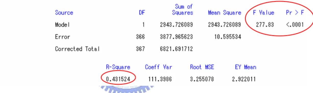
Lastly, we will utilize 1-way MANOVA to test the model validation. We will use 80/20 rules to classify the sample of customers into two kinds, where one kind of customer whose total number is only 20% of the entire sample but contributes toward 80% of total sales volumes. The two kinds of customers are named class 1 and 2 separately. We use class 1 & 2 as independent variables and use “the expected number of transactions”, “the expected active probability” and “the expected dollar volume spent per reorder” as dependent variables simultaneously to employ a 1-way MANOVA analysis. If we have statistical evidences to support the three dependent variables, it could explain the total variances a lot no matter if it’s collectively or individually. We will say with much confidence that “the expected number of transactions”, “the expected active probability” and “the expected dollar volume spent per reorder” could be treated as successful discrimination variables to differentiate customers and be a good starting point to achieve so called one-to-one marketing and implement other CRM strategies.

3.1 Assumptions 3.1.1 Terms Definition

(2) Each customer who is active is being termed as “Alive”, while each customer has left for any reason is being termed “Dead”.

(3) The observation time of each customer who is alive at time 0 is T.

(4) During the observation time “T”, each customer will have made X purchases and his last purchase will occur at tx, 0＜tx≦

T

.

(5) If a customer observed to have X purchases in a time period “T”, we could denote Zi as the dollar volume of per order i (i=1,…, X), and denote

as the average dollar volume spent by the customer.

(6) ρ is dented a reliability coefficient. While estimating the expected dollar volume of a customer, we could use it to represent our confidence in utilizing observed past order amount relative to relying on the population average order amount. If X=1, we useρ . If X 1,1

≧

we useρ . x

(7) Hence, the information on each customer contains 4 elements: Information = (X, tx, T, Zi ).

Within the 4 elements, we could also correspond the three basic CRM variables “Recency” (R), “Frequency” (F), “Monetary” (M) to tx, X, Zi

respectively.

3.1.2 Assumptions

There are seven assumptions in our framework. The first four are identical to the ones of the BG/NBD model and the last three are the same with the ones of the Extended SMC model.

(1) Transactions by active customers follow Poisson distribution

While active, the number of transactions X, made by each customer in time period of length t is a Poisson random variable with a purchase rate λ. It means that the time between transactions is distributed exponential with the

(

)

( ) 0 , ; ₁ 1 1 > ≥ = − − ₋ − − j j t t j j t e t t t f

λ

λ

λ j j

∑

= = X i i Z X Z 1 1

same purchase rate λ.

(2) Individual customer retention/dropout probability follows Geometric distribution

After any transaction, a customer could become inactive with a dropout rate p. So the point at which a customer becomes inactive follows a geometric distribution with dropout rate p.

(3) Heterogeneity in purchase rates λ which follows Gamma distribution

The purchase rate λ of different customers follows a gamma distribution across the population of customers with shape parameter γ and scale parameter α.

(4) Heterogeneity in dropout rates p which follows Beta distribution

The dropout rate p of different customers follows a beta distribution across the

population of customers with two parameters a and b.

(5) The dollar volume of per order (Zi) of individual customer follows Normal

distribution

Zi

～

N( θ, )

The set of Zi are i.i.d. normal random variables with mean θ and variance

2

W

σ

which represents the variance in the dollar volume spent across reorders for a customer and is constant across customers.

(6) Heterogeneity in average amount spent per order θ which follows Normal distribution 2 W

σ

(

)

(

1−

)

1, =1,2,3,... = − j p p n transactio jth after y immediatel inactive P j

(

,

)

_{( )}

, 0 1 > Γ = − − λ γ λ α α γ λ γ γ e λα f

(

)

(

₍

₎

)

, 0 1 , 1 , 1 1 ≤ ≤ − = − − p b a B p p b a p g b a

θ

～

N( , )

Mean θ is assumed to vary across customers according to a normal

distribution with mean and variance which represents the variance in average dollar volume spent across customers.

(7) Rates λ, p, and θ are independent from each other

The average amount spent per order θ, the purchase rate λ and the dropout rate p vary independently across customers.

3.2 Model Development for a Randomly Chosen Customer

3.2.1 Expected Number of Transactions

The expected number of transactions in the time period (T, T+t] for a randomly chosen individual with observed purchase behavior (X, tx, T)(The BG/NBD model, Equation (10))

(1) 3.2.2 Expected Active Probability

(1) The active probability at the individual level

For the case where purchases were made in the period (0, T], the probability that a customer with purchase behavior (X, tx, T), is still active at T,

conditional on λ and p, is simply the probability that he did not drop out at tx and made no purchases in (tx, T], divided by the probability of making no purchases in (0, T]. (The BG/NBD model, Appendix)

[ ]

θ

E

2 A

σ

[ ]

θ E 2 A

σ

( )

(

)

x x x x x t T x b a t T t x b a x b x F t T T a x b a b a T t x X t Y E + > + ⎟⎟ ⎠ ⎞ ⎜⎜ ⎝ ⎛ + + − + + ⎥ ⎥ ⎦ ⎤ ⎢ ⎢ ⎣ ⎡ ⎟ ⎠ ⎞ ⎜ ⎝ ⎛ + + − + + + + ⎟ ⎠ ⎞ ⎜ ⎝ ⎛ + + + − − − + + = = γ γ

α

α

δ

α

γ

α

α

α

γ

1 1 ; 1 ; , 1 1 1 , , , , , , 0 1 2

(

)

( ) ( x) x t T t T x

e

p

p

e

p

p

T

t

x

X

T

at

active

P

_{− −} − −

−

+

−

=

=

λ

λ _λ

)

1

(

)

1

(

,

,

,

,

₍₂₎

(2) For easily calculation, multiplying equation (2) by

[

[

_x

]

]

x t x x t x x

e

p

e

p

λ λ

λ

λ

− − − −

−

−

1 1

)

1

(

)

1

(

(3) The result is: (The BG/NBD model, Equation (A2))

P

(

active

at

T

X

x

t

T

p

) (

_L

_p

p

_X

_x

e

_t

_T

)

x T x x x

_,

_,

_,

)

1

(

,

,

,

,

=

−

=

=

−

λ

λ

λ

λ ₍₃₎

(4) As the purchase rate λ and dropout rate p are unobserved, we compute

for a randomly chosen customer by taking the

expectation of (3) over the distribution of λ and p, updated to take into account the information X=x, tx, T:

(

₍

)

_{) (}

₎

dp d T t x X b a p f p T t x X T at active P b a T t x X T at active P x x x λ α γ λ λ α γ , , , , , , , , , , , , , , , , , 1 0 0 = ⋅ = = =

∫ ∫

∞ (4) (5) By Bayes theorem, the joint posterior distribution of λ and p is given by

(

)

(

) (

) (

)

(

a bX x t T

)

L b a p g f T t x X p L T t x X b a p f x x x , , , , , , , , , , , , , , , , , = ⋅ ⋅ = = =

α

γ

α

γ

λ

λ

α

γ

λ

(5)

(6) Substituting equation (3) and (5) in (4), we get

(

) (

₎

T t x X b a L A b a T t x X T at active P x x , , , , , , , , , , , = = =

α

γ

α

γ

(6) where

(

)

(

) (

)

(

)

( )

( )(

(

)

)

x T x x T x b a B x b a B dp d b a p g f e p A + − ∞ + Γ + Γ + = − =

∫ ∫

γ γ λ

α

γ

α

γ

λ

α

γ

λ

λ

, , , , 1 1 0 0 (7)

(

active atT X x t T

)

P = , x,

3.2.3 Expected Dollar Volume per Reorder

Case 1: X=1 (The Extended SMC model, Equation (10), (11))

(8)

Where Case 2: X 1

≧

(The Extended SMC model, Equation (12), (13), (14))

(9) Where

∑

=

=

X i i

Z

X

Z

1

1

(

_W X

)

A A X 2 2 2

σ

σ

σ

ρ

+ =

[

]

[ ]

θ

σ

σ

σ

σ

σ

σ

θ

E X Z X X Z Z E W A A W A A X ⎟⎟ ⎠ ⎞ ⎜⎜ ⎝ ⎛ + + ⎟⎟ ⎠ ⎞ ⎜⎜ ⎝ ⎛ + = ₂ 2 _{2 2} 2 ₂ 1,..., 2 2 2 1 W A A

σ

σ

σ

ρ

+

=

[ ]

θ

Z

ρ

Z

(

ρ

)

E

[ ]

θ

E

₁

=

_{1 1}

+

1−

₁

4. Empirical Analysis

4.1 Data Description

The database applied is retrieved from an online CD/VCD retailer. This database consists of the purchase history that customers have made in the whole year of 2006. In this database, we have user IDs, the purchase date, dollar volume spent, ZIP codes, and order quantities of each purchase event. For utilizing our model, we only need the first three transaction records and importantly only choose the customers who have ever made purchases at the online retailer in the first quarter of 2006 to organize our dataset. In this way, we could have a data covering their initial (trial) and subsequent (repeat) purchases occasions for the period January 2006 through December 2006. After restructuring, we changed the dataset from covering 2856 to 1003 purchase events and the total number of customers was 368 in the end.

Although the information in this dataset is complete enough for us to utilize our model, we still need to reorganize the dataset into five columns which are ID, X, t_x, T, andZ _{. ID numbers could represent different customers. X is the total number of}

transactions made by each customer in the period April 2006 through December 2006. T represents the total observation time of each customer and it may be different between customers. As the BG/NBD model, we get the value of T by the equation “T =52-time of first purchase”. “52” means that we have 52 weeks in 2006. For example, if a customer made his first purchase in January 21, we could transform the date into “3/week” through dividing “21” by “7”. So the unit of T is 49 for this customer. However, the method to get t_x is a little complicate. In first, we also need to transform the date of the last purchase of a customer into Y with unit of a week. Then through the equation “t_x=T-(52-Y)” we could finally get the value t_x of the customer.Z _{represents the average dollar volume spent by a customer and}

we could easily use the “AVERAGE” function in Excel to get it. (If Xi=0, t_xi=0

Figure1. Screenshot of Excel Worksheet of Raw Data

4.2 Parameter Estimation

4.2.1 Transaction/Dropout Process

To estimate the four parameters γ, α, a, and b of the BG/NBD model, we use the method of maximum likelihood estimation (MLE). One of the biggest advantages of the BG/NBD model is that we could use an easy way to estimate parameters. As we mentioned in Introduction, the likelihood function of the BG/NBD model is:

(10) After rewriting the original function to have A1~A4 form the new equation, we

could easily code it in Excel by taking the “log” of the whole equation, adding the four elements as “ln(all)”, summing “ln(all)” of 368 customers, and using the “Linear Programmer” of the Solver tool in Microsoft Excel to get a constrained biggest “LL”. However, before using the “Linear Programmer”, we have to set the initial value of the four parameters as “1”. We then find the four parameters. The following figure shows the sheet of parameter estimation.

(

)

(

)

( )

( )(

(

)

)

(

( )

)

( )(

(

)

)

(

)

(

)

( )

( ) (

(

) (

)

)

x x x x x x x x x t x b a A T A x b a b x b b a A x A where A A A A t x b a B x b a B T x b a B x b a B T t x X b a L + + > + > + ⎟⎟ ⎠ ⎞ ⎜⎜ ⎝ ⎛ + ⎟ ⎠ ⎞ ⎜ ⎝ ⎛ + + = ⎟ ⎠ ⎞ ⎜ ⎝ ⎛ + = + + Γ Γ + Γ + Γ = Γ + Γ = + ⋅ ⋅ = + Γ + Γ − + + + + Γ + Γ + = = γ γ γ γ γ γ γ α α γ α γ δ α γ α γ δ α γ α γ α γ 1 1 , 1 , , , 1 , 1 , , , , , , , 4 3 ' 2 1 4 0 3 2 1 0

Figure2. Screenshot of Excel Worksheet of Parameter Estimation

We now decompose the equation of “ln(A_1)” for easy understanding.

Because

(

)

( )

γ α γ γ Γ + Γ = x A₁

, then the equation of log of A1 in cell F8 is:

(

)

[

(

)

]

[

( )

]

( )

(

$1 8

)

( )

$1 $1*

(

$2

)

ln ln ln 1 _ ln B LN B B GAMMALN B B GAMMALN x A + − + = + Γ − + Γ =

γ

γ

γ

α

(11) The second equation above shows the function we code in Microsoft Excel. Therefore, the model estimation results are shown in Table 2.

Table2. Model Estimation Results of Transaction/Dropout Process

γ

0.523

α

7.791

a 0.027

b 0.219

4.2.2 Transaction Dollar Volume

To estimate the three parametersσ ,W2 σ and E(θ) of the Extended SMC model, A2 we could also utilize Microsoft Excel to perform the work.

(1) 2 W σ Estimation We have denoted 2 W

σ as the variance in the dollar volume spent across reorders for a customer in Conceptual Framework. Thus, in order to

estimateσ , we should choose a pool of customers who have ever made at W2 least 2 repurchases in their observation time period and the sample size is 159. At first, we use the “VARP” function in Microsoft Excel to compute the variances of the dollar volume spent across reorders by each customer

respectively. Then we use X (the number of reorders) of each customer as the weighted values to compute the weighted averageσ . The value of the W2 weighted averageσ is 117789.9. W2 (2) 2 A σ Estimation The denotation of 2 A

σ is the variance in average dollar volume spent across customers (θ). Nevertheless, because the value of θ could not be observed, we have complication to compute σ directly. However, the total variance (A2 σ ) 2 in amount spent across both reorders and customers (which equals σ +W2 σ ) is A2 available and equals to 756038.6. We compute this value for the same 159 customers by using the recent dollar volume spent (the dollar volume of t_x ) by each customer. As a result, the value of σ is estimated as A2

756038.6-117789.9=638248.6. (3) E(θ) Estimation

E(θ) is denoted the expected value of θ which is assumed to vary across

customers according to a normal distribution. We use the “AVERAGE” function in Microsoft Excel to compute the expected value of Ziof the

customers (i=1~368). In the end, we use the “AVERAGE” function again and the value E(θ) is estimated as 614.10. We use the following table to show the values of the three parameters.

Table3. Model Estimation Results of Transaction Dollar Volume

2 W σ 117789.9 2 A σ 638248.6 E(θ) 614.10 4.3 Model Results

4.3.1 Expected Number of Reorders (Conditional Expectation)

The expected number of reorders is computed using Equation (1). However, there is a value created from a complex function we need to estimate. This complicated function is called the Gaussian hyper-geometric function. In Literature Review, we have briefly mentioned this kind of function. Usually, we could have two methods to compute this function. One is numerical integration and the other is the algorithms. We will choose the method of numerical integration to compute it as the authors of the BG/NBD model. Therefore, before forecasting the expected number of reorders, we will introduce this function simply and the process to estimates its value in Microsoft Excel.

(1) Gaussian hyper-geometric function₂F₁

( )

⋅ (Fader et al., 2005 b)

A. The prototype of 2

F

1

( )

⋅

where

( )

a _j is Pochhammer’s symbol, which denotes the ascending factoriala

(

a+1

) (

⋅ ⋅⋅ a+ j−1

)

. The series converges for z <1 and is divergent for

(

)

( ) ( )

_{( )}

( ) ( )

( )

!

,

...

2

,

1

,

0

,

!

;

;

,

1 2

j

z

c

b

a

u

where

u

c

j

z

c

b

a

z

c

b

a

F

j j j j j j j j j j j j

=

=

−

−

≠

=

∑

∑

∞ ∞

1 >

z ; if z =1, the series converges for c−b−a>0.

And we could have the following recursive expression for each term of the series:

where u₀ =1.

B. The Numerical Integration Method Employed in Microsoft Excel

It’s easy and simple for us to estimate2

F

1

( )

⋅

by utilizing the above series.

We just need to continue adding terms to the series untilujis less than “machine epsilon” (the smallest number that a specific computer recognizes as being bigger than zero). In Microsoft Excel, it’s easier to compute the series to a fixed number of terms, as a result, we will evaluate the first terms (j = 0, 1, 2…150).

In terminating the adding process of the series at j=150, whether have we evaluated too few terms? Because the speed with whichujÆ0 depends on the magnitude of z and the observed number of reorders X in Equation (1), where t T t z + + = α .

The only unfixed variable in Z is T (t = 52; α = 7.791). Under our dataset sampling rule, which is choosing the customers who have ever made their first purchase in the first quarter of 2006, the smallest T equals to 40.14. Thus the biggest z equals to 0.52. However, there is no point in going beyond

j = 40 for z<0.5 (Fader et al., 2005 b). As a result, based on the biggest z

value, it’s feasible for us to terminating the series at j = 150.

As to X, the biggest X in our dataset equals 50. We have tried to continue adding the terms to the biggest extent that j = 240, and we found the final result is the same as while j = 150.

(

)(

)

(

1

)

,

1

,

2

,

3

,...

1

1

1

=

−

+

−

+

−

+

=

−

j

z

j

j

c

j

b

j

a

u

u

j j

(2) Computing conditional expectation of number of reorders

After estimating the parameters and the value of2

F

1

( )

⋅

, we could also get

the conditional expectation of number of reorders in Microsoft Excel. Figure 3 shows the screenshot of excel worksheet of conditional expectation.

Figure3. Screenshot of Excel Worksheet of Conditional Expectation

In this worksheet, we first place the four model parameters we have

estimated in cells B1:B4. Then we place the purchase history

(

X =x,tx,T

)

of a

particular customer in cells B6:B9. For example, we choose the customer whose ID=34, X=20, tx=48.285 and T=49.142. For all customers, t equals to 52

because the length of time over which we wish to make the conditional forecast is a year. Furthermore, we use the method outlined above to compute₂F₁

( )

⋅

which is central to Equation (1). Corresponding to the prototype of₂F₁

( )

⋅ , the function parameters

(

a ,,b c

)

are given in cells E2:E4 and the function argument

( )

z are setting in cell E5. In last, we evaluate the first 151 terms of the series (cell E7:E157) and these terms are summed in cell E1. Then we could