Applicability of perturbative QCD and NLO power corrections for the pion form factor

共Received 4 September 2001; revised manuscript received 7 January 2002; published 19 March 2002兲

As is well recognized, the asymptotic of the perturbative QCD prediction for the pion form factor is much smaller than the upper end of the data. We investigate this problem. We first evaluate the next-to-leading-order

共NLO兲 power correction for the pion form factor. The corrected form factor contains nonperturbative

param-eters which are determined from a ␹2 fit to the data. Interpreting these parameters leads to the fact that the involved strong interaction coupling constant should be identified as an effective coupling constant under a nonperturbative QCD vacuum. If the scale associated with the effective coupling constant is identified as

具x典2_Q2_{, then Q}2_{, the momentum transfer square for the pion form factor to be measured, can have a value}

about 1 GeV2_{, and具x典, the averaged momentum fraction variable, can locate around 0.5. This circumstance}

is consistent with the asymptotic model for the pion wave function.

DOI: 10.1103/PhysRevD.65.074016 PACS number共s兲: 12.38.Bx, 13.40.Gp

I. INTRODUCTION

The exclusive process plays an important role in improv-ing our understandimprov-ing of strong interactions. A detailed analysis of the exclusive process may exhibit the constituents of hadrons and shed light on the underlying dynamics. One important progress in this respect is that perturbative QCD 共PQCD兲 was proposed for exclusive processes involving large momentum transfer关1–5兴. The basic idea of PQCD in these processes is the factorization theorem, which demon-strates that the transition amplitude can be factorized into a convolution of hadronic wave functions and a hard function. The hard function involving the short-distance interactions is perturbatively calculable, while the hadronic wave functions containing the long-distance physics are nonperturbative. PQCD has the ability to predict outcome due to the fact that for a specific hadron, its hadronic wave function is universal for transition processes in which the hadron can participate. The pion form factor has been investigated in the frame-work of PQCD关4–15兴. In the experimentally accessible en-ergy region of a few GeV2, the asymptotics of PQCD is only about one-fourth of the experimental value. This fact has received much attention in the literature. It also stimulated the debate about whether PQCD can be used for the pion form factor. As indicated by Isgur and Llewellyn 关16,17兴, most contributions to the form factor are from the soft end-point regions, i.e., the end-end-point singularity with which the perturbative calculation would become unreliable. To resolve this problem, Li and Sterman关6兴 proposed a modified hard-scattering approach for the hadronic form factor. In this ap-proach, the end-point singularity is replaced by a resumma-tion over soft radiative correcresumma-tions, i.e., the Sudakov form factor. It was found that, with the transverse degrees of free-dom playing the role of infrared cutoff, the PQCD contribu-tion becomes self-consistent for momentum transfer as low as a few GeV. Other approaches to solve the end-point sin-gularity problem have also been proposed, such as the trans-verse structure of the pion wave function关18–20兴, the effec-tive gluon mass 关21兴, and the frozen running coupling constant关22,23兴.

The discrepancy between theory and experiment may be

eliminated by power correction 关10–12,15兴 or radiative cor-rection. However, as shown in 关7,8兴, the next-leading-order 共NLO兲 radiative corrections can only contribute 20–30 %, which is still not enough to account for the data. Therefore, it is interesting to find out how large a contribution the NLO power correction can give. For the pion form factor, the NLO 关i.e., O(1/Q4_{)兴 power correction may receive contributions}

from operators composed either of one twist-2 and one twist-4 distribution amplitude共DA兲 or two twist-3 DAs 关24兴. The contributions from the latter have been calculated in PQCD 关10–12,15兴. To have a complete PQCD description for the form factor up to NLO power correction, the contri-butions from the former must also be considered. Based on the method developed in 关25兴, the former type of operator can be systematically calculated. The most important feature of this method is that the NLO power correction can have a partonic interpretation. By combining the contributions from both types of operators, we can find an interpretation for the data.

The organization of this paper is as follows. We investi-gate the power expansion for the␥*␲→␲process in Sec. II. The pion form factor F_␲(Q2) up to order O(Q⫺4) is evalu-ated in Sec. III. Using the pion form factor, we arrive at a phenomenological pion form factor by employing a least-␹2 fit to the data. Comparisons between the theoretical and the phenomenological pion form factors are given. Section IV contains discussions and conclusions.

II. COLLINEAR EXPANSION

In this section, we shall describe our approach for the power expansion for the ␥*␲→␲ process. The method we shall employ is called the collinear expansion 关25–27兴. Let ␴⫽␾*( P₂,k₂)丢␴p(k1,k2)丢␾( P1,k1) represent the

lowest-order amplitude for ␥*(q)␲( P1)→␲( P2) as

de-picted in Fig. 1共a兲. The explicit form for the amplitude␴ is expressed as ␴⫽

冕

d 4_k 1 共2␲兲4 d4k2 共2␲兲4Tr关␾*共k2兲␴p共k1,k2兲␾共k1兲兴, 共1兲

where␴p(k1,k2) denotes the amplitude for the partonic

sub-process, and␾(ki), i⫽1,2, represents the pion DAs. The丢 denotes convolution integrals over the loop momenta ki and traces over the color indices and the spin indices. To pick out the leading contribution, we assign the momenta of the initial- and final-state pions in the following way. We choose

P1⫽(P1⫹, P1⫺, P1_⬜)⫽(Q/

冑

2,0,0_⬜) and P2⫽(P2⫹, P2⫺, P2_⬜)

⫽(0,Q/

冑

2,0_⬜) such that PQCD is applicable for Q2⫽⫺q2 ⫽⫺(P2⫺P1)2 being large. We shall employ the light-cone

gauge in the following calculations. The internal loop mo-menta k_i␮, i⫽1,2, are parametrized as

k_i␮⫽xiPi␮⫹

k_i2⫹k_i2_⬜

2xi

n_i␮⫹k_i␮_⬜, 共2兲

where xi are dimensionless numbers of order unity and the vectors ni are in the direction of the opposite-moving exter-nal vectors such that ni•Pi⫽1, ni

2_{⫽0, n}

1•n2⫽2/Q2, and

also n1•P2⫽n2•P1⫽0. The first step is to perform a Taylor

expansion for the partonic amplitude

␴p共ki兲⫽␴¯p共ki⫽xiPi兲⫹共␴¯p兲␣共xi,xi兲wi␣⬘ ␣ _k

i

␣⬘_{⫹•••, 共3兲} where we have assumed the low-energy theorem

⳵

⳵k␣i␴p共ki兲

冏

k_i⫽x_iP_i ⫽共␴¯

p兲␣共xi,xi兲 共4兲 and have employed w_i␣_␣⬘k_i␣⬘⫽(ki⫺xiPi)␣ and wi␣⬘

␣ _⫽g ␣_⬘ ␣

⫺Pi␣ni␣⬘. The leading term ␾*丢␴¯p丢␾ contains leading, next-to-leading, and even higher-order power corrections which should be determined from the spin structure of ␴¯p, the term proportional to n”_ior P”_i. The n”_iterm would project a collinear qq¯ pair from the meson, while the P”iterm would not diminish only when the qq¯ pair carries noncollinear mo-menta. The second step is to substitute the leading partonic amplitude ␴¯p into the convolution integral with the pion wave function ␾ to factorize the leading and subleading power contributions,

␾*丢␴¯

p丢␾⫽␾0*丢␴¯p丢␾0⫹␾0*丢␴¯p丢␾1

⫹␾1*丢␴¯p丢␾0⫹•••, 共5兲

where␾0 and␾1 denote the leading twist共LT兲 and

next-to-leading twist共NLT兲 pion DAs, respectively. The␾₁ contains both short-distance and long-distance contributions. The short-distance contributions of ␾1 arise from the

noncol-linear components of ki. By the equation of motion, the noncollinear components of ki will induce one quark-gluon

vertex i␥_␣ and one special propagator in”_i/2x_i关27兴. Because the special propagator is not propagating on the light cone associated with the meson, the quark-gluon vertex and the special propagator should be incorporated into the hard func-tion, ␴¯p. In this way, ␾1 is factorized into ␾1

⬇(␾1

H

)_␣w₁␣_␣⬘(␾1,D)␣⬘and the short-distance piece (␾1

H )_␣ is absorbed into ␴¯p. This leads to the third step,

␾0*丢␴¯p丢␾1⫽␾0*丢␴¯p丢关共␾1 H_兲 ␣䊉w1␣⬘ ␣ _共␾ 1,D兲␣⬘兴 ⫽␾0*丢共␴¯p䊉␾1 H_兲 ␣丢w1␣⬘ ␣ _共␾ 1,D兲␣⬘, 共6兲

where (␾1,D)␣⬘ containing the covariant derivative D␣⬘

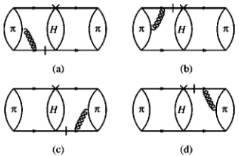
⫽i⳵␣⬘_⫺gA␣⬘_{is implied. The related Feynman diagrams for} this type of correction are displayed in Fig. 2. In these dia-grams, the quark propagator with one bar denotes the special propagator.

We now describe the final step of the collinear expansion. The second term of Eq. 共3兲 can contribute in subleading or-der of the power correction as it convolutes with ␾0. The

momentum factor k␣is absorbed by␾0 to become a

coordi-nate derivative, denoted as k␣␾0⬅␾1,␣⳵. Consider the other

contributions ␴1⬇␾0*丢(␴¯p)␣丢w1␣⬘

␣ _␾

1,A

␣_{⬘ from Fig. 1共b兲,}

where␾_1,A␣ contains gauge fields. Because of color and elec-tromagnetic gauge invariance, the diagrams from Fig. 3 are necessary. Note that the term w_1␣

⬘

␣ _A␣_{⬘appears automatically}

in the light-cone gauge. To arrive at a final result, some care should be taken. There are two kinds of contributions. The contributions of the first kind are from those diagrams in which the pion DAs contain the covariant derivative. We can set these as

FIG. 1. The leading diagrams for␥*␲→␲.

FIG. 2. The NLO power correction diagrams for␥*␲→␲. The

propagator with one bar means the special propagator.

FIG. 3. The other NLO power correction diagrams for ␥*␲

where we have employed ␾_1,␣_⳵⫹␾_1,A␣ ⫽␾_1,D␣ . The contribu-tions of the other kind are from those diagrams in which the DAs contain only gluon fields. Because of gauge invariance, the gluon fields need to be converted into field strengths. That is, we need to make the following substitution for the gluon field:

A␣→1 yG

␣␤_n

1␤, 共8兲

where the gluon field is associated with momentum y P1 and

the factor 1/y is then absorbed by the corresponding partonic amplitude (␴¯p)␣ such that (␴¯p)␣→(␴¯p

G₎

␣. These

contribu-tions are expressed as ␾0*丢共␴¯p G_兲 ␣丢w1␣⬘ ␣ _␾ 1,G ␣_⬘⬅␾ 0 *_丢共␴¯ p G_兲 1丢共␾1,G兲, 共9兲

where␾_1,G␣ means that it contains G␣␤. The last two steps of the collinear expansion can be applied for the final-state pion to calculate the other contributions. Finally, we write the am-plitude of the process ␥*␲→␲ under the collinear expan-sion up to O(1/Q4) as ␴0⫹␴1⬇␾0*丢␴¯p丢␾0 ⫹␾0*丢关␴¯p䊉␾1 H_⫹共␴¯ p兲1兴丢␾1,D ⫹␾1,D* 丢关共␾1* H_兲䊉 ␴ ¯ p⫹共␴¯p兲1*兴丢␾0⫹␾0*丢共␴¯p G_兲 1 丢␾1,G⫹␾1,G* 丢共␴¯p G_兲 1 *丢␾0. 共10兲

Where NLT DAs ␾1,D and ␾1,G are involved in the NLO

power correction.

The remaining tasks to be considered are the factoriza-tions of the spin indices, the color indices, and the momen-tum integrals over the loop partons. We refer the reader to 关25兴 for details of these factorizations. For factorization of spin indices, we employ the expansion of the meson DA into its spin components as

␾0,1⫽

兺

⌫ ␾0,1

⌫ _{⌫, 共11兲}

where⌫ denotes the Dirac matrix ⌫⫽1,␥␮,␥␮␥5,␴␮␯, and

␾1 represents␾1,D or ␾1,G. The choice of the lowest twist

components ␾0,1⌫ of ␾0,1can be made by employing power

counting 关25兴. For the factorization of the color indices, we employ the convention that the color indices of the parton amplitudes are extracted and attributed to the meson DAs. The factorization of the momentum integral is performed by making use of the fact that the leading parton amplitudes depend only on the momentum fraction variables xi. The momentum integrals are then converted into the integrals over fraction variables.

III. O„QÀ4… CONTRIBUTIONS

The amplitude for the ␥*␲→␲ process can be param-etrized in terms of the pion form factor,

A共␥*␲→␲兲⫽⫺ie_␲F_␲共Q2兲共P1␮⫹P2␮兲, 共12兲

where Q2⫽(P2⫺P1)2denotes the virtuality of the

off-mass-shell photon and e_␲ is the pion charge. The leading contri-bution of the pion form factor F_␲(Q2) is expressed as

F_␲LO共Q2兲⫽128␲␣s共Qeff 2 _兲 9Q2

冕

0 1 dx

冕

0 1 dy␾共x兲␾共y兲 x y . 共13兲

Applying␾(x)⫽3 f_␲x(1⫺x)/

冑

2 into Eq. 共13兲, one can get

F_␲LO共Q2_兲⫽16␲␣s共Qeff 2 _兲f

␲

2

Q2 , 共14兲

where f_␲⫽93 MeV will be used below in the numerical analysis.

We now describe the calculations of the NLO power cor-rection. We shall employ the light-cone gauge. The leading Feynman diagrams displayed in Fig. 4 are considered. After explicit evaluations for each diagram, we find the nonvanish-ing contribution is from Fig. 4共d兲. The result then reads

F_␲NLO共Q2兲⫽⫺256␲␣s共Qeff 2 _兲 9Q4 ⫻

冕

0 1 dx

冕

0 1 d y关G共x兲⫹G ˜_{共x兲兴␾共y兲} x2y ⫹共x↔y兲, 共15兲 where G(x) and G˜ (x) denote twist-4 pion DAs 关25兴. To simplify the situation further, we assume that G(x) and G˜ (x)

FIG. 4. The leading NLO power correction diagrams for␥*␲

contribute equally. A remark for the calculation is that we have employed the spin tensors i⑀_⬜␣␤␥_␤ for G(x) and

d_⬜␣␤␥_␤␥5 for G˜ (x), where ⑀_⬜␣␤⫽⑀␣␤␥␭P1␥n1␭ and d_⬜␣␤

⫽P1␣n1␤⫹n1␣P1␤⫺g␣␤.

We have employed the effective coupling ␣_s(Q_eff2 ) with the argument Q_eff2 ⬅

具

x y Q2

典

, where the brackets denote the average under a nonperturbative QCD vacuum. This is con-trary to the usual approach in PQCD, in which ␣_s(Q2_{) is}

taken to be running with Q2. The scale x y Q2of␣sis chosen as the momentum transfer of the exchanged gluon. From the factorization point of view, we may incorporate

具

x y Q2

典

into

具

x

典具

y

典

Q_fact2 by a factorization scale Qfact, which denotes a

scale to separate the perturbative and nonperturbative dy-namics. After substituting G(x)⫽3

冑

2␲2f_␲3x(1⫺x) 关25兴 and

evaluating the integrals, there still remains an infrared diver-gence关10,28兴 F_␲NLO共Q2兲⫽⫺512␲ 3_f ␲ 4_␣ s共Qeff 2 _兲 Q4

冉

冕

共1⫺x兲 x dx

冊

共16兲

which is from on-shell quark lines. This divergence cannot be completely resolved under perturbation theory. There re-quires a resummation over the soft divergences associated with the virtual quark lines. One also needs to introduce a jet function to absorb these divergences. We shall skip the de-tailed perturbative structure of these divergences关10–12,28兴. The initial function for such a jet function is nonperturbative. We denote the jet function as J(Q_eff2 ) and reset the NLO form factor as F_␲NLO共Q2兲⫽⫺512␲ 3_f ␲ 4_␣ s共Qeff 2 _兲J共Q eff 2 _兲 Q4 . 共17兲

Combining F_␲LO(Q2) and F_␲NLO(Q2), we obtain

F_␲共Q2_兲⫽16␲␣s共Qeff 2 _兲f ␲ 2 Q2

冉

1⫺ 32␲2_f ␲ 2_J共Q eff 2 _兲 Q2

冊

⫹O共Q⫺6_{兲. 共18兲}

Inspired by the above theoretical pion form factor, we can perform a least-␹2 _(␹

min

2 _{⫽7.967 42) fit to the data 关1–3兴 to}

obtain a phenomenological form factor,

F_␲fit共Q2兲⫽ A Q2

冉

1⫺

B

Q2

冊

, 共19兲

where A⫽0.468 95_{⫺0.043 29}⫹0.042 53 with 6␴ accuracy and B ⫽0.3009. The ␹2 _{analysis for the data is shown in Fig. 5. It}

is obvious that the data point at 10 GeV2 is the result of allowed errors. However, due to a small available range of

Q2 for the data, it is difficult to determine the asymptotic of the scaled form factor Q2F_␲(Q2) at large Q2. Comparing Eqs. 共18兲 and 共19兲, we are led to the following conclusions. 共i兲 The argument of ␣s(Q2) should be interpreted as an effective Q_eff2 ⬅

具

x

典

2_Q

fact

2 _{. That is, we need to take ␣}

s(Q2) as an effective coupling constant. The average fraction has the value

具

x

典

⬇0.57⫾0.03 for Qfact⫽1 GeV and ⌳QCD

⫽0.3 GeV. The values of

具

x

典

and Q_fact2 depend on the model for the pion DA关the asymptotic 共AS兲 model兴. If we perform a similar analysis by employing the Chernyak-Zhitnitsky 共CZ兲 model ␾(x)⫽15f_␲x(1⫺x)(1⫺2x)2/

冑

2 and G(x)⫽15

冑

2␲2f_␲3x(1⫺x)(1⫺2x)2 关25兴, we can

have Q_fact2 ⫽13.12_⫺3.39⫹5.79 GeV2 for

具

x

典

⬇0.5 or Q_fact2

⫽32.8_⫺8.5⫹14.5 _GeV2_for

_具

_x

_典

_{⬇0.1. It is clear that the CZ model}

is less consistent with PQCD than the AS model.

共ii兲 A less model-dependent property of the effective cou-pling constant can be described. The change in⌳_QCDwould affect the location of the average fraction variable

具

x

典

for a fixed factorization scale Qeff. On the other hand, for a fixed

具

x

典

, Qeff would vary with ⌳QCD. Nevertheless, there only

exist finite possible consistent solutions for⌳QCD, Qeff, and

具

x

典

.

FIG. 5. Plot of the least␹2_{fit共solid line兲 and}

C.L.⫽99.73% 共dash line兲 for Q2F_␲(Q2). The ex-perimental data are taken from关1–3兴.

共iii兲 The effective value of the J function at Qeff 2

is also model-dependent with a value of about 0.11 for the AS model and 0.026 for the CZ model.

共iv兲 Because the pion-photon transition form factor

F_␲␥(Q2) up to O(1/Q4) takes the form关25兴

F_␲␥共Q2兲⫽2 f␲ Q2

冉

1⫺

8␲2f_␲2

Q2

冊

, 共20兲

it is interesting to define the ratio R_␲ 关5兴,

R_␲I共Q2兲⫽ F␲ fit_共Q2_兲

4␲Q2F_␲␥2 共Q2兲, 共21兲

which has a theoretical expression valid for Q2⭓1 GeV2,

R_␲I共Q2兲⫽␣s共Qeff 2 _兲

冉

1⫹16␲ 2_f ␲ 2_{关1⫺2J共Q} eff 2 _兲兴 Q2 ⫺64␲ 4_f ␲ 4 Q4 ⫹O共1/Q 6_兲

冊

_{. 共22兲}

Comparing the prediction of F_␲␥ in Eq.共20兲 with the data 关29兴 gives␹2_{⫽12.8 for 15 data points. Note that the F}

␲␥in

Eq. 共20兲 is multiplied by 5/3 if the CZ model for the pion DAs has been employed. The ratio R_␲I is then smaller by 9/25. However, it has been shown关25兴 that the data 关29兴 for the F_␲␥form factor are more suited to the AS model than the CZ model, because the result with CZ DAs has␹2⫽390 共see the Fig. 3 in关25兴兲. Since Eq. 共20兲 is close to the experiment, we may take it as a fit to the data. The ratio R_␲I(Q2) is a ratio of observable over observable.

As the pion-photon transition form factor with the NLO correction, which has the expression

F_␲␥as 共Q2_兲⫽2 f␲ Q2

冉

1⫺ 5 3 ␣s共␮R 2_兲 ␲

冊

共23兲

with␮_R2⫽Q2/9, can also explain the data (␹2⫽57.8), we can define a similar ratio

R_␲II共Q2兲⫽ F␲ fit_共Q2_兲

4␲Q2_关F

␲␥

as_共Q2_兲兴2 共24兲

whose expression reads

R_␲II共Q2兲⫽␣s共Qeff 2 _兲

冉

1⫹10 3 ␣s共␮R 2_兲 ␲ ⫺ 25 9 ␣s 2_共␮ R 2_兲 ␲2 ⫺32␲ 2_f ␲ 2_J共Q eff 2 _兲 Q2 ⫹O共␣s 3_兲

冊

_{. 共25兲}

The F_␲␥as (Q2) in Eq.共23兲 is calculated by the AS model for the leading twist pion DA and the usual one-loop formula for the QCD running coupling constant,

␣s共Q2兲⫽ 4␲ ␤0ln Q2 ⌳QCD 2 , 共26兲

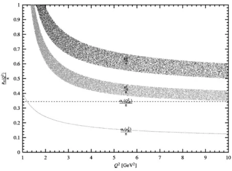
where⌳QCD⫽0.2 GeV and␤0⫽11⫺2/3nf with nf⫽2 have been used. We compare R_␲I(Q2)/␲and R_␲II(Q2)/␲ in Fig. 6. The errors for the ratios R_␲I(II) are from the errors associated with the fit pion form factor F_␲fit. Also plotted are␣s(Qeff

2 )/␲ and ␣s(␮R 2_{)/␲ employed in F} ␲␥ as _{. From Fig. 6, R} ␲ I(II) _are larger than␣s(␮R 2

) by about a factor of 3–5. The difference between R_␲ and␣s cannot be compensated for even by in-cluding the experimental errors for the F_␲␥ form factor, which can enlarge the error range for R_␲ by 100%. This seems to indicate that the other effects we have not consid-ered may be important. For example, we can encounter two possibilities: the NLO correction and the effects of QCD coupling in the low momentum region. The NLO correction can give contributions of at most 10% 关see point 共V兲兴. As for

FIG. 6. The comparisons between R_␲I/␲,

R_␲II/␲, ␣s(␮R

2

)/␲, and␣s(Qeff 2

the QCD coupling in the low momentum region, which can be modeled by an effective charge 关30兴,

␣V共Q2兲⫽ 4␲ ␤0 Q2⫹m_g2 ⌳V 2 共27兲

with nonperturbative parameters ⌳_V and m_g being a few

hundred MeVs, still cannot account for the large value of

R_␲. However, due to the low quality of the available data for the pion form factor, it is difficult to draw a firm conclusion regarding the above discrepancy between experiment and theory. We expect that future experiment could support fur-ther evidence to resolve the above problem.

共V兲 By taking into account the contributions from the

O(␣_s2) corrections to the leading twist pion form factor关31兴, Eq. 共18兲 is then modified as

F_␲共Q2兲⫽16␲␣s共Qeff 2 _兲f ␲ 2 Q2

再

1⫹ ␣s共Qeff 2 _兲 ␲

冋

␤0 4

冉

ln 1 18⫹ 14 3

冊

⫺3.92

册

冎

冉

1⫺ 32␲2f_␲2J共Q_eff2 兲 Q2

冊

⫹O共Q ⫺6_{兲. 共28兲}

The maximum values of the NLO ␣s corrections have been taken 关31兴. With the O(␣_s2) corrections, it only amounts to reinterpreting the scale Qeffinvolved in the coupling constant

␣s(Qeff 2

). The value of the jet function is unchanged. This can be seen from the expression of F_␲fit(Q2), where the ex-pansion is strictly ordered in 1/Q2. The analysis for Qeff is

close to that described in point 共i兲 within 5%. The O(␣_s2) correction for the ratio R_␲can also be considered by directly applying Eq. 共28兲. We find that the effects of the O(␣_s2) correction for R_␲are about 5–10 %. Of course, the complete

O(␣_s2) corrections are still not available. The analysis made here only reflects partial effects and seems too simple.

IV. DISCUSSIONS AND CONCLUSIONS

We now estimate the percentage of perturbation contribu-tions to the pion form factor. Our approach is to extend the analysis of Isgur et al. by including the NLO power correc-tion. The analysis of Isgur et al. estimates the perturbation contributions of the pion form factor by employing the frac-tional function f (⑀) f共⑀兲⫽

冕

0 1 dx

冕

0 1 d y␪共xy⫺⑀兲␾共x兲␾共y兲 xy . 共29兲

The parameter ⑀ describes a cutoff on xy in order to keep higher-twist contributions and higher-order effects at a rea-sonably small level. The reference scale is chosen at 1 GeV. Since f (⑀) is a mixture of perturbative and nonperturbative contributions, the perturbation parts are those corresponding to large values of x y Q2. For the AS model, f (⑀) reaches 90% for ⑀⫽1/150. This implies that the naive perturbative contribution is 90% accurate for Q2⫽150 GeV2. As for the pion form factor with NLO power corrections, the function

f (⑀) is modified, accordingly, as f共⑀NLO兲⫽

冕

0 1 dx

冕

0 1

dy␪共xy⫺⑀NLO兲␾共x兲␾共y兲

xy , 共30兲

where⑀NLO⫽⑀(1⫺c) with c⫽0.3009. It is easy to find that

f (⑀NLO) reaches 90% for ⑀NLO⫽1/150 or ⑀⫽1/105. This

means that the perturbative contribution with NLO power corrections is 90% accurate for Q2⫽105 GeV2. One may see that the inclusion of NLO power corrections can really improve the range of perturbation contributions by about 30%. As for the CZ model, the analysis can be made to reach a similar conclusion.

We now analyze the effects of the NLO power corrections from the operators composed in terms of two twist-3 pion DAs 关10–12,15兴. This type of NLO power correction takes the expression F_␲NLO共Q2兲⫽16␲␣s共Q 2_兲f ␲ 2 m_␲4 Q4m₀2 J 2_共Q2_{兲. 共31兲}

The function J(Q2) is the jet function as introduced before. The factor m_␲2/m0 relates to the quark condensate

具

0兩q¯q兩0

典

as

m_␲2 m0

⫽⫺ 2

f_␲2

具

0兩q¯q兩0

典

. 共32兲

Using the standard value of the quark condensate

具

0兩q¯q兩0

典

(1 GeV)⫽(⫺240 MeV)3, one has m_␲2/m₀ ⬇1.56 GeV in comparison with (16␲2_f

␲

2

)1/2⬇1.17 GeV. By substituting␣s(Q2) by␣s(Qeff

2

) and J(Q2) by J(Q_eff2 ) in Eq. 共31兲 and adding Eq. 共31兲 into Eq. 共18兲, we can arrive at

F_␲共Q2兲⫽ 16␲␣_s共Q_eff2 兲f_␲2 Q2

冉

1⫺ 32␲2_f ␲ 2 Q2 J共Qeff 2 _兲 ⫹ m␲ 4 Q2m0 2J 2_共Q eff 2 _兲

冊

⫹O共Q⫺6_{兲. 共33兲}

This implies that the value of the jet function, J(Q_eff2 ) ⬇0.124, is changed by about 10%. It is obvious that Eq. 共31兲 is as important as Eq. 共18兲.

associated Sudakov form factor behaves like exp

冋

⫺8CF ␤0 ln

冉

Q 2 ⌳2

冊

ln

冉

ln共Q2/⌳2兲 ln共k_⬜2/⌳2兲

冊

册

⫽

冉

⌳ 2 Q2

冊

(8C_F/␤₀)ln[ln(Q2/⌳2)/ln(k_⬜2/⌳2)] , 共34兲

where k_⬜ is the transverse momentum of the loop momen-tum and⌳ represents ⌳QCD, and we have used CF⫽43. It is seen that the Sudakov form factor at k_⬜⬇⌳, where the power expansion makes sense, decreases faster than any power suppression for Q2⬎⌳2. Therefore, the Q2 behavior of the pion form factor at moderate Q2 is mainly controlled by the power correction.

We have developed a power expansion scheme for ␥*␲ →␲. The NLO power correction to the pion form factor has been calculated. By employing the form of the pion form factor with NLO power correction, we then perform a least-␹2 _{analysis for the data to derive a phenomenological pion}

stant with a factorization scale equal to 1 GeV. In addition, the averaged fraction variable is located at 0.5 in agreement with the AS model for the pion DA. The CZ model fails to give a consistent explanation for the data, because its relative factorization scale is in the range of 3 –7 GeV.

From the results of this paper and 关25兴, we see that the power correction for exclusive processes is not negligible and requires detailed investigations. Over past decades, we have accumulated abundant data for exclusive processes. Most data are in the low-energy region, which is where the power correction plays an important role. The leading or the asymptotic contribution only gives information about the hadronic wave function, the static property of QCD, while the power correction can reveal the dynamics of QCD.

ACKNOWLEDGMENTS

This work was supported in part by the National Science Council of R.O.C. under Grant No. NSC89-2811-M-009-0024.

关1兴 C.J. Bebek et al., Phys. Rev. Lett. 37, 1525 共1976兲. 关2兴 C.J. Bebek et al., Phys. Rev. D 17, 1693 共1978兲.

关3兴 NA7 Collaboration, S.R. Amendolia et al., Nucl. Phys. B277,

168共1986兲.

关4兴 G.P. Lepage and S.J. Brodsky, Phys. Lett. 87B, 359 共1979兲. 关5兴 G.P. Lepage and S.J. Brodsky, Phys. Rev. D 22, 2157

共1980兲.

关6兴 H. Li and G. Sterman, Nucl. Phys. B381, 129 共1992兲. 关7兴 R.D. Field, R. Gupta, S. Otto, and L. Chang, Nucl. Phys.

B186, 429共1981兲.

关8兴 B. Melic, B. Nizic, and K. Passek, Phys. Rev. D 60, 074004 共1999兲.

关9兴 A.V. Efremov and A.V. Radyushkin, Phys. Lett. 94B, 245 共1980兲.

关10兴 B.V. Geshkenbein and M.V. Terentev, Phys. Lett. 117B, 243 共1982兲.

关11兴 B.V. Geshkenbein and M.V. Terentev, ITEP-45-1982. 关12兴 B.V. Geshkenbein and M.V. Terentev, Yad. Fiz. 40, 758 共1984兲

关Sov. J. Nucl. Phys. 40, 487 共1984兲兴.

关13兴 V.L. Chernyak and A.R. Zhitnitsky, Phys. Rep. 112, 173 共1984兲.

关14兴 R. Jakob and P. Kroll, Phys. Lett. B 315, 463 共1993兲; 319,

545共E兲 共1993兲.

关15兴 F. Cao, Y. Dai, and C. Huang, Eur. Phys. J. C 11, 501 共1999兲.

关16兴 N. Isgur and C.H. Llewellyn Smith, Phys. Rev. Lett. 52, 1080 共1984兲.

关17兴 N. Isgur and C.H. Llewellyn Smith, Nucl. Phys. B317, 526 共1989兲.

关18兴 T. Huang and Q.X. Shen, Z. Phys. C 50, 139 共1991兲. 关19兴 Z. Dziembowski and L. Mankiewicz, Phys. Rev. Lett. 58, 2175

共1987兲.

关20兴 F.G. Cao, T. Huang, and B.Q. Ma, Phys. Rev. D 53, 6582 共1996兲.

关21兴 C.R. Ji, A.F. Sill, and R.M. Lombard, Phys. Rev. D 36, 165 共1987兲.

关22兴 C.R. Ji and F. Amiri, Phys. Rev. D 42, 3764 共1990兲. 关23兴 J.M. Cornwall, Phys. Rev. D 26, 1453 共1982兲.

关24兴 V.M. Braun, A. Khodjamirian, and M. Maul, Phys. Rev. D 61,

073004共2000兲.

关25兴 T. Yeh, hep-ph/0107018.

关26兴 R.K. Ellis, W. Furmanski, and R. Petronzio, Nucl. Phys. B207,

1共1982兲.

关27兴 J. Qiu, Phys. Rev. D 42, 30 共1990兲. 关28兴 H. Li, hep-ph/0102013.

关29兴 CLEO Collaboration, J. Gronberg et al., Phys. Rev. D 57, 33 共1998兲.

关30兴 S.J. Brodsky, C.R. Ji, A. Pang, and D.G. Robertson, Phys. Rev.

D 57, 245共1998兲.