Dynamics of phytoplankton community under photoinhibition
Sze-Bi Hsua,b,, Chiu-Ju Linb, Chih-Hao Hsiehc, Kohei Yoshiyamad
aNational Center for Theoretical Sciences, Hsinchu 300, Taiwan
bDepartment of Mathematics, National Tsing-Hua University, Hsinchu 300, Taiwan cInstitute of Oceanography and Institute of Ecology and Evolutionary Biology, National Taiwan
University, Taipei, 10617, Taiwan
dRiver Basin Research Center, Gifu University, Gifu 501-1193, Japan
Abstract
We analyzed a model of phytoplankton competition for light in a well-mixed water column. The model, proposed by Gerla et al. (2011), assumed inhibition of phytoplankton growth at high irradiance (photoinhibition). We described the global behavior through mathemat-ical analyses, providing a general solution to the multi-species competition for light with photoinhibition. We classified outcomes of 2- and 3-species competitions as examples, and evaluated feasibility of the theoretical predictions using published growth-irradiance relation-ships. Our results suggested that photoinhibition does not play a major role in organizing phytoplankton communities as long as we consider light utilization traits obtained in culture growth conditions.
Keywords: competition for light, photoinhibition, Allee effect, competitive facilitation, alternative stable states
1. Introduction
Light is an essential resource for photosynthesis and driving energy of terrestrial and aquatic ecosystems. The excess energy, on the other hand, causes damages to the pho-tosynthetic machinery, and thereby lessens phopho-tosynthetic production. This phenomenon, known as photoinhibition, is prevalent to all photosynthetic organisms from cyanobacteria to higher plants. The molecular mechanisms have been investigated intensively [28], and unimodal photosynthesis and irradiance (p-I) relationships of algal species were observed in laboratories [12]. The corresponding theoretical frameworks were proposed [8, 32, 11, 23], which are in good agreement with measured p-I relationships. Field observations showed impacts of photoinhibition on ecosystem-level properties such as the magnitude and spatial variations of primary productivity in aquatic ecosystems [1, 3, 4, 5, 9, 24]. However, in-fluences of photoinhibition on ecological community structure are rarely investigated both empirically and theoretically.
One exception is Gerla et al. [10], where they extended the classical light competition model of phytoplankton [14, 29] by including the effect of photoinhibition (see also [13]).
Email addresses: [email protected] (Sze-Bi Hsu), [email protected] (Chiu-Ju Lin), [email protected] (Chih-Hao Hsieh), [email protected] (Kohei Yoshiyama)
Their results suggested that phytoplankton population may exhibit a strong Allee effect and competitive facilitation. A strong Allee effect is a phenomenon that population goes extinct when the density is below a threshold, while it persists when the density is above the threshold. Competitive facilitation is a phenomenon that a species that cannot grow in monoculture can grow and take over the community under the presence of another species. Their theory and predictions, based on previous results of Huisman and Weissing [14, 29] and graphical approach, indicated significance of photoinhibition in shaping phytoplankton community structure.
In this paper, we aim at analyzing the global dynamical behavior of a phytoplankton competition model with photoinhibition proposed by Gerla et al [10], and at evaluating fea-sibility of the theoretical predictions using empirical growth-irradiance (g-I) curves compiled by [26]. In doing so, we supplement the theory of [10], and shed light on difficulties and challenges in trait-based approaches for elucidating the phytoplankton community structure in nature.
2. The model and main results
Consider a model of n phytoplankton species competing for light in a well-mixed water column. The depth of the water column z ranges from 0 (the water surface) to zmax (the
bottom of the water column). Let xi(t) be the population density of the i-th species per unit surface of water at time t. The governing equation for the i-th species takes the form: (See [10], [29]) dxi dt = ( 1 zmax ∫ zmax 0 pi(I(z, t))dz− di ) xi, i = 1, 2, ..., n. (1)
The first term within the parentheses denotes growth rate averaged vertically in the water column, where pi(I) is the specific growth rate as a function of light I(z, t). The second term di denotes the specific loss rate.
According to Lambert-Beer’s law, the light intensity at depth z and time t is expressed by I(z, t) = Iinexp −∑n j=1 kjxj(t) z zmax − K bgz ,
where Iin is the incident light intensity at the top of the water column, kj, the specific light attenuation coefficient of j-th species, and Kbg, the background light attenuation coefficient.
Following [14, 29], we define Ioutto be the light intensity at the bottom of the water column
Iout(t) = I(zmax, t) = Iinexp
−∑n j=1 kjxj(t)− Kbgzmax . (2)
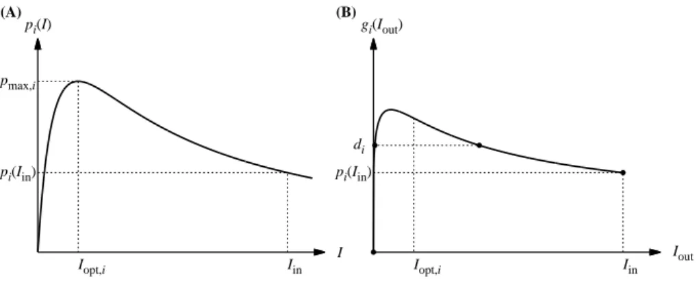
The specific growth rate pi(I) decays when the light is too strong, known as photoinhi-bition [26]. General assumptions of such function are: pi(I)≥ 0 and dp/dI < ∞ for I > 0,
(A) pi(I) Iin I Iopt,i pi(Iin) pmax,i (B) gi(Iout) Iin Iout Iopt,i pi(Iin) di
Figure 1: (A) Growth rate pi(I) of species i as a function of irradiance I expressed by eq. (3). The curve has a peak at the optimal irradiance Iopt,i with the maximum growth rate pmax,i. (B) The corresponding
growth rate averaged over the water column gi(Iout) as a function of Iout, irradiance at the bottom of the
water column. Mathematical analysis shows gi(0) = 0, gi(Iin) = pi(Iin), and that the curve has a peak at Ioutwhich is lower than Iopt,i. When the loss rate diis lower than the maximum of gi, there are λiand µi
such that gi(λi) = gi(µi) = di.
pi(0) = 0, and
dpi
dI > 0 for 0≤ I < Iopt,i dpi
dI < 0 for I > Iopt,i
where Iopt,iis the light intensity that attains the maximum specific growth rate. A commonly
used example of functions that satisfy the above conditions is (Fig. 1A):
pi(I) = pmax,iI pmax,i αiIopt,i2 I2+(1− 2 pmax,i αiIopt,i ) I +pmax,i αi , (3)
where pmax,i is the maximum growth rate and αi is the initial slope of pi(I). According to [10], the averaged growth rate in (1) can be rewritten as:
1 zmax ∫ zmax 0 pi(I(z, t))dz = 1 ln Iin− ln Iout ∫ Iin Iout pi(I) I dI. (4)
We define the right-hand side of (4) to be gi(Iout), and the governing equation (1) becomes dxi
dt = [gi(Iout(t))− di]xi, i = 1, 2, ..., n. (5) The function gi(Iout) satisfies gi(0) = 0, gi(Iin) = pi(Iin). When Iin > Iopt, gi(Iout) is a
unimodal function. In addition, when di is less than the maximum of gi(Iout), there are two
points Iout = λi, µi such that: gi(λi) = gi(µi) = di; gi(Iout) > di for Iout ∈ (λi, µi); and gi(Iout) < di for Iout∈ [0, λi)∪ (µi,∞) (Fig. 1B; see Appendix for the proof).
We define I0:= Iine−Kbgzmax, and then (2) is rewritten as: Iout(t) = I0exp −∑n j=1 kjxj(t) . (6)
We study (5) where Iout(t) is defined in (6) with the initial condition: xi(0) > 0 for i = 1, 2, .., n.
From the mathematical analysis, we prove that the solutions are positive and bounded, and that if λi > I0, then the species i goes to extinct as time t becomes large (See Appendix).
From now on, we simply assume
0 < λ1< λ2< ... < λn< I0,
and µi̸= µj, λj, I0for i̸= j.
First we consider steady state of (5) and the local property. Steady state can be classified into three types:
E0= (0, 0, ..., 0);
Eλr = (0, ..., 0, xλr, 0, ..., 0), r = 1, 2, ..., n;
Eµr = (0, ..., 0, xµr, 0, ..., 0) for which r satisfies µr< I0,
where xλr and xµr are expressed by:
xλr = ln I0− ln λr kr xµr = ln I0− ln µr kr . For mathematical convenience, we introduce a positive cone
Ω :={(x1, x2, ..., xn)∈ Rn: xi> 0, i = 1, 2, ..., n.} and set S as S := n ∪ i=1 (λi, µi).
For some species i and j, intervals (λi, µi) and (λj, µj) may overlap. For example, if λi< λj and µi < µj, the union will be (λi, µj). In a similar manner, S is expressed as a disjoint union of several connected components:
S = (λp1, µq1)∪ (λp2, µq2)∪ ... ∪ (λpm, µqm),
where m is the number of connected components, and λpj and µqj, respectively, are the left
and right endpoints of component j (j = 1, 2, . . . , m). In addition, we introduce two sets of steady state, SL and SR:
SL={Eλr : λr is a left endpoint of components of S} ∪ {E0} if I0̸∈ S, SR={Eµr : µr is a right endpoint of components of S}.
From linearization at steady state and the stability analysis, we can conclude that the local property is related to the structure of S (See Appendix). The results are summarized as: steady state E∈ SL is locally stable; E ∈ SR is saddle with (n− 1)-dimensional stable manifold (denoted by Ws(E) for E ∈ SR), which intersects Ω; and other steady states are unstable, some of which are saddle with a stable manifold which does not intersect Ω.
By using mathematical methods similar to [7], we prove that Iout(t) converges as t goes
to infinity. Based on the result and local stability of steady state, we can describe the global behavior of system (5).
Theorem 1. All solutions with initial condition in Ω\ (∪E∈SRWs(E)) satisfy lim
t→∞(x1(t), x2(t), ..., xn(t)) = E∈ SL, and the outcome depends on initial condition.
Theorem 1 tells us that all solutions from a positive initial condition converge to a steady state in the set SLexcept when the initial condition lies in the stable manifold Ws(E) with E ∈ SR. The positive cone Ω is divided by ∪E∈SRWs(E) into several regions, and there is only one locally stable steady state E ∈ SL in each region that attracts all solutions with the initial condition in this region. These statements completely describe the global dynamics of the system investigated by [10], and assure that the competition outcomes can be evaluated from the structure of S and the position of I0 for any number of species. We
shall investigate some examples in next section.
3. Feasibility of theoretical predictions
Gerla et al. [10] showed diverse outcomes of 2-species competition including strong Allee effect, competitive facilitation, and multiple positive alternative stable states. In this section, we demonstrate how mathematical properties of the system can be translated to ecological phenomena in 2- and 3-species competitions. Then we test feasibility of the theoretical predictions by applying empirical g-I curves to the model.
In order to classify competition outcomes, we suppose our basic assumption λi < I0
holds for all species. Mathematical properties include the structure of S and the position of I0 relative to S, the set of stable steady states, and the set of saddle with the stable
manifold in Ω. The corresponding ecological phenomena include a strong Allee effect (AL), competitive facilitation (FA), and presence of positive alternative stable states (ASS+). FA is distinguished by the case when an interval of positive growth of a winning species overlaps, but does not completely cover, that of other species. In FA, a winning species i cannot persist in the system for some Iout where a losing species j can. As species j grows in the system
and reduce Iout, species i eventually takes over the system. This case is described by j→ i
in tables. In 3-species competition, stable steady state may be achieved through a sequence of competitive facilitation such as: 3→ 2 → 1.
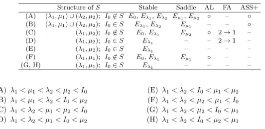
Table 1: Mathematical properties and ecological phenomena for the eight possible cases of 2-species compe-tition. Mathematical properties shown in the table include structure of set S and the position of I0relative
to S (Structure of S), set of stable steady states (Stable), and set of saddles with the stable manifold in Ω (Saddle). Ecological properties include a strong Allee effect (AL), competitive facilitation (FA), and presence of positive alternative stable states (ASS+).
Structure of S Stable Saddle AL FA ASS+
(A) (λ1, µ1)∪ (λ2, µ2); I0̸∈ S E0, Eλ1, Eλ2 Eµ1, Eµ2 ◦ – ◦ (B) (λ1, µ1)∪ (λ2, µ2); I0∈ S Eλ1, Eλ2 Eµ1 – – ◦ (C) (λ1, µ2); I0̸∈ S E0, Eλ1 Eµ2 ◦ 2 → 1 – (D) (λ1, µ2); I0∈ S Eλ1 – – 2→ 1 – (E) (λ1, µ2); I0∈ S Eλ1 – – – – (F) (λ1, µ1); I0̸∈ S E0, Eλ1 Eµ1 ◦ – – (G, H) (λ1, µ1); I0∈ S Eλ1 – – – – (A) λ1< µ1< λ2< µ2< I0 (B) λ1< µ1< λ2< I0< µ2 (C) λ1< λ2< µ1< µ2< I0 (D) λ1< λ2< µ1< I0< µ2 (E) λ1< λ2< I0< µ1< µ2 (F) λ1< λ2< µ2< µ1< I0 (G) λ1< λ2< µ2< I0< µ1 (H) λ1< λ2< I0< µ2< µ1
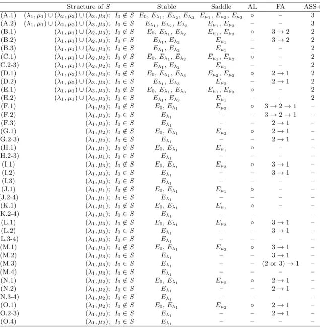
Mathematical properties and the corresponding ecological phenomena for 2-species com-petitions are summarized in Table 1. Based on backward trajectory and Theorem 1, we can describe the global behavior of the solutions of system (5) (Fig. 2). Note that the case (A) is equivalent to the intriguing case discussed in Fig. 6 of Gerla et al [10], where both species go extinct when they are initially abundant in the system (Fig. 2A).
For 3-species competition, we have the following 48 cases: (A.1) λ1< µ1< λ2< µ2< λ3< µ3< I0 (A.2) λ1< µ1< λ2< µ2< λ3< I0< µ3 (B.1) λ1< µ1< λ2< λ3< µ2< µ3< I0 (B.2) λ1< µ1< λ2< λ3< µ2< I0< µ3 (B.3) λ1< µ1< λ2< λ3< I0< µ2< µ3 (C.1) λ1< µ1< λ2< λ3< µ3< µ2< I0 (C.2) λ1< µ1< λ2< λ3< µ3< I0< µ2 (C.3) λ1< µ1< λ2< λ3< I0< µ3< µ2 (D.1) λ1< λ2< µ1< µ2< λ3< µ3< I0 (D.2) λ1< λ2< µ1< µ2< λ3< I0< µ3 (E.1) λ1< λ2< µ2< µ1< λ3< µ3< I0 (E.2) λ1< λ2< µ2< µ1< λ3< I0< µ3 (F.1) λ1< λ2< µ1< λ3< µ2< µ3< I0 (F.2) λ1< λ2< µ1< λ3< µ2< I0< µ3 (F.3) λ1< λ2< µ1< λ3< I0< µ2< µ3 (G.1) λ1< λ2< µ1< λ3< µ3< µ2< I0 (G.2) λ1< λ2< µ1< λ3< µ3< I0< µ2 (G.3) λ1< λ2< µ1< λ3< I0< µ3< µ2 (H.1) λ1< λ2< µ2< λ3< µ3< µ1< I0 (H.2) λ1< λ2< µ2< λ3< µ3< I0< µ1 (H.3) λ1< λ2< µ2< λ3< I0< µ3< µ1 (I.1) λ1< λ2< µ2< λ3< µ1< µ3< I0 (I.2) λ1< λ2< µ2< λ3< µ1< I0< µ3 (I.3) λ1< λ2< µ2< λ3< I0< µ1< µ3 (J.1) λ1< λ2< λ3< µ3< µ2< µ1< I0 (J.2) λ1< λ2< λ3< µ3< µ2< I0< µ1 (J.3) λ1< λ2< λ3< µ3< I0< µ2< µ1 (J.4) λ1< λ2< λ3< I0< µ3< µ2< µ1 (K.1) λ1< λ2< λ3< µ2< µ3< µ1< I0 (K.2) λ1< λ2< λ3< µ2< µ3< I0< µ1 (K.3) λ1< λ2< λ3< µ2< I0< µ3< µ1 (K.4) λ1< λ2< λ3< I0< µ2< µ3< µ1 (L.1) λ1< λ2< λ3< µ2< µ1< µ3< I0 (L.2) λ1< λ2< λ3< µ2< µ1< I0< µ3 (L.3) λ1< λ2< λ3< µ2< I0< µ1< µ3 (L.4) λ1< λ2< λ3< I0< µ2< µ1< µ3 (M.1) λ1< λ2< λ3< µ1< µ2< µ3< I0
(M.2) λ1< λ2< λ3< µ1< µ2< I0< µ3 (M.3) λ1< λ2< λ3< µ1< I0< µ2< µ3 (M.4) λ1< λ2< λ3< I0< µ2< µ1< µ3 (N.1) λ1< λ2< λ3< µ3< µ1< µ2< I0 (N.2) λ1< λ2< λ3< µ3< µ1< I0< µ2 (N.3) λ1< λ2< λ3< µ3< I0< µ1< µ2 (N.4) λ1< λ2< λ3< I0< µ3< µ1< µ2 (O.1) λ1< λ2< λ3< µ1< µ3< µ2< I0 (O.2) λ1< λ2< λ3< µ1< µ3< I0< µ2 (O.3) λ1< λ2< λ3< µ1< I0< µ3< µ2 (O.4) λ1< λ2< λ3< I0< µ1< µ3< µ2
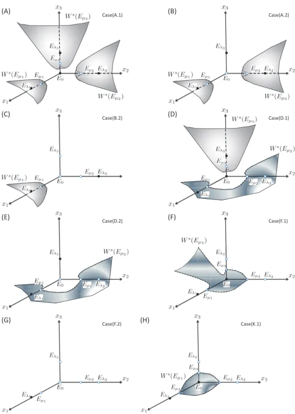
Mathematical properties and the corresponding ecological phenomena for 3-species com-petitions are summarized in Table 2. Based on the mathematical analysis, we can exactly describe the global behavior. We will not present each of 48 cases, but classify all cases by the number of attractor and the structure of stable manifold of saddle in Ω, resulting in 8 classical types (Fig. 3).
As we have seen in 2- and 3-species cases, the light competition model with photoin-hibition shows a variety of dynamical behavior. In order to evaluate feasibility of these theoretical predictions, we applied empirical g-I curves to the model. In [26], Schwaderer et al. compiled empirical data of g-I relationships of phytoplankton, and obtained g-I curves for 56 species. Among them, g-I relationships of 39 species indicated photoinhibition, and were expressed by eq. (3). Here we considered these 39 species for our numerical exper-iments. We used g-I curves instead of p-I curves because photosynthesis rates (carbon uptake per chlorophyll a) need to be multiplied by chlorophyll a to carbon ratio in order to obtain growth rate. Parameters of g-I curves ranged: the maximum growth rate pmax,i
(d−1), from 0.09 to 2.48 with the median 0.64; the initial slope αi (µmol photon−1 m2 s d−1), from 0.003 to 0.099 with the median 0.015; and the optimal irradiance Iopt,i (µmol
photon m−2 s−1), from 37.5 to 250.8 with the median 161.5. In numerical experiments, we set model parameters to combinations of low or high loss rate (di = 0.25, 0.5 [d−1]), and low, high, or a range of incident light (Iin= 500, 1000, 0–1000 [µmol photon m−2 s−1]) in
a clear (Kbg= 0.2 [m−1]) and shallow (zmax= 1 [m]) water column.
Positive growth intervals (λi, µi) are computed for the 39 species. Several species cannot grow for any Iout at d = 0.25 due to the low pmax,i (Figs. 4AB). Positive growth intervals
of two species (Scenedesmus crassus and Chlorella pyrenoidosa) ranged from < 10−4 to Iin
due to the high pmax,i (1.29 and 2.48) and the relatively high αi (0.042 and 0.045). Among species that can grow for some Iout, several species showed a strong Allee effect at d = 0.25
and Iin= 500 (Fig. 4A). On the other hand, most species showed a strong Allee effect (Figs.
4BCD) at high loss rate d = 0.5 and/or high incoming light Iin= 1000,
Figure 5 shows feasibility of theoretical predictions along the gradient of incoming light Iinwith an increment ∆Iin= 1. In monoculture, species either goes extinct, persists
regard-less of the initial condition, or shows a strong Allee effect (Figs 5AB). The number of the persistent species has a peak around the median of Iopt, and the number of species that show
a strong Allee effect increases with increasing Iin. The trends are similar for d = 0.25 and d = 0.5. In 2- and 3-species competition, we consider combinations of species that have a positive growth interval in monoculture for each Iin. For 2-species competition, we classified
the competition outcomes as in the Table 1. For 3-species competition, FA is distinguished whether 1 or 2 species play roles in facilitation (FA(1) and FA(2)), and ASS+, by the number of positive stable states (ASS+(2) and ASS+(3)). The number of combinations relative to the total was computed for each case of competition outcomes. When d = 0.25, the relative number of combinations that indicated FA and AL showed increasing trends with Iin while
Table 2: Mathematical properties and ecological phenomena for all possible cases of 3-species competition. Notation follows Table 1. ASS+ is distinguished by the number of positive stable states.
Structure of S Stable Saddle AL FA ASS+
(A.1) (λ1, µ1)∪ (λ2, µ2)∪ (λ3, µ3); I0̸∈ S E0, Eλ1, Eλ2, Eλ3 Eµ1, Eµ2, Eµ3 ◦ – 3 (A.2) (λ1, µ1)∪ (λ2, µ2)∪ (λ3, µ3); I0∈ S Eλ1, Eλ2, Eλ3 Eµ1, Eµ2 – – 3 (B.1) (λ1, µ1)∪ (λ2, µ3); I0̸∈ S E0, Eλ1, Eλ2 Eµ1, Eµ3 ◦ 3→ 2 2 (B.2) (λ1, µ1)∪ (λ2, µ3); I0∈ S Eλ1, Eλ2 Eµ1 – 3→ 2 2 (B.3) (λ1, µ1)∪ (λ2, µ3); I0∈ S Eλ1, Eλ2 Eµ1 – – 2 (C.1) (λ1, µ1)∪ (λ2, µ2); I0̸∈ S E0, Eλ1, Eλ2 Eµ1, Eµ2 ◦ – 2 (C.2-3) (λ1, µ1)∪ (λ2, µ2); I0∈ S Eλ1, Eλ2 Eµ1 – – 2 (D.1) (λ1, µ2)∪ (λ3, µ3); I0̸∈ S E0, Eλ1, Eλ3 Eµ2, Eµ3 ◦ 2→ 1 2 (D.2) (λ1, µ2)∪ (λ3, µ3); I0∈ S Eλ1, Eλ3 Eµ2 – 2→ 1 2 (E.1) (λ1, µ1)∪ (λ3, µ3); I0̸∈ S E0, Eλ1, Eλ3 Eµ1, Eµ3 ◦ – 2 (E.2) (λ1, µ1)∪ (λ3, µ3); I0∈ S Eλ1, Eλ3 Eµ1 – – 2 (F.1) (λ1, µ3); I0̸∈ S E0, Eλ1 Eµ3 ◦ 3→ 2 → 1 – (F.2) (λ1, µ3); I0∈ S Eλ1 – – 3→ 2 → 1 – (F.3) (λ1, µ3); I0∈ S Eλ1 – – 2→ 1 – (G.1) (λ1, µ2); I0̸∈ S E0, Eλ1 Eµ2 ◦ 2→ 1 – (G.2-3) (λ1, µ2); I0∈ S Eλ1 – – 2→ 1 – (H.1) (λ1, µ1); I0̸∈ S E0, Eλ1 Eµ1 ◦ – – (H.2-3) (λ1, µ1); I0∈ S Eλ1 – – – – (I.1) (λ1, µ3); I0̸∈ S E0, Eλ1 Eµ3 ◦ 3→ 1 – (I.2) (λ1, µ3); I0∈ S Eλ1 – – 3→ 1 – (I.3) (λ1, µ3); I0∈ S Eλ1 – – – – (J.1) (λ1, µ1); I0̸∈ S E0, Eλ1 Eµ1 ◦ – – (J.2-4) (λ1, µ1); I0∈ S Eλ1 – – – – (K.1) (λ1, µ1); I0̸∈ S E0, Eλ1 Eµ1 ◦ – – (K.2-4) (λ1, µ1); I0∈ S Eλ1 – – – – (L.1) (λ1, µ3); I0̸∈ S E0, Eλ1 Eµ3 ◦ 3→ 1 – (L.2) (λ1, µ3); I0∈ S Eλ1 – – 3→ 1 – (L.3-4) (λ1, µ3); I0∈ S Eλ1 – – – – (M.1) (λ1, µ3); I0̸∈ S E0, Eλ1 Eµ3 ◦ 3→ 1 – (M.2) (λ1, µ3); I0∈ S Eλ1 – – 3→ 1 – (M.3) (λ1, µ3); I0∈ S Eλ1 – – (2 or 3)→ 1 – (M.4) (λ1, µ3); I0∈ S Eλ1 – – – – (N.1) (λ1, µ2); I0̸∈ S E0, Eλ1 Eµ2 ◦ 2→ 1 – (N.2) (λ1, µ2); I0∈ S Eλ1 – – 2→ 1 – (N.3-4) (λ1, µ2); I0∈ S Eλ1 – – – – (O.1) (λ1, µ2); I0̸∈ S E0, Eλ1 Eµ2 ◦ 2→ 1 – (O.2-3) (λ1, µ2); I0∈ S Eλ1 – – 2→ 1 – (O.4) (λ1, µ2); I0∈ S Eλ1 – – – –
ASS+ were not observed in both 2- and 3-species competitions (Figs. 5CE). When d = 0.5, FA and AL showed similar increasing trends, and ASS+ was observed in a few combinations (Figs. 5DF). For 3-species competition, 3 positive alternative stable states ASS+(3) and sequential facilitation FA(2) were also possible in several combinations.
Overall, our numerical experiments indicated that ecological phenomena specific to the light competition model with photoinhibition were not common and occur in limited cases. A strong Allee effect was observed in <20% in monoculture (Figs. 5AB), <10% in 2-species competition (Figs. 5CD), and <1% in 3-species competition (Figs. 5EF). Competitive facilitation was observed in <10% in 2- and 3-species competition (Figs. 5CDEF). Positive alternative stable states were not observed except for very limited combinations (Figs. 5DF). These phenomena are less likely to occur in more turbid and deeper water (results not shown).
4. Discussion
In this study, we analyzed dynamical behavior of a light competition model with pho-toinhibition proposed by Huisman [13] and Gerla et al. [10]. We proved that light at the bottom of the water column Iout(t) converges as t goes to infinity, which excludes
possibil-ity of limit cycle and hence excludes possibilpossibil-ity of coexistence in competition between any number of species. This property is similar to the model without photoinhibition (proof was given by Weissing and Huisman [29]). Theorem 1 states that the positive cone Ω is separated into regions by the stable manifolds of saddle points in the set SR. In each region, there is only one stable steady state in the set SL, which attracts all trajectories in the region. Therefore, there are alternative stable states and the competition outcomes depend on the initial conditions. Our mathematical results are consistent with results of Gerla et al. [10], and augment them by a more general theory and analytical approach to the question of light competition with photoinhibition. In addition, we employed empirical g-I curves, and evaluated feasibility of the theoretical predictions. As a result, ecological phenomena that are specific to a model with photoinhibition [10] are rarely realized in the numerical experiments.
Resources are beneficial at the limiting amount, yet occasionally show inhibitory effects on growth when supplied at the excessive amount. Indeed, inorganic and organic nutrients can be inhibitory at the high concentrations. Resource competition models that incorporate inhibitory effects of nutrients were proposed by [2] and rigorously analyzed by [7]. Such high nutrient concentrations are rarely observed, however, except for artificially fertilized environments or for a few specific species in typical in situ conditions. Light, on the other hand, can be inhibitory in normal conditions for all phototrophs, thus the inhibitory effects are relevant to ecosystem processes. Yet, effects of photoinhibition on light competition and community structure are not well understood, and most ecological theories of light competition do not consider photoinhibition. This study, in concert with Gerla et al. [10], gives fundamental theory of light competition with photoinhibition.
Inhibitory effects by excessive amount of resources cause a strong Allee effect, alternative stable steady states, and competitive facilitation in resource competition models [7, 10]. Our numerical experiments suggest that these phenomena are not common in competition for light when we consider empirical g-I curves (Fig. 5). Thus we may conclude that photoinhibition is not relevant to phytoplankton community structure even in clear shallow
waters. Yet there are several important discrepancies between our numerical experiments and natural systems. First, empirical g-I or p-I relationships are obtained in nutrient replete conditions at temperature around 20◦C. Because recovery from photodamages largely depends on the nutritional conditions of cells as well as the ambient temperature [6, 23], phytoplankton species may be more susceptible to strong light in field conditions. Second, fluorescent lamps used in experiments do not emit as much ultraviolet (UV, 290–400 nm in wavelength) radiation as sunlight, while UV radiation exerts greater photodamages than photosynthetically available radiation (PAR, 400–700 nm) [6]. With exposure to UV in addition to PAR, phytoplankton species may show lower maximum growth rate pmax and
optimal irradiance Iopt [20, 19]. Relationships between photosynthesis (or growth) and
irradiance need to be further examined by controlled experiments and theory [23] in order to evaluate effects of photoinhibition on phytoplankton community.
Our mathematical analysis confirmed that coexistence is not possible in competition for light with photoinhibition in a well-mixed water column. For coexistence of species, we need to consider additional factors. For example, differential responses of phytoplankton to different wavelengths of PAR [27] and of UV [20, 19] are possibilities. Incomplete mixing of a water column may allow niche segregation along the light gradient [30]. Including a limiting nutrient to the model [15], vertically heterogeneous mixing [31, 25, 22], or taxis behavior [16] are possible extensions to the light competition model with photoinhibition.
Trait-based approaches are being increasingly used to explain community organization along various environmental gradients in both terrestrial and aquatic ecology [21, 18]. Light utilization traits are considered to be among the primary factors that structure plant com-munities [17, 14, 26]. Among the light utilization traits, photoinhibition has been dismissed in theoretical ecology. Our study attempted to evaluate whether photoinhibition has sig-nificant effects on phytoplankton community ecology through mathematical analysis and numerical experiments of a light competition model. We showed that ecological phenomena specific to inhibitory responses to strong light are rarely realized with empirical g-I rela-tionships obtained under culture growth conditions. Our results, in turn, suggest the need for better empirical and theoretical understandings of physiological responses to light along environmental gradients in order to elucidate phytoplankton community structure.
5. Acknowledgment
Kohei Yoshiyama would like to thank the National Center for Theoretical Science, Na-tional Tsing-Hua University, Taiwan for its financial support and kind hospitality during his visit there.
Appendix
A. Basic properties
We will demonstrate the shape of function
g(x) = 1 ln Iin− ln x ∫ Iin x p(I) I dI for x∈ [0, Iin],
where p(I) satisfies p(0) = 0, p(I) ∈ (0, ∞) for 0 < I ≤ Iin, dp/dI < ∞, dp/dI > 0 for
0≤ I < Iopt, and dp/dI < 0 for Iopt< I ≤ Iin. We claim that g(0) = 0 and g(Iin) = p(Iin),
and there is a unique point ˆx such that dg(ˆx)/dx = 0, and dg/dx > 0 for x ∈ [0, ˆx); dg/dx < 0 for x∈ (ˆx, Iin].
The proof of g(0) = 0 is straightforward: lim x→0g(x) = ∫ Iin 0 p(I) I dI limx→0 1 ln Iin− ln x = 0, because∫Iin 0 p(I)
I dI is bounded and limx→0(ln Iin− ln x) = ∞. Likewise, g(Iin) = p(Iin) can be proved by: lim x→Iin g(x) = lim x→Iin ∫Iin x p(I) I dI ln Iin− ln x = lim x→Iin −p(x) x −1 x = lim x→Iin p(x) = p(Iin).
Next we prove that g(x) is a unimodal function with a peak at ˆx ∈ (0, Iopt). The
derivative of g(x) is dg dx = 1 (ln Iin− ln x)2 [ −p(x) x (ln Iin− ln x) + 1 x ∫ Iin x p(I) I dI ] = 1 (ln Iin− ln x)2x [ −p(x)(ln Iin− ln x) + ∫ Iin x p(I) I dI ] Let g1(x) = p(x)(ln Iin− ln x) ≥ 0, g2(x) = ∫ Iin x p(I) I dI ≥ 0, Because p(0) = 0 from the assumption, we have
lim x→0g1(x) = limx→0p(x)(ln Iin− ln x) = limx→0 ln Iin− ln x 1 p(x) , = lim x→0 −1 x −p′(x) p2(x) = lim x→0 p(x) x p′(x)p(x) = 0. Therefore g1(0) < g2(0) and g1(Iin) = g2(Iin) = 0.
The derivatives of g1(x) and g2(x) are:
g′1(x) = p′(x)(ln Iin− ln x) − p(x)
x , (7)
g′2(x) =−p(x)
x . (8)
Because p′(x) < 0 for x ∈ (Iopt, Iin], we have |g′1(Iin−)| > |g′2(Iin−)|. Since g1(Iin) = g2(Iin),
it follows that g1(x) > g2(x) for x near Iin. By intermediate value theorem, there exists a
From g1(ˆx) = g2(ˆx), g1(Iin) = g2(Iin), there exists a point ¯x∈ (ˆx, Iin) such that g1′(¯x) = g′2(¯x) according to Rolle’s Theorem. From (7) and (8), we have p′(¯x) = 0. From assumption of p(x), it follows that ¯x = Iopt. Hence ˆx < Iopt< Iin.
Suppose there exists another point ˆx′ ∈ (0, Iin) with g1(ˆx′) = g2(ˆx′). If ˆx′ ∈ (ˆx, Iopt],
then by Rolle’s Theorem there exists a point s∈ (ˆx, ˆx′) such that p′(s) = 0. It contradict to that p′(I) > 0 for 0≤ I < Iopt. If ˆx′ ∈ (Iopt, Iin), then by Rolle’s Theorem there exists a
point s∈ (Iopt, Iin) such that p′(s) = 0. It contradict to that p′(I) < 0 for 0≤ Iopt< I < Iin.
Thus ˆx is the only point with g1(ˆx) = g2(ˆx).
Next we prove the following theorem. In the followings, we let L(t) = Iout(t) for
conve-nience. From (6), L(t) = I0exp −∑n j=1 kjxj(t) . (9)
Theorem 2. The solutions of (5) are positive and bounded.
Proof. Assume there exists t1> 0 and some i∈ {1, 2, ..., n} such that xi(t1) = 0, xi(t) > 0 for t∈ [0, t1),
xj(t) > 0 for t∈ [0, t1] if j̸= i.
By reversing time, let τ =−t and we consider backward behavior of the solution of (5) with initial data xi(0) = 0, xj(0) = xj(t1) > 0. It follows that xi(τ ) = 0 for all τ < 0. By the uniqueness of ordinary differential equations, we have xi(−t1) = 0, a contradiction. Thus
the solutions are positive if the initial condition is in Ω.
To prove the boundedness of solution, we consider the differential inequalities x′i= [gi(L)− di]xi≤ [Gi(L)− di]xi≤ [Gi(I0exp(−kixi))− di]xi, i = 1, 2, ..., n,
where Gi(s) = gi(s) for 0≤ s ≤ Lmax,i max s∈[0,I0] gi(s) for s≥ Lmax,i
with gi(Lmax,i) = max s∈[0,I0]
gi(s). Let y(t) be the solution of y′= [Gi(I0exp(−kiy))− di]y.
Then lim
t→∞y(t) = yi, where yi satisfies Gi(I0exp(−kiyi))− di= 0. Hence, for given small ϵ, xi(t)≤ yi+ ϵ for all t large. Hence xi(t) is bounded for all time t for i = 1, 2, ..., n.
The next theorem says that if the light intensity is weak enough, then some species dies out.
Theorem 3. If λi> I0, then limt→∞xi(t) = 0.
Proof. Since L(t) ≤ I0 for all t ≥ 0, we have L(t) < λi for all t ≥ 0. From gi(L(t))≤ Gi(L(t)),
x′i
xi = gi(L(t))− di≤ Gi(L(t))− di≤ Gi(I0)− di< 0, then xi(t)→ 0 as t → ∞.
B. Local stability of equilibria For simplicity, let
fi(x1(t), x2(t), ..., xn(t)) := [gi(L(t))− di]xi(t).
We denote the Jacobian of (5) at an equilibrium E is J (E) = [mij]∈ Rn×n, where
mii = ∂fi ∂xi = [gi(L)− di]− kig′i(L)Lxi, mij = ∂fi ∂xj =−kjg′i(L)Lxi, for j̸= i.
For the equilibrium E0, the Jacobian at E0 is
J (E0) = g1(I0)− d1 0 0 ... 0 0 g2(I0)− d2 0 ... 0 .. . 0 0 ... 0 gn(I0)− dn ,
Obviously the eigenvalues of J (E0) are gi(I0)− di, for i = 1, 2, ..., n.
If I0̸∈ S, then gi(I0)− di< 0 for all i and E0 is locally asymptotically stable.
If I0∈ S, then there exists some i such that I0∈ (λi, µi). Hence gi(I0)−di> 0, and E0is
unstable. If there exists some j such that I0̸∈ (λj, µj), then J (E0) has negative eigenvalues
and E0is saddle with the local stable manifold
Wlocs (E0) =
{∑n
i=1
ciei: ci= 0 except some j with I0̸∈ (λj, µj). }
,
where ei is the eigenvector corresponding to the eigenvalue of (gi(I0)− di). Hence the
dimension of Ws(E
0), the stable manifold of E0, is at most (n− 1) and Ws(E0)⊂ {(x1, ..., xn) : xi= 0 if I0∈ (λi, µi)}.
Therefore Ws(E0)∩ Ω = ∅.
For the equilibria Eλr, the Jacobian evaluated at Eλr is
J (Eλr) = m11 0 ... ... ... ... ... ... 0 0 m22 0 ... ... ... ... ... 0 .. . 0 ... 0 mr−1,r−1 0 ... ... ... 0 mr1 ... ... mr,r−1 mr,r mr,r+1 ... ... mrn 0 ... ... ... 0 mr+1,r+1 0 ... 0 .. . 0 ... ... ... ... ... ... 0 mnn ,
where
mjj = gj(λr)− dj, for j = 1, 2, ..., r− 1, r + 1, ..., n, mri=−kixλrgr′(λr)λr, for i = 1, 2, ..., n.
The eigenvalues of J (Eλr) are−krxλrgr′(λr)λr< 0, and gj(λr)− dj, for all j̸= r.
When λr is the endpoint of a component of S, we have that gj(λr)− dj < 0 for j̸= r. Hence Eλr is locally asymptotically stable.
If λris not the endpoint of a component of S, then there exists j such that λr∈ (λj, µj). The eigenvector corresponding to the negative eigenvalue−krxλrgr′(λr)λr is
vr= (0, ..., 0, xr, 0, ..., 0), xr> 0 in the r-th component, and the eigenvectors corresponding to the negative eigenvalues gi(λr)− di are
vi= (0, ..., 0, kr, 0, ..., 0,−ki, 0, ..., 0),
where kr, kj > 0 are in the i-th , and r-th component of vector vi, respectively. We know that Eλr is saddle and the local stable manifold is
Wlocs (Eλr) = { Eλr+ n ∑ i=1
civi : ci= 0 except cr and some j with λr̸∈ (λj, µj) }
,
Hence the stable manifold of Eλr is
Ws(Eλr)⊂ {(x1, ..., xn) : xi= 0 if λr∈ (λi, µi)},
and Ws(E
λr)∩ Ω = ∅.
For the equilibria Eµr, the Jacobian evaluated at Eµr is J (Eµr), the structure is similar
to J (Eλr) and
mjj = gj(µr)− dj, for j = 1, 2, ..., r− 1, r + 1, ..., n, mri=−kixµrgr′(µr)µr, for i = 1, 2, ..., n.
The eigenvalues are−krxµrgr′(µr)µr> 0, an gj(µr)− dj, for all j̸= r.
For the case µr is the endpoint of a component of S, then gj(µr)− dj< 0 for all j ̸= r. Hence Eµr is saddle with one dimensional unstable manifold
Wu(Eµr) =
{
Eµr+ svr: vr= (0, ...0, xr, 0, ..., 0), xr> 0 in the r-th component
} . The eigenvectors corresponding to the negative eigenvalues gj(λr)− djfor all j̸= r are
vj= (0, ..., 0, kr, 0, ..., 0,−kj, 0, ..., 0),
where kr, kj > 0 are in the j-th, and r-th components of the vector vj, respectively. Eµr is
saddle which stable manifold Ws(E
µr) is tangent to Wlocs (Eµr) = { Eµr+ n ∑ j=1 cjvj : cr= 0, cj̸= 0, for j ̸= r. } ,
at Eµr. Thus the (n− 1)-dimensional stable manifold of Eµr satisfies
Ws(Eµr)⊂ {(x1, x2, ..., xn), xi> 0 for all i},
and Ws(Eµr)∩ Ω ̸= ∅.
For the case µr is not the endpoint of a component of S, then there exists j such that µr∈ (λj, µj) and gj(λr)− dj > 0. If there exists some i such that µr∈ (λi, µi), then Eµr is
saddle which stable manifold Ws(E
µr) is tangent to Wlocs (Eµr) = { Eµr+ n ∑ j=1
cjvj: cj= 0 except ci with µr̸∈ (λi, µi) }
,
at Eµr. Hence the stable manifold of Eµr is
Ws(Eµr)⊂ {(x1, ..., xn) : xi= 0 if µr∈ (λi, µi)},
and Ws(E
µr)∩ Ω = ∅.
C. The proof of Theorem 1
To prove Theorem 1, we need the following three lemmas. We note that the following proofs are similar to those in [7]. We present them for the sake of completeness of the paper.
Lemma 4. If lim
t→∞xi(t) > 0, then limt→∞L(t) = λi or µi and limt→∞xj(t) = 0 for j̸= i. Proof. Since lim
t→∞xi(t) exists and it is positive, and|x ′′
i(t)| is bounded, then x′i(t) converges to 0 as t goes to infinity, i.e.
gi(L(t))− di → 0 as t → ∞. Therefore lim
t→∞L(t) = λi or µi. For j̸= i, we prove lim
t→∞xj(t) = 0 by contradiction. First we assume limt→∞xj(t) > 0, then by the similar argument as above, we obtain that lim
t→∞L(t) = λjor µj, a contradiction. Thus lim
t→∞xj(t) does not exist and lim supt→∞ xj(t) > 0. Then there exists a subsequence tmincreases to infinity as m goes to infinity, and xj(tm) converges to lim sup
t→∞
xj(t) and x′j(tm) = 0. Hence gj(L(tm))− dj = 0 and L(tm) = λj or µj, a contradiction to lim
t→∞L(t) = λi or µi. Thus we have lim
t→∞xj(t) = 0.
Lemma 5. If lim
t→∞L(t) = γ, then γ∈ {I0, the endpoints of a component of S}. 1. If γ = I0 then I0̸∈ S, and lim
t→∞xi(t) = 0 for all i.
2. If γ = λi or µi, the endpoint of a component of S, then γ ≤ I0 and lim
t→∞xi(t) = xλi or xµi and lim
Proof. We prove by contradiction. If not, then γ ̸∈ {I0, the endpoints of a component of S}.
There are two possibilities: γ∈ S and γ ̸∈ S. If γ∈ S, from the assumption lim
t→∞L(t) = γ, then for ϵ > 0 there exists some i and Tϵ> 0 such that L(t)⊂ (λi, µi) for t≥ Tϵ. It follows that x′i(t)≥ 0 for t ≥ Tϵ, and from the fact xi(t) is bounded above, then lim
t→∞xi(t) > 0. By Lemma 2, we have that γ = limt→∞L(t) = λi or µi. Since γ is not endpoints of S, there exists j ̸= i such that γ ∈ (λj, µj). It follows that L(t)⊂ (λj, µj) for all large t. By similar argument as above, we have lim
t→∞L(t) = λj or µj, a contradiction.
If γ ̸∈ S, then for ϵ > 0 there exists Tϵ > 0 s.t. L(t)∈ (γ − ϵ, γ + ϵ) ⊂ Sc for t≥ Tϵ. Hence x′i(t)
xi(t) = gi(L(t))− di < 0 for all i for t ≥ Tϵ. Therefore limt→∞xi(t) = 0 for all i, and
lim
t→∞L(t) = I0, a contradiction.
1. Let γ = I0. Assume I0 ∈ S and from the convergence of L(t), there exists i such that L(t) ∈ (λi, µi) for all t is large. By similar argument as above, we have lim
t→∞xi(t) > 0 and lim
t→∞L(t) = λi or µi, it is a contradiction. Thus I0̸∈ S. Now we prove lim
t→∞xi(t) = 0 for all i by contradiction. First we assume that there exists i such that lim
t→∞xi(t) > 0. Then limt→∞L(t) = λi or µi, a contradiction. Assume limt→∞xi(t) does not exist and lim sup
t→∞
xi(t) > 0. Then there exists a sequence {tm} increases to infinity as t goes to infinity such that x′i(tm) = 0 and lim
m→∞xi(tm) = lim supt→∞ xi(t). It follows that gi(L(tm))− di= 0 and L(tm) = λi or µifor all m, a contradiction to γ = I0.
Thus lim
t→∞xi(t) = 0 for all i.
2. It is clear that γ ≤ I0, since L(t) ≤ I0 for all t. lim
t→∞xj(t) = 0 for j ̸= i follows from the above argument. Thus it follows that lim
t→∞L(t) = limt→∞[I0e
−kixi(t)] = λ
i or µi, or equivalently lim
t→∞xi(t) = xλi or xµi.
Lemma 6. L(t) converges as t goes to infinity.
Proof. If not, then there exist increasing sequences {tm}, {τm} such that L′(tm) = 0, lim
m→∞L(tm) = lim supt→∞ L(t) := L, L′(τm) = 0, lim
m→∞L(τm) = lim inft→∞ L(t) := L.
Note that there are some i∈ {1, 2, ...n} such that xi(t) do not tend to zero. Since
L′(tm) =−L(tm) [∑n i=1 kix′i(tm) ] = 0,
for each m there are some jm∈ {1, 2, ...n} satisfies x′jm(tm)≥ 0. There exists some j such
that jm= j for infinitely many m. For this j, we choose a subsequence of{tm}, also named {tm}, such that x′
Similarly, we can find some k and a subsequence of {τm}, also named {τm}, such that L(τm)∈ [λk, µk] for all m and L∈ [λk, µk].
If L∈ [λj, µj] ⊂ [λp1, µq1] and L∈ [λk, µk]⊂ [λp2, µq2] where (λp1, µq1) and (λp2, µq2)
are two disjoint components of S. Then there exists an increasing sequence {sm} with tm < sm < τm such that L′(sm) < 0 and L(sm) ∈ (µq2, λp1)∩ S
c for all m. Hence x′i(sm) < 0 for all i and L′(sm) > 0, a contradiction.
Thus [λj, µj] and [λk, µk] belong to the same set [λp, µq], that is, L and L belong to [λp, µq], where (λp, µq) is a component of S.
If there does not exist γ ∈ Γ, Γ = {λi, µi : i = 1, 2, ..., n}, s.t. γ ∈ (L, L), then there exists some r s.t. L(t)∈ [λr, µr] ⊂ [λp, µq] for all large t. Then we have x′r(t) > 0 for all large t. From the boundedness of xr, it follows that lim
t→∞xr(t) = x ∗
r≥ 0 and limt→∞L(t) = λr or µr, a contradiction.
Thus there exists some γ ∈ Γ s.t. γ ∈ (L, L), let γ1, γ2 be two consecutive elements
of Γ such that γ1 < L < γ2. Since L(t) oscillates, there exists T1 < T2 such that L(T1) = L(T2) = γ2, γ1< L(t)≤ γ2 for t∈ [T1, T2] and L′(T1) < 0 < L′(T2). From
L′(t) =−L(t) [∑n i=1 kix′i(t) ] , we have n ∑ i=1 kix′i(T1) > 0 > n ∑ i=1 kix′i(T2),
We divide the above summation into two parts, one is x′i(Tj) < 0, i.e. gi(γ2) < di, the other is x′i(Tj) > 0, i.e. gi(γ2) > di. Therefore we have
∑ gi(γ2)<di kix′i(T1) + ∑ gi(γ2)>di kix′i(T1) > ∑ gi(γ2)<di kix′i(T2) + ∑ gi(γ2)>di kix′i(T2), and − ∑ gi(γ2)<di ki [ gi(γ2)− di ]( xi(T2)− xi(T1) ) > ∑ gi(γ2)>di ki [ gi(γ2)− di ]( xi(T2)− xi(T1) ) (10) For the case gi(γ2) < di i.e. γ2 ̸∈ (λi, µi), then L([T1, T2]) is disjoint from (λi, µi). Hence x′i(t) < 0 for t∈ [T1, T2] and xi(T2) < xi(T1). For the case gi(γ2) > di i.e. λi > γ2> µi, we
have L([T1, T2])⊂ (λi, µi). Hence x′i(t) > 0 for t∈ [T1, T2] and xi(T2) > xi(T1). Thus
− ∑ gi(γ2)<di ki [ gi(γ2)− di ]( xi(T2)− xi(T1) ) < 0 < ∑ gi(γ2)>di ki [ gi(γ2)− di ]( xi(T2)− xi(T1) ) ,
a contradiction to (10). Hence the theorem holds.
[1] Alderkamp, A.C., de Baar, H.J.W., Visser, R.J.W., Arrigo, K.R., 2010. Can photoinhi-bition control phytoplankton abundance in deeply mixed water columns of the Southern Ocean? Limnology and Oceanography 55, 1248-1264.
[2] Andrews, J. F., 1968. A mathematical model for the continuous culture of microorgan-isms utilizing inhibitory substrates. Biotechnology and Bioengineering 10, 707-723. [3] Baastrup-Spohr, L., Staehr, P.A., 2009. Surface microlayers on temperate lowland lakes.
Hydrobiologia 625, 43-59.
[4] Basterretxea, G., Aristegui, J., 2000. Mesoscale variability in phytoplankton biomass distribution and photosynthetic parameters in the Canary-NW African coastal transi-tion zone. Marine Ecology-Progress Series 197, 27-40.
[5] Bischof, K., Hanelt, D., Wiencke, C., 1998. UV-radiation can affect depth-zonation of Antarctic macroalgae. Marine Biology 131, 597-605.
[6] Bouchard, J. N., Roy, S., Campbell, D. A., 2006. UVB effects on the photosystem II-D1 protein of phytoplankton and natural phytoplankton communities. Photochemistry and Photobiology 82, 936-951.
[7] Butler, G. J., Wolkowicz, G. S. K., 1985. A mathematical model of the chemostat with a general class of functions describing nutrient uptake. SIAM Journal on Applied Mathematics 45, 138-151.
[8] Eilers, P.H.C., Peeters, J.C.H., 1988, A model for the relationship between light inten-sity and the rate of photosynthesis in phytoplankton. Ecological Modelling 42, 199-215. [9] Elser, J.J., Kimmel, B.L., 1985. Photoinhibition of temperate lake phytoplankton by near-surface irradiance: evidence from vertical profiles and field experiments. Journal of Phycology 21, 419-427.
[10] Gerla, D.J., Mooij, W.M., Huisman, J., 2011. Photoinhibition and the assembly of light-limited phytoplankton communities. Oikos 120, 359-368.
[11] Han, B. P., 2002. A mechanistic model of algal photoinhibition induced by photodamage to photosystem-II. Journal of Theoretical Biology 214, 519-527.
[12] Henley, W. J., 1993. Measurement and interpretation of photosynthetic light-response curves in algae in the context of photoinhibition and diel changes. Journal of Phycology 29, 729-739.
[13] Huisman, J., 1997. The struggle for light. PhD thesis, Rijksuniversiteit Groningen. [14] Huisman, J., Weissing, F. J., 1994. Light-limited growth and competition for light in
well-mixed aquatic environments: an elementary model. Ecology 75, 507-520.
[15] Huisman, J., Weissing, F. J., 1995. Competition for nutrients and light in a mixed water column: a theoretical analysis. American Naturalist 146, 536-564.
[16] Klausmeier, C. A., Litchman, E., 2001. Algal Games: The Vertical distribution of phytoplankton in poorly mixed water columns. Limnology and Oceanography 46, 1998-2007.
[17] Kohyama, T., 1993. Size-structured tree populations in gap-dynamic forest: the forest architecture hypothesis for the stable coexistence of species. Journal of Ecology 81, 131-143.
[18] Litchman, E., Klausmeier, C. A., 2008. Trait-based community ecology of phytoplank-ton. Annual Review of Ecology, Evolution, and Systematics 39, 615-639.
[19] Litchman, E., Neale, P. J., 2005. UV effects on photosynthesis, growth and acclimation of an estuarine diatom and cryptomonad. Marine Ecology Progress Series 300, 53-62. [20] Litchman, E., Neale, P. J., Banaszak, A. T., 2002. Increased sensitivity to ultraviolet
radiation in nitrogen-limited dinoflagellates: Photoprotection and repair. Limnology and Oceanography 47, 86-94.
[21] McGill, B. J., Enquist, B. J., Weiher, E., Westoby, M., 2006. Rebuilding community ecology from functional traits. Trends in Ecology and Evolution 21, 178-85.
[22] Mellard, J. P., Yoshiyama, K., Litchman, E., Klausmeier, C. A., 2011. The vertical dis-tribution of phytoplankton in stratified water columns. Journal of Theoretical Biology 269, 16-30.
[23] Muller, E.B., 2010. Synthesizing units as modeling tool for photosynthesizing organisms with photoinhibition and nutrient limitation. Ecological Modelling 222, 637-644. [24] Oliver, R.L., Whittington, J., Lorenz, Z., Webster, I.T., 2003. The influence of vertical
mixing on the photoinhibition of variable chlorophyll a fluorescence and its inclusion in a model of phytoplankton photosynthesis. Journal of Plankton Research 25, 1107-1129. [25] Ryabov, A. B., Rudolf, L., Blasius, B., 2010. Vertical distribution and composition of phytoplankton under the influence of an upper mixed layer. Journal of Theoretical Biology 263, 120-133.
[26] Schwaderer, A.S., Yoshiyama, K., de Tezanos Pinto, P., Swenson, N. G., Klausmeier, C. A., Litchman, E., 2011. Eco-evolutionary differences in light utilization traits and distributions of freshwater phytoplankton. Limnology and Oceanography 56: 589-598. [27] Stomp, M., Huisman, J., Voros, L., Pick, F. R., Laamanen, M., Haverkamp, T., Stal,
L. J., 2007. Colourful coexistence of red and green picocyanobacteria in lakes and seas. Ecology Letters 10, 290-298.
[28] Tyystj¨arvi, E., 2008. Photoinhibition of photosystem II and photodamage of the oxygen evolving manganese cluster. Coordination Chemistry Reviews 252, 361-376
[29] Weissing, F. J., Huisman, J., 1994. Growth and competition in a light gradient. Journal of Theoretical Biology 168, 323-336.
[30] Yoshiyama, K., Mellard, J. P., Litchman, E., Klausmeier, C. A., 2009. Phytoplankton competition for nutrients and light in a stratified water column. American Naturalist 174, 190-203.
[31] Yoshiyama, K., Nakajima, H., 2002. Catastrophic transition in vertical distributions of phytoplankton: alternative equilibria in a water column. Journal of Theoretical Biology 216, 397-408.
[32] Zonneveld, C., 1998. Photoinhibition as affected by photoacclimation in phytoplankton: a model approach. Journal of Theoretical Biology 193, 115-123.
(A) (B)
(C) (D)
(E) (F)
(G) (H)
Figure 2: Phase plane (x1, x2) depicts global behavior of 2-species competition. The closed and open circles
are locally stable and unstable stable states, respectively. By reversing time, we draw the stable manifold of saddle point in the set SL. (A) Two stable manifolds Ws(Eµ1) and W
s(Eµ
2) separate the positive cone Ω into three parts, and there is an attractor in each part (E0, Eλ1, Eλ2). (B) Ws(Eµ1) separates Ω into two parts, and there is an attractor (Eλ1, Eλ2) in each part. (C) W
s(Eµ
1) separates Ω into two parts, and there is an attractor (E0, Eλ1) in each part. A heteroclinic orbit runs from Eµ1 to Eµ2 along Ws(Eµ1). (D, E, G, H) E is a global attractor. (F) Ws(Eµ ) separates Ω into two parts, and there is an attractor
(A) Case(A.1) (B) Case(A.2)
(C)
Case(B.2) (D) Case(D.1)
(E) Case(D.2) (F) Case(F.1)
(G)
Case(F.2) (H) Case(K.1)
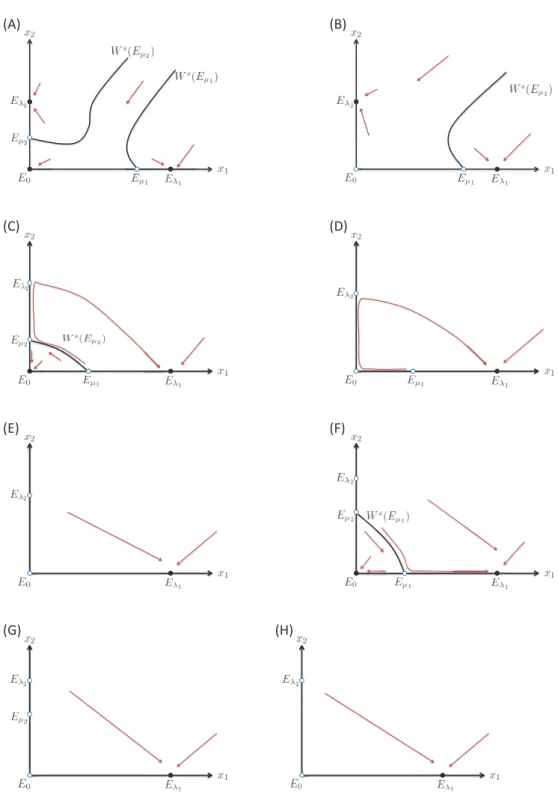
Figure 3: Phase plane (x1, x2, x3) depicts global behavior of 3-species competition. The closed and the open
circles are locally stable and unstable steady states, respectively. Based on the structure of 2-species cases, we can describe the behavior on the boundary planes of Ω. (A) Ws(Eµ1), W
s(Eµ
2) and W s(Eµ
3) separate Ω into four parts, and there is an attractor (E0, Eλ1, Eλ2, Eλ3) in each part. (B) W
s(Eµ
1) and Ws(Eµ2) separate Ω into three parts, there is an attractor (Eλ1, Eλ2, Eλ3) in each part. (C) W
s(Eµ
1) separates Ω into two parts, and there is an attractor (Eλ1, Eλ2) in each part. (D) W
s(Eµ
2) and Ws(Eµ3) separates Ω into three parts, and there is an attractor (E0, Eλ1, Eλ3) in each part. (E) W
s(Eµ
1) separates Ω into two parts, and there is an attractor (Eλ1, Eλ3) in each part. (F) W
s(Eµ
3) separates Ω into two parts, there is an attractor (E, E ) in each part. (G) Eλ is a globally attractor. (H) Ws(Eµ ) separates Ω into two
Chlamydomonas moewusii Chlamydomonas reinhardtiiChlorella pyrenoidosa Chlorella sorokinianaChlorella vulgaris Coelastrum cambricum Coelastrum mircroporum Dictyosphaerium pulchellumMonoraphidium minutum Oocystis sp. Pediastrum boryanumScenedesmus crassus Scenedesmus quadricaudaSelenastrum minutum Chroomonas sp. Cryptomonas cf. ovataCryptomonas erosa Cryptomonas phaseolusCryptomonas sp. Rhodomonas sp. Anabaena cylindrica Anabaena flos-aquae Anabaena macrosporaLimnothrix redekei Phormidium luridum Planktothrix agardhii Synechocystis minima Cosmarium subprotumidumStaurastrum pingue Cymbella tumida Fragilaria bidens Fragilaria crotonensisFragilaria rumpens Fragilaria vaucheriae Gomphonema quadripunctatumGomphonema truncatum Nitzschia gandersheimiensisStephanodiscus neoastraea Ceratium furcoides 10-4 10-3 10-2 10-1 100 101 102 (A)Iin=500;d=0.25 10-4 10-3 10-2 10-1 100 101 102 103 (B)Iin=1000;d=0.25 Chlamydomonas moewusii Chlamydomonas reinhardtiiChlorella pyrenoidosa Chlorella sorokinianaChlorella vulgaris Coelastrum cambricum Coelastrum mircroporum Dictyosphaerium pulchellumMonoraphidium minutum Oocystis sp. Pediastrum boryanumScenedesmus crassus Scenedesmus quadricaudaSelenastrum minutum Chroomonas sp. Cryptomonas cf. ovataCryptomonas erosa Cryptomonas phaseolusCryptomonas sp. Rhodomonas sp. Anabaena cylindrica Anabaena flos-aquae Anabaena macrosporaLimnothrix redekei Phormidium luridum Planktothrix agardhii Synechocystis minima Cosmarium subprotumidumStaurastrum pingue Cymbella tumida Fragilaria bidens Fragilaria crotonensisFragilaria rumpens Fragilaria vaucheriae Gomphonema quadripunctatumGomphonema truncatum Nitzschia gandersheimiensisStephanodiscus neoastraea Ceratium furcoides 10-4 10-3 10-2 10-1 100 101 102 (C)Iin=500;d=0.5 Iout (µmol m-2 s-1) 10-4 10-3 10-2 10-1 100 101 102 103 (D)Iin=1000;d=0.5
Figure 4: Ranges of Ioutwith positive net growth are depicted for 39 species that exibit photoinhibition.
Closed and open circles indicate stable and unstable steady states, respectively. Solid lines indicate intervals where net growth rate is positive. Dotted lines indicate intervals where net growth rate is negative. (A) Low light (Iin= 500) and low loss rate (d = 0.25) condition. (B) High light (Iin= 1000) and low loss rate
0 0.2 0.4 0.6 0.8 1 0 100 200 300 400 500 600 700 800 900 1000
The relative number of species
(A)Monoculture, d=0.25 AL Persistence Extinction 0 0.2 0.4 0.6 0.8 1 0 100 200 300 400 500 600 700 800 900 1000 (B)Monoculture, d=0.5 AL Persistence Extinction 0.001 0.01 0.1 1 0 100 200 300 400 500 600 700 800 900 1000
The relative number of combinations
(C)2-species competition, d=0.25 AL FA 0.001 0.01 0.1 1 0 100 200 300 400 500 600 700 800 900 1000 (D)2-species competition, d=0.5 AL FA ASS+ 0.0001 0.001 0.01 0.1 1 0 100 200 300 400 500 600 700 800 900 1000
The relative number of combinations
Iin (µmol m-2 s-1) (E)3-species competition, d=0.25
AL FA(1) 0.0001 0.001 0.01 0.1 1 0 100 200 300 400 500 600 700 800 900 1000 (F)3-species competition, d=0.5 AL FA(1) FA(2) ASS+(2) ASS+(3)
Figure 5: Results of numerical experiments. Monoculture growth with low (A) and high (B) loss rates; 2-species competition with low (C) and high (D) loss rates; and 3-species competition with low (E) and high (F) loss rates. Other model parameters are: Kbg = 0.2 and zmax = 1. Outcomes are evaluated by
the relative number of species or species combinations for each Iin. AL indicates a strong Allee effect,