寬頻光都會與接取網路之關鍵技術－總計畫:寬頻光都會與接取網路之關鍵技術(2/3)

(1)

行政院國家科學委員會專題研究計畫期中進度報告

寬頻光都會與接取網路之關鍵技術--總計畫:寬頻光都會與

接取網路之關鍵技術(2/3)

期中進度報告(精簡版)

計畫類別：整合型計畫編號： NSC 95-2221-E-002-185- 執行期間： 95 年 08 月 01 日至 96 年 07 月 31 日執行單位：國立臺灣大學電機工程學系暨研究所計畫主持人：吳靜雄公開資訊：期中報告不提供公開查詢

中華民國 96 年 06 月 01 日

(2)

行政院國家科學委員會專題研究計劃成果報告

寬頻光都會與接取網路之關鍵技術─總計劃(2/3)

計劃編號： NSC-95-2221-E-002-185 執行期限：95 年 8 月 1 日至 96 年 7 月 31 日主持人：吳靜雄教授共同主持人：曹恆偉教授李三良教授李揚漢教授曹士林教授執行單位：台大電機系台科大電子系淡江電機系師大光電所

一、

中文摘要

為因應急速增加的頻寬需求，光纖網路已成為建構寬頻資訊網路的主要媒介。為了有效利用光纖的高容量特性，分波多工(WDM)、分碼多工(CDMA) 及分時多工 (TDMA) 為常見的傳輸方式。同時，高速的路由交換與波長轉換元件為發展光纖網路的關鍵技術。本整合型計畫希望能針對高速光通訊系統與元件之設計進行研究。在高速光通訊系統設計方面，本計畫中研究於馬可夫模型之自相關傳輸量輸入下的光封包交換機之效能；同時本計畫研究及二維光分碼系統之特性，並藉由上述之研究將二維光分碼應用於被動光網路以實現寬頻接取服務。在元件設計方面，本計畫研究異質積體化技術以將製作於不同基材的多功能元件整合在同一基板上，以結合光通訊模組所需的光學與電路，降低成本並增加可靠度；另外本計畫也研究價格低廉且體積小的光學共振腔式(etalon)光濾波器元件及二段式分佈反饋雷射展示其單模與多模競爭之全光時脈回復機制。關鍵詞：分波多工，分碼多工，被動光網路，可調波長雷射，波長轉換，光封包交換 Abstract

The optical fiber plays an important role in the broadband wireline communication networks. Three techniques: wavelength division multiplex (WDM), code division multiple access (CDMA) and time division multiple access (TDMA) are most commonly used transmission schemes to efficiently utilize the large bandwidth provided by the fiber. The optical communication devices such as high speed packet switch and wavelength converter are the key components in the optical communication networks. This integrated project studies the high-speed optical communication systems and the design of the optical components.

(3)

In this project, we investigate optical packet switches under Markovian modeled self-similar traffic input. We also investigate a 2D OCDMA system which can be applied to the passive optical network which is a solution to realize the full service access network. For the design of the optical components, in order to combine the optical communication modules with the required optic components and electrical circuit, to reduce the cost, and to increase the reliability, we investigate the hetero-integration technology to fabricate the devices of different substrates in one substrate. In addition, we also investigate the low cost and small area etalon optic filter and demonstrate all-optical clock recovery under the psuedorandom bit sequence data injection by using a two-section DFB laser when it was biased at the self- pulsating condition in single mode or in multi-mode competition case.

二、

重要研究成果

I. 子計畫一網際網路已融入人們日常生活中，也是資訊取得及傳播的利器，因其用戶數迅速增加，寬頻需求殷切，一個好的交換技術是必須要的，而光封包交換技術結合了分波多工的技術，具備了高速交換能力，高資料傳輸速度與格式通透性，在未來即將在通訊領域中扮演重要的角色。本研究主題為(1)於馬可夫模型之自相關傳輸量輸入下的光封包交換機之研究及 (2)二維光分碼系統特性之探討。首先，我們研究使用部分緩衝分享機制下之光封包交換機在馬可夫模型之自相關傳輸量輸入下的封包遺失行為。兩種優先權的分類在此被考慮，此兩者都是自然自相關，且靠著兩個獨立的馬可夫抵達程序來近似。緩衝記憶體的門檻值把佔領緩衝記憶體的狀態空間分成兩個部分，當此週期時間被假設成隨意發生，此種分割將依次給予緊要的與非緊要的週期時間。因此，我們研究與分析短時間與長時間的效能估量，恰當的分析結果已被計算出且被模擬結果所驗證，當光交換機在自相關傳輸量輸入下提供不同的服務時，我們的分析對於最佳化的緩衝記憶體控制是有用的。其次，我們將指出分波多工的光封包交換機若使用波長轉換時，在馬可夫模型之自相關傳輸量輸入下，其效能會因採用波長轉換的技術而有好處。我們已經計算出分析的結果，且被模擬所驗證，我們提出一種程序去計算數值結果，並減少了計算的時間與複雜度，在獲得分波多工之光封包交換機的滿意效能上，我們的分析是非常有用的。最後，我們探討二維光編碼的特性，並研究系統架構，在光域上分波多工不需考慮同步問題，但在時域編碼分為同步及非同步兩種，我們比較各種編碼之後發現完美差異碼具許多優點，所以我們將其應用在系統中並完整的評估其效益，數值結果顯示此系統之同時使用者數目及錯碼率均優於其他系統。另外，因光纖已被大量使用，我們也提出二維光域及空域接取網路。

(4)

詳細內容請參考附件一。 II. 子計畫二本子計畫研究供都會網路及接取網路應用的光電主動元件模組，並研發異質積體化技術以將製作於不同基材的多功能元件整合在同一基板上，以結合光通訊模組所需的光學與電路，降低成本並增加可靠度。我們使用一個價格低廉且體積小的光學共振腔式(etalon)光濾波器元件，放置於 10Gbps 直調雷射的輸出端，可以達到抑制頻率啁啾效應進而延伸傳輸距離的目的，從小於 10 公里增加到大於 75 公里，實驗結果可以對 2 個 10Gbps 直調雷射同時進行補償，因此利用 etalon 的週期性頻譜變化的特性，證實可以同時對多個通道的直調雷射傳輸系統達到性能改善的效果。我們就二段式分佈反饋雷射展示其單模與多模競爭之全光時脈回復機制，且使用光學濾波器可使全光時脈回復機制同時在多模態下進行。詳細內容請參考附件二。 III. 子計畫三 本計劃中，針對同步光分碼多工存取系統架構做討論，為了讓系統模擬更符合實際上現象，考慮了接收端使用者的功率會隨著傳送距離遠近而有大小差異的條件，因此在傳統發射同步型的訊框格式下，當考慮使用者接收之功率不同時，會影響整體的系統效能。針對此問題我們提出了接收同步型的架構，藉由估測出距離相對之時間使每個使用者到達耦合器之時間相同，並將訊框格式加以改善，加強使用者間相互干擾的偵測，提升系統效能。最後，我們利用模擬軟體，建構及模擬六組使用者之同步光分碼多工存取系統在發射同步型和接收同步型架構下的效能比較。詳細內容請參考附件三。 IV. 子計畫四本子計畫研究重點在於光分碼多工（OCDMA）接收機電路製作，以及光通信網路中信號品質監測之研究。為了增加 PON 網路使用者數目及傳輸容量，實際應用多以分時多工機制來達成，然而其仍具有頻寬使用不佳的缺點存在。本計畫根據完美相差碼所建構的分碼多工機制，設計出接收機前端電路並以台積電 0.35 微米 CMOS 製程完成實作。此外，為了進行光信號品質之即時監測，本計畫另一部份利用非同步光域取樣的方式，根據所得之統計資訊來進行光信噪比（OSNR）之估測。本計畫所製作的光分碼多工接收電路，包括轉阻放大器（TIA）、可變增益放大器（VGA）、後級放大器與類比相關器（Analog Correlator），以上元件均整合於同一晶片上。為了有效提高電路頻寬，我們採用共閘形式的轉阻放大器，在可變增益放大器與後級放大器則採用主動回授的設計方式。在相關器方面，利用改良式 Gilbert 電路的架構，能夠對完美相差碼進行相關運算。經過測試，本電路在 1.25GHz 的展頻碼與 3.3 伏特輸入電壓之下，總消耗功率為 452mW 且可正常工作。在信號品質監測之研究方面，非同步光域取樣是本計畫的研究主題。藉由光域非同步取樣所得之統計直方圖

(5)

（Histogram），我們可以統計與曲線擬合的方法得到與光信噪比（OSNR）有關的參數。然而在即時監控的應用上，如何能以較少的取樣數獲取足夠且可靠的資訊仍是值得研究的課題。因此我們對取樣時脈進行三角波頻率調變，經模擬驗證（OptiSystem）後發現在 10Gb/s 不歸零碼傳輸應用中，在取樣數為 8192 點即可得到良好的監測參數性質。同時在 10Gb/s±50ppm 的系統時脈運作下都可得到一致的結果，達成位元速率透明性（bit-rate transparency）的理想。詳細內容請參考附件四。 V. 子計畫五在最近幾年，光子晶體光通訊元件設計上已逐漸廣泛的被研究應用，現行在產業及學術研究上也充分的被應用及開發，然而光通信元件之縮小化亦為必然趨勢，因此，本計畫即是以縮小現有光通信元件，並朝向光學能隙晶格光通信元件的技術進行研發為目的。本計畫為“下世代光子晶體內嵌式光交換器元件設計、製作及應用於寬頻都會與擷取網路平台之研究＂總計畫之一部份，並分三年進行，第一年已完成光學能隙晶格光子晶體光波導光通信元件系統之研究，並建立模擬環境及測量元件基礎環境，並建立微細光纖抽拉裝置結合設計及模擬矽上微腔盤光記憶儲存單位，以輸入光至微腔盤的共振條件成立與否去決定信號光是否在腔盤中儲存其光能量。本年度為計劃第二年，目前已完成利用矽上絕緣層矽晶元件建立光學讀取系統結合多模干涉型光學能隙波導光分歧器及光子晶體Mach-Zehnder 結構，並與第一年之光學能隙晶格光子晶體光波導光通信元件系統整合。進度正常依計劃進行，未來第三年將進行32x32矽上絕緣層矽晶為基底奈米光學光波導及波長可交換式微波光子晶體光控開關主動元件光通信元件之研究及整合，以應用於新世代高速光通信系統之中。本計畫完成研究矽上絕緣層矽晶元件建立光學讀取系統結合多模干涉型光學能隙波導光分歧器及光子晶體 Mach-Zehnder結構。我們利用二維光子晶體週期性結構及線狀缺陷的技術並針對不同的能隙結構來控制光在光子晶體波導中行進的路徑，以便達到縮小積體光學元件之體積。多模干涉型光學能隙波導光分歧器是基於自成像現象設計而成。我們利用自成像現象在矽上絕緣層矽晶脊狀光波導設計多模干涉光分歧器並進一步研究自成像現象在光子晶體傳播情形來設計光學能隙波導光分歧器。此外，我們利用六角形晶格光子晶體的 Mach-Zehnder結構來達成干涉現象，並藉此設計光學信號讀取系統。詳細內容請參考附件五。

三、

計畫成果自評與討論

本計畫在光纖通訊研究上有相當多的成果，包括了高速光通訊系統之效能分析，光分碼多工之編碼研究，光封包交換技術及其效能，異質積體化技術光學共振腔式(etalon)光濾波器元件，已有許多專利及論文發表，成果豐富。

(6)

行政院國家科學委員會專題研究計劃成果報告

高速光子交換及被動接取光網路之研究─子計畫一

(2/3)

計劃編號： NSC-95-2221-E-002-184 執行期限：95 年 8 月 1 日至 96 年 7 月 31 日主持人：吳靜雄教授

參與人員：Malla Reddy Perati、黃富源、邱建林、楊有為、陳仲軒、吳柏毅、

余靖涵、陳培霖、戴嘉瑩

中文摘要

網際網路已融入人們日常生活中，也是資訊取得及傳播的利器，因其用戶數迅速增加，寬頻需求殷切，一個好的交換技術是必須要的，而光封包交換技術結合了分波多工的技術，具備了高速交換能力，高資料傳輸速度與格式通透性，在未來即將在通訊領域中扮演重要的角色。本研究主題為(1)於馬可夫模型之自相關傳輸量輸入下的光封包交換機之研究及 (2)二維光分碼系統特性之探討。首先，我們研究使用部分緩衝分享機制下之光封包交換機在馬可夫模型之自相關傳輸量輸入下的封包遺失行為。兩種優先權的分類在此被考慮，此兩者都是自然自相關，且靠著兩個獨立的馬可夫抵達程序來近似。緩衝記憶體的門檻值把佔領緩衝記憶體的狀態空間分成兩個部分，當此週期時間被假設成隨意發生，此種分割將依次給予緊要的與非緊要的週期時間。因此，我們研究與分析短時間與長時間的效能估量，恰當的分析結果已被計算出且被模擬結果所驗證，當光交換機在自相關傳輸量輸入下提供不同的服務時，我們的分析對於最佳化的緩衝記憶體控制是有用的。其次，我們將指出分波多工的光封包交換機若使用波長轉換時，在馬可夫模型之自相關傳輸量輸入下，其效能會因採用波長轉換的技術而有好處。我們已經計算出分析的結果，且被模擬所驗證，我們提出一種程序去計算數值結果，並減少了計算的時間與複雜度，在獲得分波多工之光封包交換機的滿意效能上，我們的分析是非常有用的。最後，我們探討二維光編碼的特性，並研究系統架構，在光域上分波多工不需考慮同步問題，但在時域編碼分為同步及非同步兩種，我們比較各種編碼之後發現完美差異碼具許多優點，所以我們將其應用在系統中並完整的評估其效益，數值結果顯示此系統之同時使用者數目及錯碼率均優於其他系統。另外，因光纖已被大量使用，我們也提出二維光域及空域接取網路。附件一

(7)

Abstract

Internet has been utilized worldwide, the number of users grow rapidly. The demand of bandwidth increases tremendously. A good switching technology is required, and optical packet switching (OPS) incorporating with wavelength division multiplexing (WDM) technology, which has high-speed switching capability, high data rate and format transparency, is an attractive in the near future. The topics of this search are to investigate optical packet switches under Markovian modeled self-similar traffic input and optical code division multiple access (OCDMA) system.

First, we investigate the loss behavior of optical packet switches (OPSes) employing partial buffer sharing (PBS) mechanism to provide differentiated services under Markovian modeled self-similar traffic input. Two priority classes are considered; both are self-similar in nature and are fitted by two independent Markovian arrival processes (MAPs). The level of buffer threshold divides the state space of the buffer occupancy into two parts. Such a partition in turn gives the critical and non-critical periods which are assumed to occur alternatively. Accordingly, we investigate and analyze both the short term and long term performance measures. Pertinent analytical results are computed and then verified by simulation. Our analysis is useful in telling the optimal control of buffer of

OPS handling self-similar traffic to provide differentiated services.

Second, we make the switching performance of wavelength division multiplexing (WDM) optical packet switch (OPS) employing wavelength conversion (WC) techniques under Markovian modeled self-similar traffic input to point the benefit of wavelength conversion. The analytical results are calculated and verified by simulation. We propose a procedure to calculate the numerical results in order to reduce the effort of computation. The computation complexity of the analysis is then presented. Our analysis is useful in dimensioning the WDM OPS to obtain satisfactory performance.

Last, we study two-dimensioned (2-D) Optical Code Division Multiple Access (OCDMA) techniques, several 2-D OCDMA systems were investigated, we have found that the Perfect Difference Code (PDC) have many advantages. Therefore the spectral/time OCDMA system utilizing PDC is investigated completely. The results show that this system has good performance. In

addition, because the fibers are deployed in the cities and many residential areas, we also propose a spectral/spatial 2D OCDMA system, which may also applicable for wideband access network.

Keywords: Differentiated service, Markovian arrival process, matrix-analytic method, partial buffer sharing, self-similar traffic, MAM, MAP,

(8)

self-similar traffic, WDM optical packet switch, wavelength conversion, OCDMA, perfect difference code.

一、

研究內容與討論

(1) Loss Behavior Analysis of Optical Packet Switches Employing Partial Buffer Sharing Mechanism under Markovian Modeled Self-Similar Traffic Input

I. Queiueing Model of OPS Employing PBS Mechanism

Currently, due to the lack of optical random access memory (ORAM), only the passive type buffer management schemes are feasible to be realized in the high-speed optical switching nodes. Among the passive buffer management schemes, PBS mechanism is the most suitable one for OPS. This is because (1) optical buffers consisting of FDLs with fixed delay granularity can not arbitrarily hold the packets for a random amount of time, (2) the erasable optical buffers are not available yet for implementing push-out scheme. Also, due to the implementation, OPS of output queueing type is most feasible. Hence, the equivalent queueing model of a specific output port of the OPS with a service discipline of first-come-first-serve (FCFS) is equal to that of a multiplexer.

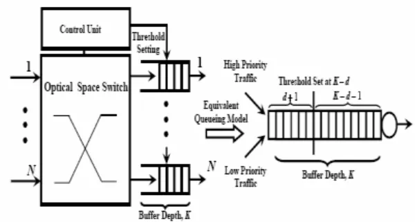
A general block diagram of OPS employing PBS mechanism is shown in the left hand side of Fig. 1, where there

are N input ports and N output ports each having K +1 fiber delay lines (FDLs) constituting the optical buffers with buffer depth K. When the input traffic is with a fixed packet length and the OPS is operating at a synchronous mode, then the suitable choice of the delay unit, h, in each FDL is to let h equal the packet length of the input traffic measured in time. Consequently, the equivalent queueing model of one specific output port of the OPS employing PBS mechanism can be depicted in the right hand side of Fig. 1, in which, a buffer with buffer depth K and a threshold set at the buffer level

, 0

K−d d≥ [21]. As shown in Fig. 1,

the low priority packets can only access the ‘K− −d 1’ buffer spaces, whereas the high priority packets can utilize the whole buffer space regardless of the threshold levelK−d. Accordingly, we can define the “critical period” as the time period during which the buffer occupancy is greater than or equal to

K−d, and the “non-critical period” as the time interval during which the buffer occupancy is less than K−d [19], [21]. In this report, we assume that the packet length is fixed and constant. Hence the resultant queueing system of OPS employing PBS mechanism handling Markovian modeled self-similar traffic with fixed packet length is equivalent to an MAP/D/1/K queue with PBS policy.

(9)

Fig. 1 A general block diagram of the OPS employing PBS mechanism and the equivalent queueing model of a specific output port of the same one with two different priority traffic input.

II Loss Behavior Analysis

Now we could analyze the loss behavior of OPS employing PBS mechanism with MAP modeled self-similar input traffic. For the sake of simplicity, two priorities are considered. Each priority traffic is characterized by a MAP emulating self-similar process. Higher priority (class 1) and lower priority (class 2) packets arrive at the system according to MAPs of states m₁

and m , respectively. The above MAPs ₂

are characterized by the matrices { (1),C D(1)} and { (2),C D(2)} , respectively. The service time is generally and identically distributed with distribution function H(t). Let

( )

( )( 0, 1, 2) k

m

D t m≥ k= denote the matrices whose ( , )i j th element is the

probability that given departure of class

k at time 0, there is at least one packet

left in the system and the process is in state i, the next departure of class k occurs no later than time t with the

arrival process in state j, and during that service time there are m arrivals. Then

( ) ( ) k m

D t satisfies the following equation

( ) [ ( ) ( ) ] 0 0 ( ) ( ), 1, 2. t k m C k D k z m m D t z e dH k τ _τ ∞ + = = =

∑

∫

When service time is deterministic and is h units/packet, then we have

( ) [ ( ) ( ) ] 0 ( ) ( ), 1, 2. k m C k D k z h m m D t z e u t h k ∞ + = = − =

∑

where u(t) is the unit step function. Therefore, we obtain ( ) [ ( ) ( ) ] 0 ( ) , 1, 2. k m C k D k z h m m D h z e k ∞ + = = =

∑

It is obvious that the matrices D_m( )k can be evaluated by comparing the coefficient of zm on both sides of the above equation. This procedure is outlined in [18], wherein the complete proof or reference is not given. We shall prove the procedure in a simple way and propose a method to tell when the procedure could be terminated. We drop the index k for both classes. Then can be written as [ ] 0 ( ) m C Dz h m m D h z e ∞ + = =

∑

As e[C Dz h+ ] is analytic, we utilize the decay proposition (Cauchy’s estimate) of complex variables as follows.

Proposition 1: Cauchy’s Estimate

Let the matrix function

0

( ) _m m

m

(10)

| |z < . Then for any R ρ such that 0 < ρ < R, one has |a_n|≤M( )ρ ρ−n,n=0,1, 2,3,…, where | | ( ) max | ( ) | z M a z ρ ρ =

= . More precisely, for

a given ε > 0 (in our context, ε is the machine precision of the floating point arithmetic) ∃N such that

1| i| i N a ∞

= +

∑

has elements at most ε . In view of the Proposition 1 and Taylor

series, [ ] 0 ( ) m C Dz h m m D h z e ∞ + = =

∑

can be rewritten as 0 0 1 ( ) ( ) ( ) ! N m r m m r D h z R z A Bz r ε ∞ = = + = +

∑

where A = Ch, B = Dh and has coefficients with small moduli at most

ε . Hereafter, we drop the argument h in rest of the report for the sake of easiness.

From [ ] 0 ( ) m C Dz h m m D h z e ∞ + = =

∑

, for m=0, we have 0 1 ! r Ar D I r ∞ = = +

∑

where I is the unit matrix of appropriate dimension. For m n. ≥1, let T(n;m) be

the coefficient of zm−1 in (A+Bz)n , the nth term of the series on the right

hand side of [ ] 0 ( ) m C Dz h m m D h z e ∞ + = =

∑

, then we have (1,1) , (1, 2) , ( ,1) n T = A T =B T n =A ( , ) 0, 1, T n m = if m> +n and 2 1 ( ,1) ( , 2) ( , 3) ( , ) ( , 1) ( ) m n n T n T n z T n z T n m z T n n z A Bz − + + + + + + + = + … …

Multiplying both sides by (A + Bz), we obtain 2 1 1 [ ( ,1) ( , 2) ( , 3) ( , ) ( , 1) ]( ) [ ] m n n T n T n z T n z T n m z T n n z A Bz A Bz − + + + + + + + + + = + … …

which could be re-written as

2 1 1 [ ( ,1) ( , 2) ( , 3) ( , ) ( , 1) ]( ) ( 1,1) ( 1, 2) ( 1, 2) . m n n T n T n z T n z T n m z T n n z A Bz T n T n T n n z − + + + + + + + + + = + + + + + + + … … …

Equating the coefficients of like powers of z, we obtain ( 1,1) ( ,1) , T n+ = T n A ( 1, 2) ( , 2) ( ,1) , T n+ = T n A T n+ B ( 1, ) ( , ) ( , 1) , T n q T n q A T n q B q + = + − ∈ Ν

For any positive integer m, D = _m

coefficient of m z in ( ) ! m A Bz m + + coefficient of zm in 1 ( ) ( 1)! m A Bz m + + + + coefficient of z in m 2 ( ) ( 2)! m A Bz m + + + + … ,i.e., ( , 1) ! m T m m D m + = ( 1, 1) ( 2, 1) ( 1)! ( 2)! T m m T m m m m + + + + + + + + + … . Consequently, we obtain ( , 1) , 1, 2, , ! m k m T k m D for m N k ∞ = + =

∑

= …

We then could compute the matrices m

D s for both high priority and low

priority packets. Though the above equation involves infinite number of

(11)

terms, due to the presence of k! in the denominator, only finite number of terms are required to compute the matrices D s . The procedure of _m

computing the matrices D s can be _m

terminated using Proposition 1. The procedure of computing the matrices

m

D s can be terminated using Proposition 1. This is an alternative method to the method proposed in [10], [12], which works well too.

Now consider the embedded Markov chain {L J_n, _n|n≥0} at the departure epochs of the queueing system

on the state space {( , , ) | 0 ,

S = b i j ≤ ≤b K 1≤ ≤i m₁,

2

1≤ ≤j m }, where Ln denotes the buffer

occupancy and Jn denotes the phase of

superposed MAP. For the sake of convenience, a queueing system is said to be at level b, if its buffer occupancy is equal to b−1 (excluding the one at service). Under the operation of PBS mechanism with the level of threshold

, 0

K−d d ≥ , the embedded Markov

chain has an irreducible transition probability matrix P that is given by

( 1 ) ( 1 ) 0 1 1 1 2 1 2 ( 1 ) ( 1 ) 0 1 1 1 2 1 2 ( 1 ) ( 1 ) 0 2 1 2 2 2 ( 1 ) ( 1 ) 3 2 1 2 3 2 ( ) ( ) ( ) ( ) 0 ( 1) 0 0 ( 2) 0 Kd Kd Kd K Kd Kd Kd K Kd Kd Kd K Kd Kd Kd K GD GD GD GC G D D G D D GE K D D D C D D D D E K D D C D D D D E K D C D D D D E K −− − −+ − − − −− − −+ − − − −− −− − − − − −− −− −− − − − ⊗ ⊗ ⊗ ⊗ ⊗ ⊗ − ⊗ ⊗ − … … … … … … … … ( 1 ) ( 1 ) 1 2 3 2 1 2 ( 1 ) ( 1 ) 0 1 2 2 2 ( 1 ) ( 1 ) ( 1 ) 0 2 1 2 1 2 ( 1 ) 0 2 , 0 ( 2) 0 0 ( 1) 0 0 0 ( ) 0 0 0 0 0 (1) d d d D C D D D D E d D C D D D D E d D D D D D D E d E D D − + − − − − − − − − ⊗ ⊗ + ⊗ ⊗ + ⊗ ⊗ ⊗ ⊗ ⎡ ⎤ ⎢ ⎥ ⎢ ⎥ ⎢ ⎥ ⎢ ⎥ ⎢ ⎥ ⎢ ⎥ ⎢ ⎥ ⎢ ⎥ ⎢ ⎥ ⎢ ⎥ ⎢ ⎥ ⎢ ⎥ ⎢ ⎥ ⎢ ⎥ ⎣ ⎦ … … … … … … … … where (1) (2) ' ' ' 0 (2) 2 0 (1) ( ) 2 ' 0 ( ) 1 2 1 ( ), , ( ), ( ) , 1, 2, 3, , , ( ) , C C(1) (2), (1) (2), i i i i i i i i l _{l i} l _i i p D D D D D C D D E p D D p K G C D C D D D − = ∞ − ₌ − − = − − − ⎧ ₌ _⊗ ⎪ ⎪ ₌ ⎪ ⎪ ₌ _⊗ ⎪ ⎪ ₌ _⊗ ₌ ⎨ ⎪ _{= −} ⎪ ⎪ = ⊗ ⎪ = ⊗ ⎪ ⎪⎩

∑

…

In above, the matrix G consists of the conditional probabilities that system is idle. The fundamental arrival rate of

class k packets

is λ( )k =π( ) ( ) , 1, 2,k D k e k= where

( )k

π is the steady probability vector of

C(k)+D(k). Then the traffic intensity is

given asρ =(λ(1)+λ(2)) [E H t( )].

From the operation of PBS mechanism, it is clear that high priority packet loss occurs buffer is full, whereas low priority packet loss happens due to the buffer occupancy threshold. Then, by definition, the steady state high priority packet loss probability (Php) and the steady state low priority packet loss probability (Plp) are respectively given as

hp

P Mean of high priority packet loss

Mean of high priority packet arrival

=

lp

P Mean of low priority packet loss

Mean of low priority packet arrival

=

Firstly, the mean number of high priority and low priority packet arrivals are

(1)

[ ( )]

E H t

λ and λ(2)E H t[ ( )] ,

respectively. Secondly, let 0 1 ( , , , _K) y= y y … y , where 1 2 ,1,1 ,1,2 , , ( , , , ) k k k k m m y = y y … y , ∀k, is the

(12)

probability that departing packet leaves

k packets in the system, i.e., yP = y, ye =

1. And then following [19], the mean of high priority packet loss and the mean of low priority packets loss are respectively given as follows: (1) 0 2 1 (1) 1 2 1 1 ( ) ( ) , K i i K k K k i k i iy G D D e iy D D e ∞ + − = ∞ − + + − = = ⊗ + ⊗

∑

∑ ∑

2 (1) (2) ( 1) 0 1 1 0 1 (1) (2) ( 2) (2) 1 1 1 1 0 (2) 1 ! 1 [ ] [ ] [ ] K d K d j K d j i i j K d K d k K d k k j K d k j i i k i j K k i k K d i D iy G D D D e iy D D D D e iy D D e − ∞ − _{− +} − − + − = = − ∞ − − + − + + − − + − + − = = = ∞ − = − + = ⊗ ⊗ + + ⊗ + ⊗ + ⊗ ∑ ∑ ∑ ∑ ∑ ∑ ∑ where ₁ (1) 0 i i D₋ =

∑

∞₌ D . Thus we can calculate the steady state high priority packet loss probability, P , and the hp

steady state low priority packet loss probability, P .lp

Next, we proceed to calculate the mean lengths of critical and non-critical periods which are assumed to occur alternatively. Since the non-critical period is defined as the time period over which the number of packets in buffer (with buffer depth, K) is less than the threshold K−d, and the critical period is defined as the time period over which the number of packets in buffer is greater than or equal to the threshold

K−d, we could decompose the state space S into two subsets:

1 2 1 2 {( , , ) | 0 1,1 ,1 }, {( , , ) | ,1 ,1 }. nc c S b i j b K d i m j m S b i j K d b K i m j m = ≤ ≤ − − ≤ ≤ ≤ ≤ = − ≤ ≤ ≤ ≤ ≤ ≤

This partition of S makes the matrix P decomposed as follows: , , nc nc c c nc c P P P P P ⎡ ⎤ = ⎢ ⎥ ⎣ ⎦ where 0 1 2 1 0 1 2 1 0 3 2 4 3 0 1 0 0 0 0 0 K d K d K d K d K d K d nc K d K d GD GD GD GD D D D D D D D P D D D D − − − − − − − − − − − − − − − − ⎡ ⎤ ⎢ ⎥ ⎢ ⎥ ⎢ ⎥ = ⎢ ⎥ ⎢ ⎥ ⎢ ⎥ ⎢ ⎥ ⎢ ⎥ ⎣ ⎦ … … … … … , (1) (1) 1 2 1 2 (1) (1) 1 2 1 2 (1) (1) 1 2 2 2 , (1) (1) 2 1 2 3 2 (1) (1) 2 3 2 1 2 ( ) ( ) ( ) ( ) ( 1) ( 2) ( 2) K d K d K K d K d K K d K d K nc c K d K d K d GC G D D G D D GE K C D D D D E K C D D D D E K P C D D D D E K C D D D D E d − − + − − − − − + − − − − − − − − − − − − − − − − − + − ⎡ ⊗ ⊗ ⎤ ⎢ _⊗ _⊗ ⎥ ⎢ ⎥ ⎢ _⊗ _⊗ ₋ = ⎢ ⊗ ⊗ − ⎢ ⎢ ⎢ ⎢ ⊗ ⊗ + ⎣ ⎦ … … … … … ⎥ ⎥ ⎥ ⎥ ⎥ ⎥ , 0 , 0 0 0 0 0 0 0 , and 0 0 0 0 c nc D P ⎡ ⎤ ⎢ ⎥ ⎢ ⎥ = ⎢ ⎥ ⎢ ⎥ ⎣ ⎦ … … … (1) (1) 1 2 2 2 (1) (1) (1) 0 2 1 2 1 2 (1) 0 2 ( 1) ( ) 0 0 (1) d d c C D D D D E d D D D D D D E d P D D E − − − − − − − ⎡ ⊗ ⊗ + ⎤ ⎢ _⊗ _⊗ _⊗ ⎥ ⎢ ⎥ = ⎢ ⎥ ⎢ ⎥ ⊗ ⎢ ⎥ ⎣ ⎦ … … …

The sub-matrices Pnc, Pnc;c, Pc;nc, and Pc

are the left upper part, right upper part, left lower part, and right lower part of the matrix P, that correspond to the transitions of those from Snc into itself,

from Snc into Sc, from Sc into Snc, and

from Sc into itself, respectively.

For the case of non-critical period, consider the transition probability matrix of absorbing Markov chain with transient states Snc and absorbing states

Sc, , , 0 nc nc c nc P P P I ⎡ ⎤ = ⎢ ⎥ ⎣ ⎦

where I and 0 are the unit matrix and zero matrix of appropriate dimensions. If Y is the random variable standing for the number of steps taken prior to

(13)

absorption, then the kth factorial moment of Y following from the probabilistic arguments is as follows [22], 1 [ ( 1) ( 1)] ! _nck ( _nc) k E Y Y Y k k βP − I P − e = − − + = − …

where β is the initial probability

vector of transient states and is of the form [0, 0,…, 0,β_{K d}_{− −}₁]. This is followed from the fact that buffer occupancy starts at K− −d 1 in every non-critical period except the first one. The vector ¹0 is the zero vector of appropriate dimension. Similarly, for the case of critical period, consider the transition probability matrix of absorbing Markov chain that has transient states Sc and absorbing states

Snc, , 0 c nc c c I P P P ⎡ ⎤ = ⎢ ⎥ ⎣ ⎦

If Z is the random variable standing for the number of steps taken prior to absorption, then the kth factorial moment of Z is given by [22] 1 [ ( 1) ( 1)] ! _ck ( _c) k , E Z Z Z k k αP − I P − e = − − + = − …

where α is the initial probability vector of the transient states. Now the problem of finding the mean lengths of critical and non-critical periods are reduced to the problem of finding the initial probability vectors α and β , which can be computed as follows.

Consider the first absorbing Markov chain. Let rij be the probability

of being absorbed in the state ,i j∈ , S_c

starting in transient state ,i j∈S_nc . Then for each j∈S_c , we have the following relation nc ij ij is sj s S r q q r ∈ = +

∑

In the above relation, the first term corresponds to a transition from transient state to absorbing state directly, whereas the second term corresponds to the transitions from a transient state to other transient states and then to absorbing state. The above relation can be written in matrix form as follows:

, , nc nc c nc nc R =P +P R 1 , . ., _nc ( _nc) _{nc c}. i e R = −I P − P

The matrix (I−P_nc)−1 is the fundamental matrix of the absorbing Markov chain under consideration. Rnc is

the transition matrix where the chain starts in transient states and ends up in an absorbing state. Similarly for the case of the second absorbing Markov chain, analogous to Rnc, we have the matrix Rc

that can be obtained as 1

,

( ) ' ,

c c nc c

R = −I P − P

where P'_{nc c}_, is the last column of the matrix Pc;nc and is equal to [D₀, 0,…, 0].

The matrix P'_{nc c}_, is followed from the fact that for a non-critical period, it

(14)

suffices to attain the buffer K− −d 1 level rather than all other below levels, the level of buffer occupancy K− −d 1 is the starting point of non-critical period of each cycle except the first one. The matrix (I−P_c)−1 is the fundamental matrix of the second absorbing Markov chain. Since the critical and non-critical periods are assumed to occur alternatively, the initial distribution vector of transient states of one of the two aforementioned absorbing Markov chains would be the absorbing probability vector

of the other. Hence, we have

1 and .

K d Rc Rnc

β _{− −} =α α β=

Taking the definition of β into

account, the above equation can be written as

1 and 1 ' ,

K d Rc K d R nc

β _{− −} =α α β= _{− −}

where 'R _nc is the product of the last

m1m2 rows of R_c = −(I P_nc)−1 and Pnc;c.

The two vectors β_{K d}_{− −}₁ and α can be

computed by solving

1 and 1 ' ,

K d Rc K d R nc

β _{− −} =α α β= _{− −}

iteratively, on assigning arbitrary values to either β_{K d}_{− −}₁ or α first. Following the above discussions and the matrix analytic methods [12], [19], [22], [23], we could compute the following

performance measures:

1) Steady state packet loss probabilities, 2) Mean lengths of critical and non-critical periods.

These two performance measures characterize the long-time and the short-term loss behavior, respectively.

III Approximate Model for Low Priority Traffic

In this report, we further propose an approximate model for the performance analysis of OPS employing PBS mechanism under Markovian modeled self-similar traffic input. Our proposed model is to retain the same high dimensional MAP for high priority traffic, but to reduce the dimension of the resultant MAP of low priority traffic. Obviously, as the number of states of the resultant MAP of low priority traffic decreases, the computation complexity decreases cubically. However, we could not straightforwardly reduce the number of superposed MAPs in fitting the self-similarity for low priority traffic, since this will severely reduce the accuracy of the queueing based performance measures of the resultant MAP.

We have considered three self-similar traffic pertaining to H = 0.7,

H = 0.8, and H = 0.9, all with the mean

arrival rate, λ = 1, variance, σ2 = 0.6, over the time-scale range [10 ,10 ] .. 2 7 For each case, we have a 16-state MAP obtained by using the fitting method discussed in [9]. For all the cases,

(15)

correlation decay rate, ρ , squared coefficient of variation, c , the first 2

three moments, m1, m2, and m3, have been calculated. The correlation decay rate ρ is positive in each case, hence

one could achieve the desired 2-state MAP with these high dimensional MAPs [24]. Moreover, all the cases satisfy the inequalities c2 > 1 and

2 3 1 3 3 ( 1) 2 m c

m > + which are the necessary

conditions to be satisfied by the original distribution in order to have phase-type distribution by matching the first three moments [25]. Following [25], we could have phase type distribution, thereby the approximated 2-state MAP could be obtained.

Table I lists the values of aforementioned traffic descriptors of the original 16-state MAPs, for which we follow the algorithms in [9] to fit a self-similar traffic with mean arrival rate,

λ = 1, variance, σ2

= 0.6, over the time-scale range [102_{; 10}7_{] in three}

different traffic cases with Hurst parameters, H = 0.7, H = 0.8, and H = 0.9, and the corresponding ones of the approximated 2-state MAPs.

Table I: Statistics of Original MAPs and Approximated 2-State MAPs.

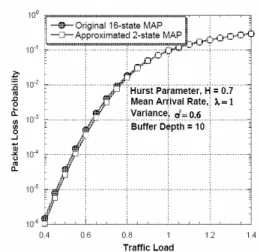
We illustrate the packet loss probability against the traffic load for the MAP/D/1/K queues under the inputs of the above two MAPs with traffic descriptors shown in Table I, when buffer depth equals 10 and H = 0.7 in Fig. 2. From Fig. 2, we observe how accurate the approximated 2-state MAP is. The figures in the cases of H = 0.8 and H = 0.9 could not be shown here. However, we do observe that the accuracy of the approximation becomes worse when H increases. By applying this approximate model, it is obvious that the computation complexity is reduced by 83 = 512 times.

(16)

Fig. 2. Packet loss probability against traffic load for the MAP/D/1/K queues under the inputs of the two MAPs with traffic descriptors as shown in Table I, at buffer depth equals 10 and H = 0.7.

IV Simulation Results

We first validate the approximate model by illustrating the comparisons of long term steady state packet loss probabilities against the variable of threshold level, d, at traffic load, L = 0.85, and buffer depth, K = 15, between the analytical results of the approximate model and the simulation results without approximation in Fig. 3. The parameters of the high priority and low priority MAP traffic are the same ones as we shown in Table I.

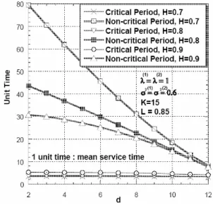
Fig. 4 depicts the mean lengths of the critical and non-critical periods against the threshold level variable, d, for H = 0.7, 0.8, and 0.9. Fig. 5 illustrates the mean lengths of the critical and non-critical periods against the threshold variable, d, when H = 0.8, over 2 different buffer depths. Fig. 6 depicts the mean lengths of the critical

and non-critical periods against the traffic load, when K = 15, d = 9, and H = 0.8. In these figures, the unit time means one unit of the average service time.

From these results, we observe that (1) as d increases, the mean length of non-critical period decreases while the average length of critical period seems to increase slowly (this observation is consistent with the results found in [19], [27], [28]); (2) both the mean lengths of critical and non-critical periods increase, as the buffer depth increases; (3) the mean length of non-critical period decreases drastically as traffic load increases whereas the mean length of critical period increases moderately as traffic load increases; (4) the higher the Hurst parameter is, the lower the mean length of non-critical period is; while the mean length of critical period increases as Hurst parameter increases.

From the information of the mean lengths of critical and non-critical periods, it is very likely that we could adopt these measures as a trigger event of initializing call admission control scheme in OPS to improve the switching performance to greater extent.

(17)

Fig.3 The steady state packet loss probabilities against the variable of threshold level, d, at traffic load L = 0.85 at various H.

Fig. 4 The mean lengths of critical and non-critical periods against the threshold variable, d, at buffer depth K = 15, traffic load L = 0.85, and over three different Hurst parameters.

Fig. 5 The mean lengths of critical and non-critical periods against the threshold variable, d, at L = 0.85, H = 0.8, and over two different buffer depths.

Fig. 6 The mean lengths of critical and non-critical periods against the threshold variable, d, at K = 15, d = 9, and H = 0.8.

(18)

(2) WDM Optical Packet Switches Employing Wavelength Conversion in Conjunction with Markovian Modeled Self-Similar Traffic Input

I Queueing Model and Related Formulae

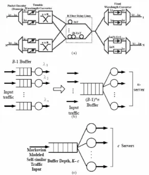
The architecture of WDM OPS employing wavelength conversion techniques implemented in a broadcast-and-select architecture is shown in Fig. 7(a), in which, there are N input ports and N output ports, and each port has n wavelength channels,

1, 2, , n

λ λ … λ in it. B FDLs constitute the optical buffers with buffer depth (B− ). 1 For the sake of simplicity, we assume that the packet length is fixed and constant, and that the packet length is equal to h units when it is measured in time. Further, we assume that the WDM OPS is operating at a synchronous mode with delay time unit, T, for the FDLs of optical buffers, where the suitable value of delay time unit, T, is chosen to be h, the packet length measured in time. No specific scheduling algorithm is applied, only the service discipline of first-come-first-serve (FCFS) is adopted. Hence, the queueing model of a specific output port of such OPS is equivalent to the one of a multiplexer. When the wavelength conversion is employed, the equivalent queueing model is shown in Fig. 7(b). When the traffic aggregated at the input end of the optical buffers of one of the specific output ports is MAP modeled self-similar processes, then, the

final queueing model is a MAP/D/c/K queueing system as shown in Fig. 7(c). As illustrated in Fig. 7(c), the number of wavelength channels per port, n, is equal to the number of servers, c, and the total effective buffer size of optical buffers, (B− )n as shown in Fig. 7(b), is equal 1 to the buffer depth of the MAP/D/c/K queue, K−c. Therefore, the problem of analyzing WDM OPS employing wavelength conversion techniques is equivalent to solving the MAP/D/c/K queueing systems with the parameters mentioned above.

Fig. 7 (a) A block diagram of WDM OPS implemented in broadcast-and-select architecture; (b) the equivalent queueing model of a specific output port of WDM OPS employing wavelength conversion; (c) the final equivalent

MAP/D/c/K queue.

Let H(t) be the generally and identically distributed service time. Let

( ), 0 n

(19)

whose ( , )i j th element represents the

conditional probability that n customers arrive at the system during service time and the underlying Markov chain is in phase j at the end of service given that the underlying Markov chain is in phase

i at the beginning of the service. Then

( ) n

A t satisfies the following equation

[ ] 0 0 ( ) n t C Dz ( ). n n A t z e τdH τ ∞ + = =

∑

_∫

When the service time is deterministic and is h units/packet, then the above formula is reduced to [ ] 0 0 1 ( ) [ ] , ! n C Dz h r n n r A t z e A Bz r ∞ ∞ + = = = = +

∑

where A = Ch, B = Dh.

It is obvious that the matrices A s _n

of counting function can be obtained by comparing the coefficients of z on n

both sides of the above equation. A procedure to calculate the matrices of counting functions [19] is briefed as follows. Hereafter, for the sake of easiness, we drop the argument h in rest of the report. For n = 0, the above formula will be 0 1 , ! r r A A I r ∞ = = +

∑

where I is the unit matrix of appropriate dimension. And the rest of A s can be _n

obtained as follows. ( , 1) , 1, 2, , ! n k n T k n A for n N k ∞ = + =

∑

= …

where ( , )T i j can be calculated using

the recurrence formulae as follows ( 1, ) ( , ) ( , 1) ,

T i+ j =T i j A T i j+ − B j∈ N

Though A involves infinite number of _n

terms, due to the presence of k! in the

denominator, only finite number of terms are required to compute the matrices A s . The procedure of _n

computing the matrices A s can be _n

terminated using Cauchy estimate as shown in the Proposition 1 to avoid lots of computation efforts.

Next, we consider the embedded Markov chain { ( ), ( )}, L n J n n≥ , at 0 the departures of the queueing system on

the state space {0,1, 2,…,K− ×c} {1, 2,…, }m , where

L(n) and J(n) denote the buffer

occupancy and the state of MAP, respectively. At the steady state, the transition probability matrix corresponding to the departure points, P

(with the dimension (K− +c 1)m×(K− +c 1)m ), is as follows: 0 1 2 1 0 1 2 1 0 1 2 1 0 1 2 1 0 2 1 2 1 0 1 . 0 0 0 K c K c K c K c K c K c K c K c K c K c K c K c K c K c K c c c A A A A B A A A A B A A A A B P A A A A B A A A B A A B − − − − − − − − − − − − − − − − − − − − − − − ⎡ ⎤ ⎢ ⎥ ⎢ ⎥ ⎢ ⎥ ⎢ ⎥ ⎢ ⎥ = ⎢ ⎥ ⎢ ⎥ ⎢ ⎥ ⎢ ⎥ ⎢ ⎥ ⎢ ⎥ ⎣ ⎦ … … … … … … … … … … … …

In the matrix, P, elements of the first (c + 1) rows are identical and

n _{i n} i

B =

∑

∞₌ A denote the probability that there are at least n arrivals. A s are _n

computed following the algorithm in the aforementioned procedure. Next, let x_k, 0≤ ≤ −k K c , denote a 1 m× vector whose ith element represents the

(20)

steady state probability that the number of packets in the system at departures is

k and the phase of the arrival process is i.

At the steady state, we could find the vector { }x= x , according to the steady _k state equations xP = x, xe = 1.

Although the general relationship between the probability generating function of queue length at arbitrary time points and at departure points holds good [33] in the case of multiple server queues with finite buffer, the nature of multi-server makes it hard to establish an explicit formula for packet loss probability unlike the single server case in conventional researches [8]. Instead, we compute the loss probability using the steady state probability vector at departure epochs owing to fact that packet loss is due to buffer overflow.

Let PL denote the number of packets lost due to the fact that buffer is full. Then the expected value of PL is given as 0 1 [ ] K c i K i j i j E PL j A − ∞ − + = = =

∑∑

x e

by considering the last column of the (K− + ×c 1) (K− + block transition c 1) probability matrix P. Then the packet loss probability, PLP, can be obtained by [ ] [ ( )] E PL PLP E H t λ =

where ¸ λ E[H(t)] is the number of packet arrivals during the mean service time.

II Steady state Probability Vector

From the above subsection it is

clear that problem of finding packet loss probability is reduced to the problem of finding steady state vector. It is worthwhile and interesting to investigate the required computation complexity of calculating the steady state probability vector. To the best of our knowledge, this analysis of the computation complexity pertaining to the MAP/D/c/K queueing systems is not available yet and is useful in deciding the necessary platform for analyzing WDM OPS employing wavelength conversion under Markovian modeled self-similar traffic input.

First, we shall present a method to compute the steady state probability vector, and then we derive the computation complexity of the same as follows. The matrix P is not of the canonical M/G/1 type. However, it is possible to exploit Schur-Banachiewicz inversion formula to P, which has been used to compute the steady state probability vector when P is in canonical form [12]. Accordingly, the steady state probability vector x is given by x = [0, 0,…, 0,1](I−P₁)−1, where I is the unit matrix of appropriate dimension

and P is the matrix P in which the last ₁

column is replaced by [ 1, 1,− − …, 1, 0]− T. Let [E_{K c}₋ ,E_{K c}₋ ,…,E_{K c}₋ ,E_{K c}_{− −}₁,…,E_c]T be the last column of P . Multiplying ₁

the permutation matrix S by (I−P₁), we have

(21)

1 0 1 2 1 0 2 1 2 1 0 1 0 1 2 1 0 1 2 1 0 1 2 1 ( ) 0 0 0 , K c K c K c K c K c K c c c K c K c K c K c K c K c K c K c K c S I P A A A A E A A A E A A I E I A A A A E A I A A A E A A I A A E − − − − − + − − − − − − − − − − − − − − − − − − = − − − − − ⎡ ⎤ ⎢ ₋ ₋ ₋ ⎥ ⎢ ⎥ ⎢ ⎥ ⎢ ₋ ₋ ₋ ⎥ ⎢ ⎥ ⎢ − − − − ⎥ ⎢ ⎥ − − − − − ⎢ ⎥ ⎢ ⎥ ⎢ ⎥ − − − − ⎢ ⎥ ⎣ ⎦ … … … … … … … … … … … … where 0 0 0 0 0 0 0 0 0 0 0 0 0 0 0 I . 0 0 0 0 0 0 0 0 0 0 0 0 0 0 0 I I S I I I ⎡ ⎤ ⎢ ⎥ ⎢ ⎥ ⎢ ⎥ ⎢ ⎥ ⎢ ⎥ = ⎢ ⎥ ⎢ ⎥ ⎢ ⎥ ⎢ ⎥ ⎢ ⎥ ⎢ ⎥ ⎣ ⎦ … … … … … … … … … … … …

Note that in the the first row of S, I is placed in the (c + 1)th column.

The matrix S I( −P₁) can be

represented by the following form: 1 ( ) . S I−P = ⎢⎡ ⎤_⎥ ⎣ ⎦ A B C D Dimensions of A, B, C, and D are (K- 2c+1)m×(K- 2c+1) , (K- 2c+1)m cm× , (cm× K- 2c+1) , and cm cm× , respectively. Using the Schur-Banachiewicz formula for the inverse of block matrices, we could obtain 1 1 ( ) S I−P − = ⎢⎡ ⎤_⎥ ⎣ ⎦ -1 -1 -1 -1 -1 A + EΔ F -EΔ Δ F Δ where Δ D - CA B= -1 , Schur complement of A , E = A B , and -1 = -1 F CA . Since (I−P₁)−1=[ (S I−P₁)]−1S , steady state probability vector is the last

row of the matrix (Δ - Δ - F) . The -1 -1 matrix Δ is non-singular, if A is non-singular. The matrix A is upper-triangular Toeplitz matrix whose inverse is easy to compute. The computation complexity to compute its inverse is of the order O K(( −2 )c m2 3). The computation complexity to compute

F is of the order 2 3

( ( 2 ) )

O c K − c m .

The computation complexities to compute FB and Δ F is of the order -1

2 3

( ( 2 ) )

O c K− c m . Therefore, the overall

complexity to compute the steady state vector is of the order

2 2 3

(max[ ( 2 ) , ( 2 )] )

O c K− c c K− c m .

III Simulation Results

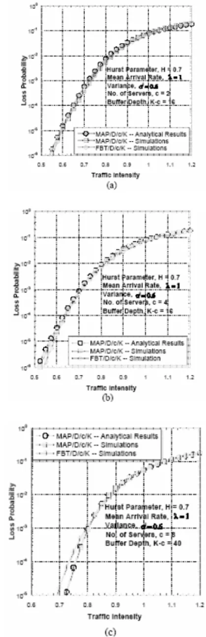
We first illustrate the loss probabilities against the traffic intensity pertaining to the analytical and the simulation results of MAP/D/c/K queues and the simulation ones of the same queues under the fractional Brownian traffic (FBT) input in Figs. 8(a)-9(c). The MAP shown in Figs. 8(a)-9(c) is obtained by fitting the FBT traffic with mean arrival rate λ = 1, variance σ2 = 0.6, and Hurst parameter H = 0.7 over a typical time-scale [10 ,10 ] 2 7 following the method proposed in [9]. From these figures, we observe that our analysis is pretty accurate.

By showing the accuracy of our analysis, we then analyze the performance of WDM OPS employing wavelength conversion under Markovian modeled self-similar traffic input, according to the related system

(22)

parameters and traffic descriptors in Figs. 9(a)-11.

Figs. 9(a) and 9(b) illustrate the comparisons of packet loss probability against the load per wavelength channel at the number of FDLs, B = 10, Hurst parameters, H = 0.7 and H = 0.9, respectively. The MAP input is obtained by emulating self-similar traffic with

λ = 1 and σ2

= 0.6 in each case. From these results, the benefit of adopting wavelength conversion is apparent when the load is moderate, i.e., employing more number of tunable wavelength channels leads to better performance. When the load is high, the advantage of employing wavelength conversion is limited.

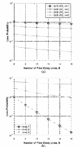
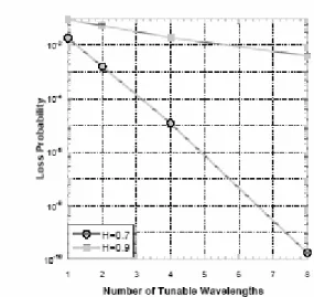
Figs. 10(a) and 10 (b) depict the comparisons of packet loss probability against the number of FDLs. The input traffic is the same as the ones in Figs. 10 (a) and 10 (b) with load set to 0.8. From these results, we observe that when H increases, the benefit of wavelength conversion becomes less prominent. We also observe that increasing the number of FDLs has limited improvement on performance. This coincides with the impact of self-similar traffic upon the storage models [34] Fig. 11 shows the comparisons of packet loss probability against the number of tunable wavelength channels when B = 10 and load per wavelength channel is 0.8 in both H = 0.7 and H = 0.9 cases. From Fig. 11, we observe that the benefit of wavelength conversion is remarkable

when the input traffic is moderate self-similar. However, this benefit decreases drastically when H increases. This is the same as the conclusions shown in [35] by simulations.

Fig. 8 Comparisons of loss probability against traffic intensity between the analytical and simulation results of MAP/D/c/K queues and the simulation ones of the same queues under FBT input, (a) c = 2 and K = 18; (b) c = 4 and K = 20; (c) c = 8 and K = 48.

(23)

Fig. 9 Packet loss probability versus channel load for a OPS with FDLs = 10, (a) H = 0.7; (b)

H = 0.9.

Fig. 10 (a) Packet loss probability versus the number of FDLs for various tunable wavelengths when the load per wavelength channel is 0.8 and H = 0:9; (b) packet loss probability versus the number of FDLs for various Hurst parameters at load per wavelength channel is 0.8 and number of tunable wavelengths is 2.

(24)

Fig. 11 Packet loss probability versus the number of tunable wavelengths for input traffic when the number of FDLs is set to be 10 and the load per wavelength is 0.8 at H = 0.7 and H = 0.9.

(3) Noncoherent Spatial/Spectral Optical CDMA System With Two-Dimensional Perfect Difference Codes

Ⅰ Introduction

Because the demand of bandwidth increases rapidly, the access network becomes the bottle neck of the internet. PON has many advantages, currently most of PONs employ Time Division Multiple Access (TDMA) techniques. However, OCDMA has many benefits such as security, flexible transmission and no need for high speed electronics devices. OCDMA has attracted a lot of attention. OCDMA PON is a promising candidates for broadband access network applications. Because of non-negative power for amplitude modulation/direct detect optical signals,

optical orthogonal codes (OOCs) are a family of (0, 1) sequences with good autocorrelation and cross correlation properties. (n,w,λa,λc) – OOCs denotes the OOCs with code length n , code weightw, autocorrelationλa and cross correlationλc. Forλa =λc =λ, we may simply the notation as (n, w,λ) – OOCs. The code sizeΦ is given by [36]

⎥ ⎦ ⎥ ⎢ ⎣ ⎢ ⎥⎦ ⎥ ⎢⎣ ⎢ − − ⎥⎦ ⎥ ⎢⎣ ⎢ − − ≤ Φ ... ... 1 1 1 λ λ w n w n w

By relaxing the cross correlation constrain, the code size of (n, w,1,2) - OOCs is about 10 times larger than that of (n, w,1) – OOCs [37]. However the bit error rate (BER) performance of the later is better than that of the former. The one-dimensional ( n,w,λa,λc ) – OOCs, which speads the input data bits in time domain, have been studied intensively. Recently the 2-D spectral/time OOCs were proposed [42]. The 2-D spectral/time OOCs can support a large number of users. The 2-D OOCs can be considered as an mxn matrix with (0, 1) elements. An example of 2-D OOCs is shown in Fig. 12 [42].

(25)

Fig. 12 An example of two (3×21, 4, 1, 1)-MWOOCs

For any codeword X= {X } of the _ij

(mxn,w,λ_a,λ_c) – OOCs. The periodic autocorrelation λ_a satisfies a m i n j f ij ijX X λ

∑∑

− = − = ⊕ ≤ 1 1 1 0

where f is the asynchronous time shift

and ⊕ represents the modulo- n addition.

For any code words X= {X } and Y= _ij

{Y }, the periodic cross correlation _ij

c λ satisfies. c m i n j f iy ijY X λ

∑∑

− = − = ⊕ ≤ 1 1 1 0

The mxn of many 2-D OOCs are constrained by certain relations [42]. The 2-D OOCs with arbitrary combination of m and n are proposed [43], where m≤ n, we have applied the proposed 2-D OOCs to the spectral/time OCDMA systems.

Another type of 2-D OCDMA systems employ multi-fibers. Therefore

the data bits are spread in the time domain and spatial domain. The partial modified prime (PMP) codes are applied in the system. Because the system can suppress the phase-induced intensity noise (PIIN), it also has very good performance [44].

Ⅱ The 2-D spectral/time OCDMA

system

The receiver structure of the 2-D spectral/time OCDMA system using Pd codes is shown in Fig. 13 [43]. We assume the system is chip synchronous among users since it is the worst case of the performance. The average photon arrival rateΣ per pulse is given by

hf pw

η

=

Σ whereη is the APD quantum efficiency,

w

p is the received optical signal power,

h is the plauck’s constant, and f is

the optical frequency. The optical signal at the output of the second hard limiter has “on” and “off” two level which are denoted by state S1andS . The photon 0 arrival rates for state S1andS are 0

Σ and zero. With the Gaussian probability density function (pdf) assumption, the output current ϕb of

the photo detector is given by [45]

2 2 2 2 ) ( 2 1 ) ( b b b e P b σ μ ϕ πσ ϕ ϕ = − −

where bE{0, 1} for state ωb, μb is the mean value of the detector output current given by

(26)

e I T e I b GTc b c s b = ( ε + / )+ / μ have G is the average APD gain, T is c

the chip time, e is the electron charge, b

I and I are the bulk and surface c

leakage currents of the APD.

Fig. 13 The receiver structure of asynchronous OCDMA systems using double optical hard limiters

The variance of the photo current, 2 b σ is expressed as e I T e I b T F G _e _c _b _c _s b ( / ) / 2 2 = ε + + σ ) 1 )( / 1 2 ( _eff eff e k G G k T = + − −

here k_eff is the APD effective ionization ratio. The variance of thermal noise is given by L c r b b K TT e R 2 2 / 2 = σ

Where K_B is the Boltzmann’s constant, r

T and R_L are the receiver noise temperature and load resistance. The threshold is set at 2 1 0 1 1 0 σ σ σ μ σ μ θ + + =

The probabilities that the desired signal

bit by the interfering user at one work and λc works are q1 and qλ which are given by mn w q c 2 2 1 λ − = and mn q _c 2 1 = λ

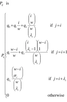
The number of code weights interfered by α interfering users can be modeled by the Markov chain [46]. The state transition occurs, when a new interfering user appears. The transition probability

ij P is ⎪ ⎪ ⎪ ⎪ ⎪ ⎪ ⎪ ⎪ ⎪ ⎩ ⎪ ⎪ ⎪ ⎪ ⎪ ⎪ ⎪ ⎪ ⎪ ⎨ ⎧ + = ⎟⎟ ⎠ ⎞ ⎜⎜ ⎝ ⎛ ⎟⎟ ⎠ ⎞ ⎜⎜ ⎝ ⎛ − + = ⎟⎟ ⎠ ⎞ ⎜⎜ ⎝ ⎛ ⎟⎟ ⎠ ⎞ ⎜⎜ ⎝ ⎛ − ⎟⎟ ⎠ ⎞ ⎜⎜ ⎝ ⎛ − + − = ⎟⎟ ⎠ ⎞ ⎜⎜ ⎝ ⎛ ⎟⎟ ⎠ ⎞ ⎜⎜ ⎝ ⎛ + + otherwise 0 if 1 if 1 1 if 1 1 0 c c c c c c ij i j w i w q i j w i w i q w i w q i j w w i q w i q q P c λ λ σ λ λ λ λ λ λ where c q q q₀ =1− ₁− _λ Let ]K(α) =[K₀(α)K₁(α)... K_w(α) represent the state probability of the Markov chain given α [44]. Let Pdemote the state transition matrix where P={P_ij} for

w j

i ≤

≤ ,

(27)

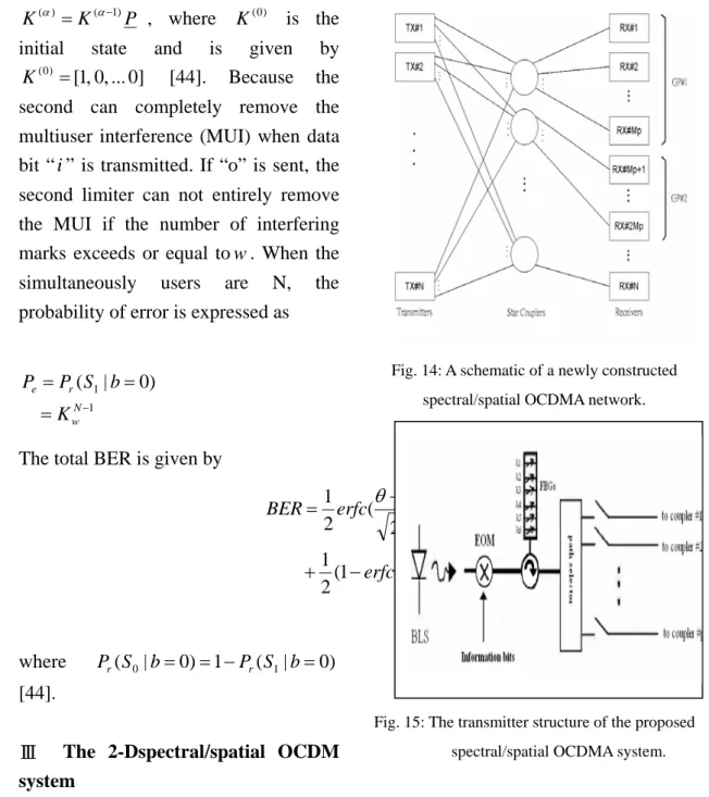
P K

K(α) = (α−1) , where K(0) is the initial state and is given by

0] ... , 0 , 1 [ ) 0 ( = K [44]. Because the

second can completely remove the multiuser interference (MUI) when data bit “i ” is transmitted. If “o” is sent, the

second limiter can not entirely remove the MUI if the number of interfering marks exceeds or equal tow. When the simultaneously users are N, the probability of error is expressed as

1 1 ) 0 | ( − = = = N w r e K b S P P

The total BER is given by

) 0 | ( )) 2 ( 1 ( 2 1 ) 2 ( 2 1 ) 0 | ( ) 2 ( 2 1 1 2 1 1 2 1 1 0 2 0 0 = − − + − + = − = b S P erfc erfc b S P erfc BER r r σ θ μ σ θ μ σ μ θ where )Pr(S0|b=0)=1−Pr(S1|b=0 [44].

Ⅲ The 2-Dspectral/spatial OCDM

system

Ⅲ-1 System Architecture

The proposed system Architecture is shown in Fig 14. The structures of the transmitter and receiver are depicted in Figs 15 and 16 [43].

Fig. 14: A schematic of a newly constructed spectral/spatial OCDMA network.

Fig. 15: The transmitter structure of the proposed spectral/spatial OCDMA system.

Fig. 16: The receiver structure of the proposed spectral/spatial OCDMA system.

寬頻光都會與接取網路之關鍵技術－總計畫:寬頻光都會與接取網路之關鍵技術(2/3)

行政院國家科學委員會專題研究計畫 期中進度報告