應用改善式啟發解與基因演算法求解晶圓針測排程問題之最大完成時間最小化

全文

(1)國立交通大學工業工程與管理學系碩士班. 碩士論文. 應用改善式啟發解與基因演算法求解晶圓針測排程問題之最大完成時間最小化 Improving Heuristics and Genetic Algorithms for Minimizing the Maximum Completion Time for the Wafer Probing Scheduling Problem (WPSP). 研. 究. 生：蔡育燐. 指導教授：彭文理博士楊明賢博士. 中華民國九十三年六月 i.

(2) 應用改善式啟發解與基因演算法求解晶圓針測排程問題之最大完成時間最小化. 研究生：蔡育燐指導教授：彭文理國立交通大學工業工程與管理學系碩士班. 博士. 摘要晶圓廠針測區排程問題(Wafer Probing Scheduling Problem, WPSP)是平行機台排程問題的實例應用，另外也可應用在積體電路(IC)製造業以及其他的工業用途。求解目標式為最小化機台總工作量之晶圓廠針測區排程問題可能會導致平行機台間負荷的不平衡，而無法被現場監控者所接受。因此，在本篇論文中我們把目標式改為最小化最大完成時間之晶圓廠針測區排程問題並用一整數規劃問題來描述之。為了有效解決晶圓針測區排程問題之最大完成時間最小化，我們提出了結合初估產能負荷及晶圓廠針測區排程問題的演算法來做重複的求解之改善式啟發解法。此外，我們還提出了不同於以往的混合式基因演算法，其使用之初始母體為晶圓廠針測區排程問題的演算法所求得的排程解與部分排程保留導向的基因交配法來對問題作排程的流程。為了有效評估兩演算法在不同問題情境下的績效，本論文使用了四種影響晶圓廠針測區排程問題之特性來產生產生多組不同的問題。測試結果發現改善式啟發解在我們所設計的問題下其平行機台排程工件之最大完工時間比混合式基因演算法來的好。且當混合式基因演算法使用改善式啟發解之排程解當作初始母體時，其在某些問題情境下還可對改善式啟發解的排程解做更進一步的改善。. 關鍵詞：晶圓針測，平行機台排程，最小化最大完成時間，改善式啟發解，基因演算法 ii.

(3) Improving Heuristics and the Hybrid Genetic Algorithm for minimizing the maximum completion time of the Wafer Probing Scheduling Problem (WPSP). Student : Yu-Lin Tsai Advisor : Dr. Wen-Lea Pearn Department of Industrial Engineering and Management National Chiao Tung University. Abstract The wafer probing scheduling problem (WPSP) is a practical version of the parallel-machine scheduling problem, which has many real-world applications including the integrated circuit (IC) manufacturing industry and other industries. WPSP carries the objective to minimize the total machine workload, which might lead to unbalanced workloads among the parallel machines and be unaccepted for the shop floor supervisors.. Therefore, we consider WPSP with the objective to minimize the. maximum completion time and formulate the WPSP with minimum makespan as an integer-programming problem.. To solve the WPSP with minimum makespan. effectively, we proposed the improving heuristics, which add the expected machine load into savings and insertion algorithms for solving problems repeatedly.. Besides,. we also provide hybrid GA including initial population by WPSP algorithms and sub-schedule preservation crossover to solve the considered problem.. To evaluate. the performance of the two proposed approaches under various conditions, the performance comparison on a set of test problems involving four problem characteristics are provided.. The computational result shows that improving. heuristics are better than hybrid GA in scheduling solutions and velocities of WPSP with minimum makespan.. When hybrid GA is using initial population by improving. heuristics, it can make further improvement for the best solution of improving heuristics in some situations.. Keyword: wafer probing, parallel-machine scheduling, minimum makespan, improving heuristics, genetic algorithms iii.

(4) Contents Abstract ........................................................................................................................ iii Contents ........................................................................................................................iv List of Tables..................................................................................................................v List of Figures ...............................................................................................................vi Notations ......................................................................................................................vii 1. Introduction................................................................................................................1 2. Problem definition and formulation...........................................................................2 3. The Improving Heuristics ..........................................................................................6 3.1 Phase I - Existing network algorithms .............................................................8 3.2 Phase II - Network Adjusting Procedure .......................................................14 4. The Genetic Algorithm For WPSP with min C max ...............................................15 4.1 GA for Parallel Machine Problem..................................................................16 4.2 The Hybrid Genetic Algorithm ......................................................................21 4.2.1 Problem encoding ...............................................................................22 4.2.2 Initialization ........................................................................................23 4.2.3 Selection..............................................................................................23 4.2.4 Genetic operators ................................................................................24 4.2.5 Elitist Strategy.....................................................................................27 4.2.6 Stopping Criteria.................................................................................28 5. Problem Design and Testing ....................................................................................28 6. Computational Results .............................................................................................32 6.1 ANOVA Analysis of Improving Heuristics....................................................32 6.2 Computational Results of GA with Initial Population from WPSP algorithms ........................................................................................................................35 6.3 Further Improvement of Hybrid GA with Initial Population from Improving Heuristics .......................................................................................................36 7. Conclusion ...............................................................................................................37 Reference .....................................................................................................................39 Appendix......................................................................................................................43. iv.

(5) List of Tables Table 1. The comparison of GA under various problem characters, crossover, and mutation. ........................................................................................................18 Table 2. Summary of 16 problem design .....................................................................31 Table 3. Computational results of WPSP algorithms in 16 test problems. ..................33 Table 4. Computational results of improving heuristics under all kinds of situations. 33 Table 5. Check of normality assumption for 96 solutions in 16 test problems............34 Table 6. The summary of ANOVA table under 99% confidential intervals.................34 Table 7. Duncan’s multiple comparisons for the performance of WPSP algorithms...34 Table 8. The comparison of hybrid GA with WPSP algorithms and improving heuristics in testing problems.........................................................................36 Table 9. Computation results of GA with initialization of improving heuristics.........37 Table A1. Processing times of jobs with product types and product families under low total processing time level...........................................................................43 Table A2. Processing times of jobs with product types and product families under high total processing time level...........................................................................43 Table A3. Tightness of due dates in 16 testing problems.............................................43 Table A4. All jobs with product types and due dates while tightness of due dates is stable and total processing time level is low................................................44 Table A5. All jobs with product types and due dates while tightness of due dates is increasing and total processing time level is low. .......................................44 Table A6. All jobs with product types and due dates while tightness of due dates is stable and total processing time level is high. .............................................44 Table A7. All jobs with product types and due dates while tightness of due dates is increasing and total processing time level is high. ......................................45 Table A8. Setup time with product types while product family ratio is 2 and temperature changing is not considered. .....................................................45 Table A9. Setup time with product types while product family ratio is 2 and temperature changing is considered. ...........................................................46 Table A10. Setup time with product types while product family ratio is 6 and temperature changing is not considered. ...................................................46 Table A11. Setup time with product types while product family ratio is 6 and temperature changing is considered...........................................................47. v.

(6) List of Figures Figure 1. The structure of the improving heuristic ........................................................7 Figure 2. The flowchart of the execution for hybrid genetic algorithm.......................22 Figure 3. Copy the partitioning structure to offspring .................................................25 Figure 4. Copy the sub-schedules to offspring ............................................................26 Figure 5. Fill the empty of the offspring from the other parent...................................26 Figure 6. Illustration of swapping technique ...............................................................27 Figure 7. The trend of average solutions in population of hybrid GA repeated four times in problem No. 7..................................................................................47 Figure 8. The trend of best solution in population of hybrid GA repeated four times in problem No. 7. ..............................................................................................48 Figure 9. The trend of average solutions in population of hybrid GA repeated four times in problem No. 8..................................................................................48 Figure 10. The trend of average solutions in population of hybrid GA repeated four times in problem No. 8................................................................................49 Figure 11. The further improvement of hybrid GA with initialization by improving heuristics in problem No. 8.........................................................................49 Figure 12. The further improvement of hybrid GA with initialization by improving heuristics in problem No. 16.......................................................................50. vi.

(7) Notations IP modeling Rj. : the jth product type of jobs. Ij. : the number of jobs in jth product type of jobs. mk. : the kth machine of identical parallel machines. ri. : the job of WPSP with minimum makespan. F. : the total number of product families. J. : the total number of product types. Jf. : the total number of product types in product family f. Rj. : the jth subset (product type) of jobs to be processed. C max. : the maximum completion time (makespan). W. : the predetermined machine capacity expressed in terms of processing time units. s ii ′. : the sequentially dependent setup time between any two consecutive jobs. ri and ri′ xik. : the variable indicating whether the job ri is scheduled on machine mk. pi. : the processing time of job ri in cluster R j ( ri ∈ R j ). tik. : the starting time of job ri to be processed on machine mk. bi. : the ready time of job ri. di. : the due date of job ri. ei. : the latest starting processing time of job ri. yii′k. : the precedence variable, which should be set to 1 if the two jobs ri and. ri′ are scheduled on machine mk and job ri precedes job ri′ (not necessarily directly), and 0 otherwise. z ii′k. : the direct-precedence variable, which should be set to 1 if the two jobs. ri and ri′ are scheduled on machine mk and job ri precedes job ri′ directly, and 0 otherwise. Q. : a constant, which is chosen to be sufficiently large enough to make constraints of IP model satisfied. Improving Heuristics Max[ s Ui ] : the maximal setup time of machine switching from idle status (denoted by the label “U”) to processing status. Max[ siU ] : the maximal setup time of machine switching from processing status to vii.

(8) idle status. Max1[ sii′ ] : the maximal setup time of two consecutive jobs processed on machine coming from different product type and different product family. Max2[ sii′ ] : the maximal setup time of two consecutive jobs from different product type and same product family. σ. : the parameter which may vary according to the problem data structure used in estimation of expected machine load. ES. : the sum of expected setup time on identical parallel machines. EL. : the expected machine workload. iνk. : the selected job has been scheduled on the ν th position of machine mk. SAii′. : the saving value for any pairs of jobs ri and ri′ , and U denotes the idle status. MSAii'. : the modified saving value for any pairs of jobs ri and ri′ , and U denotes the idle status. A. : the parameter added into the savings function of modified sequential saving (MSA) to present the percentage of postponement restriction. B. : the parameter added into the savings function of modified sequential saving (MSA) to present the percentage of time window restriction. c1 (u , k ,ν ) : the insertion cost of job u added into the ν th position on machine mk. in sequential insertion (SIA). c1′ (u, k ,ν ) : the best insertion cost of job u added into the ν * th position on *. machine mk in sequential insertion (SIA) c 2 (u ). c′2 (u ). : the regret value of job u in sequential insertion (SIA). *. : the largest regret value among all unscheduled jobs in sequential. insertion (SIA) c1′′(u,k * ,ν* ) : the best insertion cost of job u added into the ν * th position on. c3 (u ). c3′ (u * ). machine mk * in parallel insertion (PIA) : the regret value of job u in parallel insertion (PIA) : the largest regret value of job u * among all unscheduled jobs in parallel insertion (PIA). c11 (u , k ,ν ) : the modified insertion cost of job u added into the ν th position on. machine mk in parallel insertion with the slackness (PIA II). λ. : the parameter which represents the ratio of the insertion values that the slackness would have in parallel insertion with the slackness (PIA II). viii.

(9) c4 (u ). : the modified regret value of job u in parallel insertion with the variance of regret measure (PIA IV). Var (c1′ ). : the variance of best insertion cost between all parallel machines in parallel insertion with the variance of regret measure (PIA IV). Avg (c1′ ). : the average value of best insertion cost on all identical parallel machines in parallel insertion with the variance of regret measure (PIA IV). ϕ. : the parameter which determines the schedule ranking of all jobs on all identical parallel machines in parallel insertion with the variance of regret measure (PIA IV). LB. : lower bound of the adjusting procedure. UB. : upper bound of the adjusting procedure. MLk. : the total machine load on machine mk. δ. : the repeat times of executing WPSP algorithms in improving heuristics. Hybrid GA C maxα ,β : the makespan of the α th chromosome in the pool when the GA cycle proceeds to the β th generation K. : the available machine number of identical parallel machines. F (α , β ). : the fitness value of the α th chromosome in the pool when the GA cycle proceeds to the β th generation. dνk. : the due date of job on ν th position of machine mk. SSLνnk. : the sum of slackness values for n consecutive jobs on machine mk , which are located from ν th to (ν + n − 1) th position. SSLνnk. : the average value of slackness for n jobs started from ν th to (ν + n − 1) th position on machine mk. n. : the number of job consideration on machine mk while estimating the slackness of job combinations. Nk. : the number of jobs on machine mk. R. : the product family ratio in testing problems. TI (Y ). : the tightness value of jobs before Yth due date point. P (Y ). : the total processing time of jobs of which due dates are given before Yth due date point. Cap(Y ). : the available capacity of machine before Yth due date point. Num(Y ). : the number of jobs of which due dates are given before Yth due date point. ix.

(10) 1. Introduction The wafer probing scheduling problem (WPSP) [1,2] is a practical version of the parallel-machine scheduling problem, which has many real-world applications, especially in the integrated circuit (IC) manufacturing industry. There are wafer fabrication, wafer sorting, assembly, and final test in the processes of IC product, and the first and fourth stages are related processes, where the testers are expensive and critical. Pearn et al. [2] considered the wafer probing scheduling problem (WPSP) with the objective of minimizing total workload. They formulated the WPSP as an integer programming problem and transformed the WPSP into the vehicle routing problem with time window (VRPTW).. They provided three VRPTW algorithms for. solving the WPSP and their computational results showed that the network transformation of identical parallel machine scheduling was efficient and applicable under. the. objective. of. raising. identical. parallel. machine. utilities.. A. minimizing-makespan schedule not only can result in higher efficiency and resource utilization but minimize the time, which jobs are operating in the factory.. The. identical parallel-machine scheduling problem with minimized makespan also identifies the bottleneck machine, which needs to be arranged carefully. This paper considers the identical parallel-machine scheduling problem with minimizing makespan, which has been proved to be a NP problem [3,4]. In view of the NP-hard nature of the problem, several polynomial time algorithms have been proposed for its solution. It has been traditional solved by operational methods such as integer programming, branch and bound method, dynamic programming, etc.[5-9]. Min et al. [10] proposed a genetic algorithm, which contains the procedures of coding, initializing, reproducing, crossover, and mutation. It was actually efficient for large scale problems.. Besides, Gupta et al. [11] provided a LISTFIT algorithm, or the. SPT/LPT and MULTIFIT procedure, for solving parallel-machine scheduling problems with minimizing makespan. Some proposed algorithms also have been used for solving parallel-machine scheduling with other objectives. Azizoglu and Kirca [12] proposed a branch and bound algorithm combined with lower bounding. 1.

(11) scheme for the objective of minimizing total tardiness.. Lee and pinedo [13]. presented a three phases algorithm incorporating the ATCS rule and simulated annealing method for minimizing the sum of weighted tardiness and the experimental results showed that simulated annealing method had a great improvement of solutions. Park, Kim, and Lee [14] addressed an extension of the ATCS (Apparent Tardiness Cost with Setups) rule for the objective of minimizing total weighted tardiness. Hurkens et al. [15] proposed a 0-1 interchange, which is the procedure of the job moving iteratively to the machine with minimal load if its processing time is less than the difference between maximum and minimum machine load. Veen et al. [16] formulated an integer programming by dividing jobs into K job-classes and considered that the change-over time between two consecutive jobs is dependent on the job-class to which the two jobs belonged. For the WPSP with the objective of minimizing makespan, we first formulate our problem as an integer programming, which includes job due dates, job processing times, job sequence-dependent setup time, and machine capacities. In section 3, we propose improving heuristics, which are the network algorithms merging with two different adjusting procedures respectively, for making the local optimum closer to global one. In section 4, we address a hybrid genetic algorithm in contrast to the two-phase heuristics we developed before. In the last section, we will describe the experimental framework and present the analysis of the results by comparing the genetic algorithm with two-phase heuristics.. 2. Problem definition and formulation Consider several product types of jobs with ready time and due date to be processed on identical parallel machines with capacity constraint. The job processing time depends on the product type of the job processed. Setup times for two consecutive jobs of different product type are sequence dependent. The objective is to find a schedule for the jobs which minimizes the maximum completion time without violating the due date restrictions and the machine capacity constraints. We first define R = {R1 , R2 ,K, RJ , RJ +1 } as the J + 1 subsets (product types) of 2.

(12) jobs to be processed with each subset R j = {ri | i = I j −1 + 1, I j −1 + 2,K, I j −1 + I j }. {. containing I j jobs, where I 0 =0 and I J +1 =K. Thus, job subset R1 = r1 , r2 , K, rI1 contains. {. I1. jobs,. RJ +1 = rI J +1 , rI J +2 ,K, rI J + K. {. R2 = rI1 +1 , rI1 + 2 ,K, rI1 + I 2. } contains. }. contains. I2. jobs,. I J +1 (K) jobs, where I1 + I 2 + ... + I J = I .. }. and Let. F be the total number of product families and J f be the total number of product. types in product family f , where. F. ∑J f =1. f. =J.. Then M = {m1 , m2 ,K, mk } can be. defined as the set of machines containing K identical machines. The job subset RJ +1 , which is a pseudo product type including K jobs, is used to indicate the K machines are in idle state.. Therefore, there are I+K jobs grouped into J + 1. product types, at where the first I jobs are divided into J product types and the last K jobs are pseudo jobs. Let pi be the processing time of job ri in cluster R j. ( ri ∈ R j ). Since the job processing time depends on the product type of the job, then pi should be equal to p J (i ) given the function J (i ) representing the product type of job ri . Let C max be the maximum completion time (makespan) and W be the predetermined machine capacity expressed in terms of processing time units respectively. Let sii′ be the sequentially dependent setup time between any two consecutive jobs ri and ri′ , in which sii′ is equal to s J ( i ) J ( i ' ) . Further, let x ik be the variable indicating whether the job ri is scheduled on machine mk .. If job ri should be processed on machine mk , set x ik = 1 ,. otherwise set x ik = 0 .. Let tik be the starting time of job ri to be processed on. machine mk . Set bi as the ready time of job ri and d i as the due date of job ri . The starting processing time tik should not be greater than the latest starting processing time ei , which relates to the due date d i and can be computed as ei = d i − p i .. The starting processing time tik also should not be less than the. earliest starting processing time bi . If job ri is ready to be processed initially, then set bi to 0.. We note that the processing time and due dates for the job in RJ +1. should be set to 0 so that these pseudo jobs can be scheduled as the first jobs on each machine, which indicate that each machine is initially in idle state. Let y ii′k be the precedence variable, where y ii′k should be set to 1 if the two jobs ri and ri′ are scheduled on machine mk and job ri precedes job ri′ (not necessarily directly), and where y ii′k = 0 otherwise. Further, let z ii′k be the direct-precedence variable, 3.

(13) where z ii′k should be set to 1 if the two jobs ri and ri′ are scheduled on machine mk and job ri precedes job ri′ directly, and where z ii′k = 0 otherwise. To find a schedule for these jobs which minimizes makespan without violating the machine capacity and due date constraints, we consider the following integer programming model: Minimize C max subject to K. ∑ x ik = 1, for all i. (1). k =1. I +K. ∑ x ik = 1, for all k. (2). i = I +1 I +K. I +K I +K. i =1. i =1. i′ =1. I +K. I +K. I +K. i =1. i =1. i ′ =1. ∑ xik pi + ∑ ( ∑ z ii′k sii′ ) ≤ C max, for all k. (3). ∑ x ik p i + ∑ ( ∑ z ii′k s ii′ ) ≤ W , for all k. (4). t ik + p i + s ii′ − t i′k + Q( y ii′k − 1) ≤ 0, for all i, k. (5). t ik + p i + s ii′ − t i′k + Q( y ii′k + z ii′k − 2) ≥ 0, for all i, k. (6). t ik ≥ bi x ik , for all i, k. (7). t ik ≤ ei x ik , for all i, k. (8). ( y ii′k + y i′ik ) − Q( x ik + x i′k − 2) ≥ 1, for all i, k. (9). ( y ii′k + y i′ik ) + Q( x ik + x i′k − 2) ≤ 1, for all i, k. (10). ( y ii′k + y i′ik ) − Q( x ik + x i′k ) ≤ 0, for all i, k. (11). ( y ii′k + y i′ik ) − Q( x i′k − x ik + 1) ≤ 0, for all i, k. (12). ( y ii′k + y i′ik ) − Q( x ik − x i′k + 1) ≤ 0, for all i, k. (13). y ii′k ≥ z ii′k for all i, k. (14). I +K. ∑ x ik − ∑ z ii′k = 1, for all k. (15). y ii*k + z ii*k − Q( y ii*k + z ii*k − 2) − Q( y ii′k − z ii′k − 1) ≥ 2, for all i, k. (16). x ik ∈ {0,1}, for all i, k. (17). y ii′k ∈ {0,1}, for all i, k. (18). i =1. i ≠i′. 4.

(14) z ii′k ∈ {0,1}, for all i, k. (19). The constraints in (1) guarantee that job ri is processed by one machine exactly once. The constraints in (2) guarantee that only one pseudo job ri , I + 1 ≤ i ≤ I + K , is scheduled on a machine. The constraints in (3) state that each machine workload does not exceed the maximum completion time C max among all K machines. The constraints in (4) state that each machine workload does not exceed the machine capacity W . The constraints in (5) and (6) ensure that t ik + p i + s ii′ = t i′k if job ri precedes job ri′ directly ( y ii′k = 1 and z ii′k = 1 ). The constraints in (5) ensure the satisfaction of the inequality t ik + p i + s ii′ ≤ t i′k. if job ri preceding job ri′. ( y ii′k = 1). The number Q is a constant, which is chosen to be sufficiently large so that the constraints in (5) are satisfied for y ii′k = 0 or 1 . For example, we can choose. Q = ∑iI=1 ( p i + max i′ {s ii′ }) .. The constraints in (6) ensure the satisfaction of the. inequality t ik + pi + sii ' ≥ t i 'k and the event the jobs ri proceeding job ri′ directly ( yii 'k + z ii 'k − 2 = 0 ). The constraints in (7) and (8) state that the starting processing time t ik for each job ri scheduled on machine mk ( xik = 1 ) should not be less than the earliest starting processing time bi and not be greater than the latest starting processing time ei. The constraints in (9) and (10) ensure that one job should precede another ( yii 'k +. y i 'ik = 1) if two jobs are scheduled on the same machine ( xik + xi 'k - 2 = 0). The number Q is a constant, which is chosen to be sufficiently large so that the constraints in (9) and (10) are satisfied for xik + xi 'k - 2 < 0. The constraints in (11) ensure that the precedence variables yii 'k and y i 'ik should be set to zero ( yii 'k + y i 'ik ≤ 0) if any two jobs ri and ri′ are not scheduled on the machine mk ( xik + xi 'k = 0). The constraints in (12) and (13) ensure that the precedence variables yii 'k and y i 'ik should be set to zero ( yii 'k + y i 'ik ≤ 0) if any one job ri or ri′ is not scheduled on the machine mk . The constraints in (12) indicates the case that job ri is scheduled on machine mk and the job ri′ is scheduled on another machine ( xi 'k - xik + 1 = 0) and the constraints in (13) indicates the case that job ri′ is scheduled on machine mk and the job ri is scheduled on another machine ( xik - xi 'k + 1 = 0). The constraints in (14) ensure that job ri could precede job ri′ directly ( z ii 'k = 1) 5.

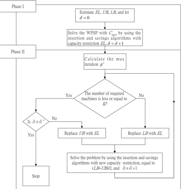
(15) only when yii 'k = 1 and job ri could not precede job ri′ directly ( z ii 'k = 0) if job ri is scheduled after job ri′ ( yii 'k = 0). The constraints in (15) state that there should exist I-1 directly precedence variables, which are set to 1 on the schedule with I jobs. The constraints in (16) state that when the job ri precedes job ri′ but not consecutively ( yii 'k = 1 and z ii 'k = 0), then there must exist another job ri* scheduling after job ri directly ( yii*k = 1 and z ii*k = 1 ) and ensuring the satisfaction of the inequality yii*k + z ii*k ≥ 2 .. 3. The Improving Heuristics There are many kinds of network algorithms for WPSP with minimizing total machine workload.. VRPTW algorithms are one of them which have been. successfully applied to solve WPSP with good efficiency.. Because VRPTW. algorithms are effective for solving WPSP, we adopt these WPSP algorithms to solve WPSP with minimum makespan in the following of this paper.. We use these. algorithms based on expected machine load EL restriction to find feasible solutions of WPSP with minimum makespan in phase I of improving heuristics. Then feasible solutions would be improved through the adjusting procedure, phase II of improving heuristics. In this paper we propose two-phase heuristics, improving heuristics, to help solving the WPSP with minimum makespan more efficiently. The main idea is that improving heuristics use the adjusting procedure to improve feasible solutions solved by WPSP algorithms.. The improving procedure would search the best. solution through the different machine workload repeatedly.. Phase one of the. improving heuristic is to apply some efficient WPSP algorithms based on the expected machine load EL restriction for finding feasible solutions of WPSP with minimum makespan.. In phase two, we will provide an improving procedure for making the. local optimum solved by WPSP algorithms climbing to the global one. The structure of the improving heuristic is shown as Fig. 1.. 6.

(16) Phase I Estimate EL, UB, LB, and let δ =0 Solve the WPSP with Cmax by using the insertion and savings algorithms with capacity restriction EL, δ = δ + 1. Phase II Calculate the max iteration δ *. Yes. Is δ>δ*. The number of required machines is less or equal to K?. No. Replace UB with EL. Yes. No. Replace LB with EL. Solve the problem by using the insertion and savings algorithms with new capacity restriction, equal to (LB+UB)/2, and δ=δ+1. Stop. Figure 1. The structure of the improving heuristic To find the minimal C max more efficiently, we provide the estimation of the expected machine workload EL corresponding to the parallel machine scheduling problem, which will be utilized along with scheduling algorithms.. Before. calculating EL , we would define the notation ES, which is the total expected setup time of all identical parallel machines. The expected machine workload EL equals to the sum of the expected setup time ES and the total job processing time divided by the number of available machines K. Let sii′ be the sequence dependent setup time of any two consecutive jobs ri and ri′ on the same machine. Let Max[ s Ui ] be the maximal setup time of machine switching from idle status (denoted by the label “U”) to processing status, Max[ siU ] be the maximal setup time of machine switching from. 7.

(17) processing status to idle status, Max1[ sii′ ] be the maximal setup time of two consecutive jobs processed on machine coming from different product type and different product family, Max2[ sii′ ] be the maximal setup time of two consecutive jobs from different product type and same product family. Therefore, equation (20) expresses the computation of ES . F. ES = K × ( Max[ s Ui ] + Max[ siU ] + ( F. + Max 2[ sii′ ] ×. F. Jf 2. ∑P. f =1 J 2. P + C1J. + 0×. ∑C. f =1 J 2. I − 1) × ( Max1[ sii′ ] × K. J. J. ∑ C 1 f × ( J − C1 f ). f =1. P2J + C1J. (20). Jf 1. P + C1J. )). where the notations “P” and “C” in equation (20) represent the symbol of permutation in statistics. And the coefficient “0” indicates the setup time of two consecutive jobs from the same product type and the same product family should be zero. Let the parameter σ , which may vary according to the problem data structure, be the allowance of uniform capacity decided by the user and be set as the value between -0.5 and 0.5.. We consider the expected capacity EL is the allowance multiplied by. the outcome, which is the sum of total job processing times plus the expected setup time ES divided by K machines fairly. Then we can get the EL as follows: I ⎡1 ⎤ EL = ⎢ × ⎛⎜ ∑ pi + ES ⎞⎟⎥ × (1 + σ ) ⎠⎦ ⎣ K ⎝ i =1. and − 0.5 ≤ σ ≤ 0.5. (21). 3.1 Phase I - Existing network algorithms. Generally speaking, the WPSP algorithms include insertion and saving algorithms. The insertion algorithms generally include two types, the sequential and the parallel. The saving based procedures include four types, the sequential, the parallel, the generalized,. and. the. matching. based.. We. first. define. the. order. (i0 k , i1k , ... , i( ν −1 )k , iνk , ... , iUk ) where i0 k and iUk both represent the machine mk is in the idle state, and iνk represents that selected job has been scheduled on the ν th position of machine mk . Then we would review savings and insertion algorithms 8.

(18) by citing Clark and Wright [17], Golden [18], Pearn et al. [19], Solomon [20], Potvin and Rousseau [21], and Yang et al. [22].. These algorithms are including the. sequential saving algorithm, the modified sequential saving algorithm, the sequential insertion algorithm, the parallel insertion algorithm, and modified parallel insertion algorithms. The procedures of these algorithms above are introduced as follows. Sequential savings algorithm (SSA) First of all, the sequential savings algorithm calculates the savings of all paired-jobs and creates a saving list by arranging their saving values in descending order. Then we pick the first pair of jobs from the top of the saving list to start an initial schedule. We can confirm whether a selected pair of jobs is feasible by checking the machine capacity constraint and the due date restrictions of jobs.. The sequential savings. algorithm spreads out the schedule by finding the feasible pair of jobs from the top of the savings list and adding it to either one endpoint of the schedule. If the current schedule is too tight to add any job in, choose the feasible pair of jobs from the top of the saving list as a new schedule.. Repeat this step until all jobs are scheduled.. The procedure is presented in the following. Step 1. (Initialization) Calculate the savings value SAii′ defined as the following for all pairs of jobs ri and ri′ , where U denotes the idle status.. SAii′ = s Ui + siU + sUi' + si′U -( s Ui + sii' + si′U ) = siU + sUi′ − sii′. (22). Step 2. Arrange the savings and create a list of the saving values in a descending order. Step 3. Choose the first pair of jobs from the saving list as an initial schedule. Start from the top of the savings list, and proceed with the following sub-steps: Step 3-1. Select the first pair from the top saving list without violating the machine capacity and due date constraints. Then add it to either one end of the current schedule. Step 3-2. If the current schedule is too tight to add any job on it, choose the best feasible pair on the saving list to start a new schedule. Step 4. The chosen jobs then form a feasible machine schedule. Repeat step 3 until all the jobs on the saving list are scheduled.. 9.

(19) Modified sequential savings algorithm (MSSA) The modified sequential savings algorithm adds two terms into the savings estimation, the consideration of the postponement and the time window restriction. For the postponement, the selecting way would tend to choose the pair of jobs with not only higher saving values but longer processing time. By this way, the jobs with longer processing time are forced to be processed earlier than others with shorter one. Considering the other term, the job with earlier job latest starting time ei would be placed before the job with later one e j on the savings list.. Two parameters, A and. B, are added into the savings function to present the percentage of postponement and time window restriction, and W is the predetermined capacity.. The new savings. function is expressed in the following: MSAii' = A( siU + s Ui′ − sii′ ) + (1 − A) pi + W (. B (1 − B) − ), 0 < A < 1, 0 < B < 1 ei ei′. (23). Sequential insertion algorithm (SIA) The main part of the sequential insertion is to build one schedule once until all jobs are scheduled. The sequential insertion would find the maximal benefit among the schedule places that a selected job can insert into. When the existing schedule is full of jobs, we create another new machine schedule. The initial rule is to select a job with the maximal initial setup time.. After initializing the current schedule, the. priority of selecting job depends on the regret value c2 (u ) of all unscheduled jobs. Find the best insertion place c1′ (u, k ,ν * ) of all unscheduled jobs and select job u * with the largest regret value c′2 (u * ) as the first inserted job.. The evaluations of. insertion cost and regret values are defined as follows. c1 (u , k ,ν ) = c1 (i(ν −1) k , u , iνk ) = si(ν −1) k u + suiνk − si(ν −1) k iνk. (24). c1′ (u,k,ν* ) = min[c1 (u,k,ν)]. (25). c2 (u ) = s Uu − c1′ (u,k,ν* ). (26). ν. 10.

(20) c2′ (u * ) = max[c2 (u )]. (27). u. In equation (24), the jobs i(ν −1) k and iνk are placed individually on the (ν − 1 )th and ν th positions of machine mk .. And the term s Uu of equation (26) represents. the initial setup time of the unscheduled job ru . For each unscheduled job, we first compute its best feasible insertion place c1′ (u,k,ν* ) in equation (25), and we can get the regret value of c2 (u ) in equation (26). The job with larger value c2 (u ) should have the priority to be scheduled. Therefore, select the job u * with largest value c′2 (u * ) and insert it into the best position of the schedule. All unscheduled jobs will be inserted under the following procedure. Step 1. Initialize the schedule by selecting the job with the maximal initial setup time. Step 2. For each unscheduled job, compute the best feasible insertion place ν * , which has the smallest insertion value c1′ (u,k,ν* ) on machine mk . Step 3. Select the unscheduled job u * with the largest value c2 (u * ) and put it into the best insertion place of the schedule. If the existing schedule is too full to add any unscheduled job, create a new schedule on another machine. Step 4. Repeat Step 2 and Step 3 until all jobs are scheduled. Parallel insertion algorithm (PIA) The parallel insertion algorithm constructs a set of initial schedules on all machines in the beginning. Besides, it also creates a new regret measure, which is the sum of absolute differences between the best alternative on one machine and other alternatives on other machines. A large regret measure means that there is a large gap between the best insertion place of the unscheduled job on one machine and its best insertion place on the other machines. Hence, unscheduled jobs with larger regret values should be inserted into the schedule first, because there are large cost differences of the best insertion place and second alternative. In this algorithm, we add two criteria into our selecting rule. One is the value c1′′(u,k * ,ν* ) , which has the smallest insertion cost on ν * th position of machine k * . The other is the regret value c3 (u ) different from c2 (u ) of equation (26). The insertion functions are as follows.. 11.

(21) c1′′(u,k * ,ν* ) = min[c1′ (u,k,ν * )]. (28). c3 (u ) = ∑ [c1′ (u,k,ν* ) − c1′′(u,k * ,ν* )] *. (29). c3′ (u * ) = max[c3 (u )]. (30). k. k ≠k. u. Initialization is done by selecting the unscheduled jobs with the first K largest initial setup times and putting them into the initial schedule of each machine. By applying this method, we can get the K initial schedules and compute the best insertion place in each of the schedules for all unscheduled jobs. Then we compute the regret value c3 (u ) of all unscheduled jobs and find the largest value c3′ (u * ) of job u * . Select job u * and insert it into the best position ν * of machine k * with value c1′′(u,k * ,ν* ) . The procedure of PIA is described as below. Step 1. Initialize the schedule on each machine by selecting K jobs with the first K largest initial setup times. Step 2. For each unscheduled job, find its best feasible insertion place by computing c1′′(u,k * ,ν* ) . Step 3. Calculate the regret value c3 (u ) for each unscheduled job. Select the job u * with the largest regret measure c3′ (u * ) among all unscheduled jobs. Insert it into the ν * th position of machine k * without violating the machine capacity and its due date restrictions. Step 4. Repeat Step 2 and Step 3 until all jobs are scheduled. Parallel insertion with new initial criteria (PIA I) According to idea of the VRPTW, PIA first selects the farthest node to visit at the beginning stage.. However, selecting the job with largest initial setup time, the. farthest node, may not reduce the total machine workload. Comparing to PIA, this modified one adds new initial criteria in find initial jobs of parallel machines. Inserting a job into the existing schedule of the same product family can significantly reduce the increased setup time. Because the jobs of the same product type must belong to the same family, this procedure chooses the product type including the maximal number of jobs and picks the job with the smallest latest starting time ei of this type to be the initial schedule on each machine. Once the job ri of product. 12.

(22) type J (i ) is selected for a specific machine, other jobs of product type J (i ) cannot be selected as the initial schedules on other machines. After initializing K schedules of machines, the following steps of PIA I are identical to PIA. Parallel insertion with the slackness (PIA II) In order to express the impact of job due date, this algorithm adopts the modified insertion functions c11 (u , k ,ν ) of equation (31) instead of the value c1 (u , k ,ν ) of PIA. It adds the latest starting time eu of unscheduled job u into consideration and that would make the selection rule choose the job with smaller latest starting time as the priority possibly. The modified insertion function is as the following. c11 (u , k ,ν ) = λ ( si(ν −1) k u + suiνk − si(ν −1) k iνk ) + (1 − λ )(eu ) , 0 ≤ λ ≤ 1. (31). According to the insertion function above, we can determine the ratio of the insertion values that the slackness would have by revising the value λ .. The. insertion procedure is the same as PIA. Parallel insertion with new initial criteria and slackness (PIA III) Because PIA I and PIA II do have the advantage of reducing total machine setup time, we generate the new modified parallel insertion algorithm by combining two insertion criteria of job selection. At the beginning of inserting initial jobs, the algorithm selects the product type including the maximal number of jobs and chooses the job with the smallest value ei in this product type as the initial schedule on each machine. Once the job ri of product type J (i ) is selected for a specific machine, other jobs of product type J (i ) cannot be put as the initial schedule on other machines. The insertion cost is the same as c11 (u , k ,ν ) in equation (31) and other steps in this modification algorithm are identical to PIA II. Parallel insertion with the variance of regret measure (PIA IV) The original parallel insertion procedure does not consider the impact of the. 13.

(23) variance between the best insertion places on all machines. This modified algorithm creates a new regret measure including not only the absolute total differences of the best insertion value and other alternatives but also the variance among them. Therefore, the selected job would have a significant variance Var (c1 ) under large regret values. The modified calculation of the regret value is the following. c4 (u ) = ϕ ∑ [c1′ (u,k,ν* ) − c1′′(u,k * ,ν* )] + (1 − ϕ )Var (c1 ) , 0 ≤ ϕ ≤ 1 * k ≠k. (32). K. Var (c1′ ) = [ ∑ (c1′ (u,k,ν* ) − Avg (c1 )) 2 ]( K − 1) −1 k =1. (33). K. Avg (c1′ ) = [ ∑ c1′ (u,k,ν* )]K −1. (34). k =1. The notation Var (c1′ ) in equation (33) is the variance of best insertion cost between all parallel machines, and Avg (c1′ ) is the average value of best insertion cost on all parallel machines. We can determine the schedule ranking of all jobs on all parallel machines by adjusting the parameter ϕ . 3.2 Phase II - Network Adjusting Procedure. In accordance with WPSP with minimum makespan, we develop an adjusting procedure for WPSP algorithms. The adjusting procedure is proceeding based on the concept of lower bound LB and upper bound UB constraints.. The adjusting. procedure is searching a near-optimal solution under the lower bound and upper bound, so the solution time of the adjusting procedure is longer than Phase I. Here are the steps of the adjusting procedure we developed. Adjusting Procedure The procedure makes the basic solutions solved by phase I closer to the optimum based on lower bound and upper bound restriction. Let MLk be the total machine load on machine mk , and let δ be the number of adjusting expected machine load EL .. Here comes the detail of the adjusting procedure.. Step 1. Let δ be zero and set the value EL0 be the same of EL . Use the WPSP algorithm described to generate a basic solution by adding a restriction of 14.

(24) capacity EL0 into it. Step 2. Here we define the initial lower bound and upper bound as follows.. LB 0 = min{MLk }. (35). k∈K. UB 0 = max{ MLk } + max{ pi } k∈K. (36). i∈I. According to the property of the solution, we define the maximal number δ * of adjusting in two ways. (1) If the actually required number of machines k is smaller than the number of available machines K , we let δ * = log 2 ( EL0 − LB 0 ) , which represents the maximal adjusting times we can use in this adjusting procedure. (2) If the actually required number of machines k is larger than the number of available machines K , we let δ * = log 2 (UB 0 − EL0 ) in another way. Step 3. The step is divided into two different decision rules. (1) If the actually required number of machines k is smaller than the number of available machines K , set the value UB δ to be the same of ELδ , and update δ with the increment 1. The expected machine load is replaced with ( LB δ ′ +UB δ ′ ) / 2 , where δ ′ = δ − 1 , that is, ELδ = ( LB δ ′ + UB δ ′ ) / 2 . (2) If the actually required number of machines k is larger than the number of available machines K , set the value LB δ to be the same of ELδ , and update δ with the increment 1. The expected machine load is replaced with ( LB δ ′ +UB δ ′ ) / 2 , where δ ′ = δ − 1 . The adjusting equation is the same as the one above. Step 4. Restart the network algorithm with the restriction of adjusting value ELδ . Step 5. If the value of δ is larger than δ * and the δ th scheduling solution is feasible, stop the procedure. Otherwise ( δ is less than δ * or the δ th scheduling solution is infeasible) go to step 3 until all jobs are scheduled.. 4. The Genetic Algorithm for WPSP with min C max A genetic algorithm is a search algorithm based on the mechanism of genetics and evolution, which combines the exploitation of past results with the information of new areas of the search space. A genetic algorithm can imitate some innovative talent of a human search by using the surviving techniques of fitness function.. The. mechanism of a genetic algorithm is very simple, involving nothing but copying strings and swapping positions among strings. In every new generation of a genetic algorithm, a set of strings are created exploiting information from the previous ones. With this collection of artificial strings, a new part of population is tried for good measure and the best overall solution would become the candidate solution to the 15.

(25) problem. 4.1 GA for Parallel Machine Problem. The genetic algorithm takes advantage of historical information effectively to proceed with new search points for expected improvement. Simple operation and effective power are two primary attractions of the GA approach. The effectiveness of GA depends on an appropriate mix of exploration and exploitation. Two genetic operators, crossover, and mutation, are designed to approach this goal.. Many. researchers have considered the parallel-machine scheduling problem by using the genetic approach. Zomaya and Teh [23] employed a GA considering load balancing issues suchlike threshold policies, information exchange criteria, and inter-processor communication, to solve the dynamic load balancing problem with minimizing the maximum completion time.. Cheng et al. [24,27] considered an identical parallel. machine system with an objective of minimizing the maximal weighted absolute lateness and proposed a hybrid algorithm which combined the GA with the due date determination. They proved that mutation should play more critical role than the crossover and the hybrid genetic algorithm did outperform the conventional heuristics. Min and Cheng [25] provided a genetic algorithm based on the machine code for minimizing makespan in identical parallel machine scheduling problem and it was fit for larger scale problems with comparison to LPT and SA. Cochran et al. [26] proposed a two-stage multi-population genetic algorithm (MPGA) to solve parallel machine with multiple objectives.. Multiple objectives are combined via the. multiplication of the relative measure of each objective in the first stage, and the solutions of the first stage are arranged into sub-population to evolve separately under the elitist strategy.. Ulusoy et al. [28] proposed a genetic algorithm with the. crossover operator MCUOX for solving the parallel-machine scheduling problem with minimizing the total weighted earliness and tardiness values. They showed that GA with MCUOX outperformed in larger-sized, more difficult problems. Herrmann [29] provided a two-space genetic algorithm representing solutions and scenarios for solving minimizing makespan problems and the experiment showed the two-space GA could find robust solutions. Tamaki et al. [30] dealt with identical parallel 16.

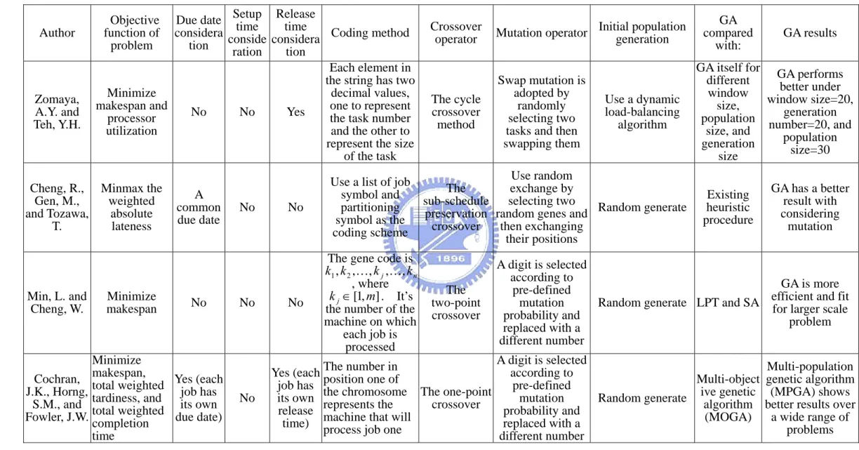
(26) machine scheduling problems with the objective of minimizing total flow time and earliness/tardiness penalties. They proposed a genetic algorithm combined with a simplex method to generate an effective set of Pareto-optimal schedules. Vignier et al. [31] provided a hybrid method to solve a parallel-machine scheduling problem with minimizing the total cost of assignment and setup time and the result showed efficient in industrial case.. Lin [32] considered a unrelated parallel machine. scheduling problem with due date restriction for minimizing makespan, total weighted tardiness, and total weighted flow time.. She proposed a genetic algorithm combined. with prescribed initialization for solving the multi-objective and the result expressed that the GA with prescribed initialization could find an optimal solution in small sized problems. Table 1 shows the differences of GA these researchers developed.. 17.

(27) Table 1. The comparison of GA under various problem characters, crossover, and mutation.. Author. Zomaya, A.Y. and Teh, Y.H.. Release Due date Setup time time Coding method considera conside considera tion tion ration Each element in the string has two decimal values, Minimize one to represent makespan and No No Yes the task number processor and the other to utilization represent the size of the task Objective function of problem. Cheng, R., Minmax the weighted Gen, M., absolute and Tozawa, lateness T.. Min, L. and Cheng, W.. Minimize makespan. A common due date. No. Minimize (each Cochran, makespan, weighted Yes job has J.K., Horng, total and its own S.M., and tardiness, weighted due date) Fowler, J.W. total completion time. No. No. No. No. Use a list of job symbol and partitioning symbol as the coding scheme. No. The gene code is k1 , k 2 ,K, k j ,K, k n , where k j ∈ [1, m] . It’s the number of the machine on which each job is processed. Crossover operator. population Mutation operator Initial generation. The cycle crossover method. Swap mutation is adopted by randomly selecting two tasks and then swapping them. Use a dynamic load-balancing algorithm. Use random exchange by The selecting two sub-schedule preservation random genes and Random generate then exchanging crossover their positions. The two-point crossover. GA compared with:. GA results. GA itself for GA performs different better under window window size=20, size, generation population number=20, and size, and population generation size=30 size Existing heuristic procedure. GA has a better result with considering mutation. A digit is selected according to GA is more pre-defined efficient fit Random generate LPT and SA for largerand mutation scale probability and problem replaced with a different number. A digit is selected Multi-population number in according to Yes (each The genetic algorithm Multi-object position one of pre-defined job has the chromosome The one-point (MPGA) shows ive genetic Random generate algorithm mutation its own represents the crossover better results over probability and release machine that will (MOGA) a wide range of replaced with a time) process job one problems different number. 18.

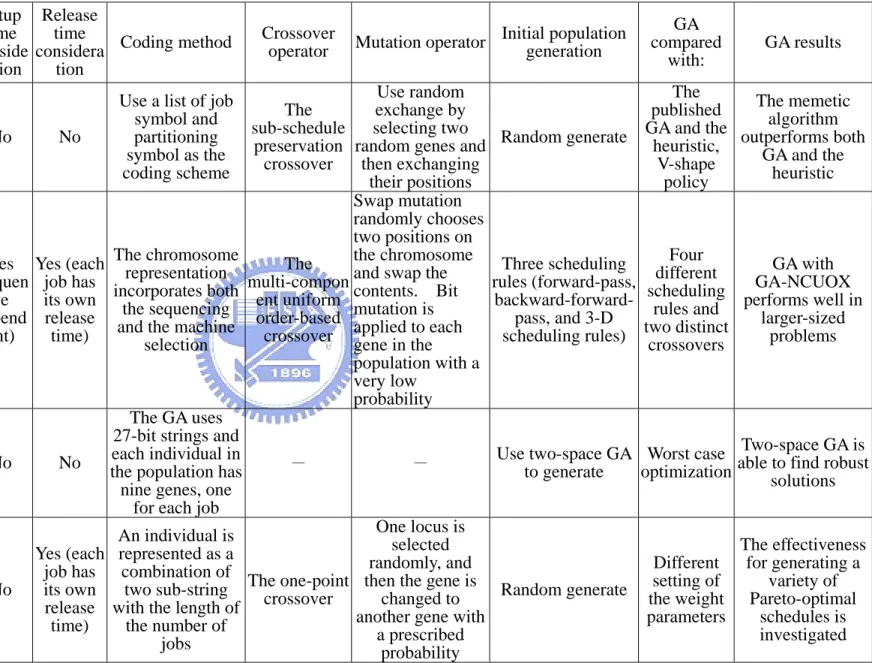
(28) Table 1. Continued. Author. Objective function of problem. Release Due date Setup time time Coding method considera conside considera tion tion ration. Minimize the A maximum Cheng, R. common weighted and Gen, M. due date absolute lateness. total Serifoglu, Minimize weighted F.S. and and Ulusoy, G. earliness tardiness. Herrmann, J.W.. Minimize makespan. Minimize total Tamaki, H., flow time, total weighted Nishino, E., and Abe, S. earliness and tardiness. No. No. Yes Yes (each Yes (each (sequen job has job has its own ce its own depend release due date) ent) time). No. Yes (each job has its own due date). No. No. No. Yes (each job has its own release time). Use a list of job symbol and partitioning symbol as the coding scheme. The chromosome representation incorporates both the sequencing and the machine selection. Crossover operator. population Mutation operator Initial generation. Use random exchange by The selecting two sub-schedule preservation random genes and then exchanging crossover their positions Swap mutation randomly chooses two positions on the chromosome The swap the multi-compon and contents. ent uniform mutation is Bit order-based applied to each crossover gene in the population with a very low probability. The GA uses 27-bit strings and each individual in the population has nine genes, one for each job. －. －. GA results. Random generate. The The memetic published algorithm GA and the outperforms both heuristic, GA and the V-shape heuristic policy. Three scheduling rules (forward-pass, backward-forwardpass, and 3-D scheduling rules). Four GA with different GA-NCUOX scheduling performs well in rules and larger-sized two distinct problems crossovers. Two-space GA is Use two-space GA Worst case able to find robust to generate optimization solutions. One locus is An individual is selected represented as a randomly, and combination of The one-point then the gene is Random generate two sub-string changed to crossover with the length of another gene with the number of a prescribed jobs probability 19. GA compared with:. Different setting of the weight parameters. The effectiveness for generating a variety of Pareto-optimal schedules is investigated.

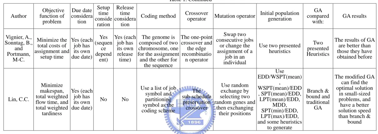
(29) Table 1. Continued Author. Objective function of problem. Release Due date Setup time time Coding method considera conside considera tion tion ration. Crossover operator. population Mutation operator Initial generation. Swap two Vignier, A., Minimize the Yes (each Yes Yes (each The genome is The one-point consecutive jobs Sonntag, B., total costs of job has (sequen job has composed of two crossover and or change the Use two presented the edge its own chromosome, one ce and heuristics assignment of a its own assignment and depend release for the assignment recombinatio Portmann, job in an due date) setup time and the other for n operator time) ent) M-C. individual the sequence Use EDD/WSPT(mean) , Use random Minimize WSPT(mean)/EDD Use a list of job exchange by The makespan, Yes (each , SPT(mean)/EDD, symbol and selecting two sub-schedule job has total weighted No No partitioning Lin, C.C. flow time, and its own preservation random genes and LPT(mean)/EDD, MDD, symbol as the then exchanging SPT(min)/EDD, crossover total weighted due date) coding scheme their positions tardiness LPT(max)/EDD, and some heuristics to generate. 20. GA compared with:. GA results. The results of GA Two are better than presented those they have Heuristics obtained before. The modified GA can find the optimal solution Branch & in small-sized bound and problems, and traditional have a better GA solution speed than branch & bound.

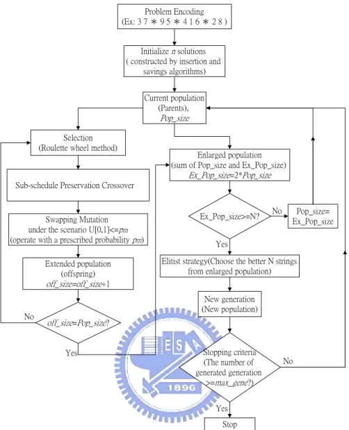
(30) 4.2 The Hybrid Genetic Algorithm. GA is an artificial adaptive system for simulating natural evolution. Because of their effectiveness and efficiency in searching complex spaces, they are increasingly used to attack NP-hard problems. The core of GA is its crossover operator that progressively constructs near optimal solutions from good feasible solutions. In this paper, we propose a new crossover that protects better schedules of machines from elimination.. First of all, we would give some definition of terms including. Pop _ size ,. Ex _ Pop _ size , max_gene, off_size, and. pm .. Let notations. Pop _ size and Ex _ Pop _ size be the number of parents and extended population individually, off_size be the number of offspring, and max_gene be the maximum number of generated generation. Besides, let p m be the prescribed probability of mutation. The flowchart of the execution for hybrid genetic algorithm is given in Fig. 2.. 21.

(31) Problem Encoding (Ex: 3 7 ＊ 9 5 ＊ 4 1 6 ＊ 2 8 ) Initialize n solutions ( constructed by insertion and savings algorithms) Current population (Parents),. Pop_size Selection (Roulette wheel method). Enlarged population (sum of Pop_size and Ex_Pop_size) Ex_Pop_size=2*Pop_size. Sub-schedule Preservation Crossover No. Pop_size= Ex_Pop_size. Swapping Mutation under the scenario U[0,1]<=pm (operate with a prescribed probability pm). Ex_Pop_size>=N?. Extended population (offspring) off_size=off_size+1. Elitist strategy(Choose the better N strings from enlarged population). No. Yes. New generation (New population). off_size=Pop_size? Stopping criteria (The number of generated generation >=max_gene?). Yes. No. Yes. Stop. Figure 2. The flowchart of the execution for hybrid genetic algorithm. 4.2.1 Problem encoding. Normal binary encoding does not work very well for the parallel-machine scheduling problem because the encoding strings may become too redundant to incorporate all needed messages.. Therefore, we code the strings by using the. representation of decimal numbers.. We use a set of integers and stars ＊. representing the job identity and the partition of jobs to machines for parallel-machine scheduling problem.. The integers and stars on the string represent all possible. sequences of jobs on parallel machines. For a problem of n jobs and m parallel machines, a correct chromosome must consist of n job symbols and m-1 partitioning symbols ＊, which mean there should be n+m-1 genes in a chromosome.. 22. We can.

(32) give a simple example of 9 jobs and 4 parallel machines shown below. The string can be represented as follows: [37 ＊ 95 ＊ 416 ＊ 28] 4.2.2 Initialization. In each generation the GA manipulates a set of operators in the population. The construction of the initial population is important since the operators of GA would preserve some part of better chromosomes generation to generation.. The initial. population influences not only the convergence of the GA but the qualities of chromosomes generated.. The initial chromosomes are constructed with network. algorithms we described in this identical parallel-machine scheduling problem.. We. are looking for the better near optimal solution produced by the initial population based on network algorithms than a randomly generated population. We also predict the quick convergence of the GA with the constructed initial population. 4.2.3 Selection. During each generation, we can use some measure of functions to evaluate the values of chromosomes.. Fitness is estimated based on the objective function in most. cases of optimization problems. As the objective of our problem is WPSP with minimizing makespan, we can use the reciprocal of the objective function as the fitness value. So a fitter chromosome has a larger fitness value. The fitness value of each chromosome is defined as following: ⎡ K − k + 1⎤ F (α , β ) = (Cmaxα , β ) −1 × ⎢ ⎥ ⎢ K ×Q ⎥. (37). where the term C maxα ,β expresses the makespan of the α th chromosome in the pool when the GA cycle proceeds to the β th generation. The term K represents the available machine number and k represents the actual required machine number. Besides, the term Q is a constant described in section 2 for keeping the calculation ( K − k − 1) / KQ moving around 0 and 1. So the function ⎡K − k / KQ ⎤ can make sure that the fitness value calculated by equation (37) is available to be used. 23.

(33) The selection technique in this paper is based on the roulette wheel method. In this case, the probabilities of the individual chromosomes surviving to the next generation determine the slots of the roulette wheel. These probabilities of these slots on the roulette wheel are estimated by dividing the fitness value of each chromosome by the sum of the fitness values of all chromosomes in the current population. Cumulating the probabilities of each chromosome creates the individual slots. Here comes an example, which calculates the individual slots on the roulette wheel. There are three chromosomes in the population, of which the probabilities of chromosomes are 0.2, 0.3, and 0.5 individually. Then the slots of chromosome 1, chromosome 2 and chromosome 3 will range from 0-0.2, 0.2-0.5, and 0.5-1 respectively. Each slot size of chromosome will be proportional to its fitness value. 4.2.4 Genetic operators. Two genetic operators, crossover and mutation, are usually used in the genetic algorithm.. Crossover generates offspring by combining two chromosomes’ features.. Mutation operates one chromosome by randomly selecting two genes and swapping them. Generally specking, the crossover operator plays an important role for the performance in the GA cycle. The performance of crossover in each operator does affect the performance of GA. crossover and mutation.. So we adopt the different rules for designing. Both crossover and mutation can handle the job. permutation and setup time on the identical parallel machines, so the methods of crossover and mutation should be suitable for use. Crossover Because the WPSP with minimum makespan has the job due date problem, the chromosome may have a bad fitness value, an infeasible solution, through the traditional crossover operator. We provide a new crossover considering the time postponement concept to figure out the problem with due date restriction. The time postponement is the value that the non-expected event can delay for at most.. The. crossover operates two parents and creates a single offspring. It breeds the primary partitioning structure and better sub-schedules into offspring from one parent and then 24.

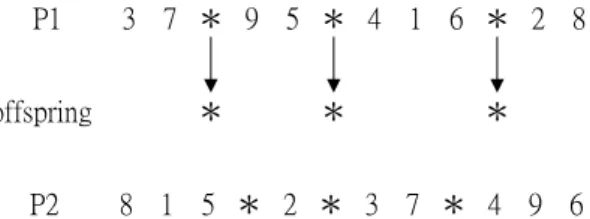
(34) fills the offspring with remaining genes derived from the other parent. The selection of sub-schedule is considering the job slackness, the time postponement, on each identical parallel machine. The crossover copies the better sub-schedules on some identical parallel machines from one parent to the offspring for preserving the good permutation of jobs. The other empty positions of the offspring can be filled with one way, which is a left-to-right scan from the other parent. We let Cνk be the completion time of job, dνk be the due date of job on ν th position of machine mk , n be the number of job consideration on machine mk , and N k be the number of jobs on machine mk . Equation (38) indicates the slackness of job on ν th position of machine mk .. SSLνnk of equation (39) means the sum of slackness values for n. consecutive jobs on machine mk , which are located from ν th to (ν + n − 1) th position. After calculating the value SSLνnk , we can estimate the average value of slackness SSLνnk for n jobs started from ν th to (ν + n − 1) th position on machine mk . The estimations of slackness values are defined as following: SLνk = dνk − Cνk , ν = 1,2,K, N k ; k = 1,2,K, K. (38). ν + n −1. SSLνnk = ∑ SLνk , ν = 1,2,K, N k ; 1 ≤ n ≤ N k −ν + 1 ; k = 1,2,K, K. (39). SSLνnk = SSLνnk × n −1. (40). ν. In the beginning of crossover, GA would choose one parent with better fitness value and breed the partitioning structure of the parent into the offspring as shown in Figure 3. P1 offspring P2. 3 7 ＊ 9 5 ＊ 4 1 6 ＊ 2 8 ＊. ＊. ＊. 8 1 5 ＊ 2 ＊ 3 7 ＊ 4 9 6. Figure 3. Copy the partitioning structure to offspring Then for all jobs on each machine, GA calculates SSLνnk of all combinations of jobs in sequences and derives each SSLνnk from each SSLνnk . Choose the smallest SSLνnk for each machine and put the job combinations into the sub-schedules as 25.

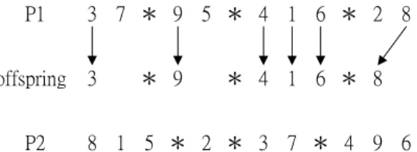
(35) shown in Figure 4. P1. 3 7 ＊ 9 5 ＊ 4 1 6 ＊ 2 8. offspring P2. 3. ＊ 9. ＊ 4 1 6 ＊ 8. 8 1 5 ＊ 2 ＊ 3 7 ＊ 4 9 6. Figure 4. Copy the sub-schedules to offspring from the parent with better fitness value. Finally, GA would use a left-to-right scan to fill the offspring with remaining genes derived from the other parent as shown in Figure 5. Starting point on offspring. P1. 3 7 ＊ 9 5 ＊ 4 1 6 ＊ 2 8. offspring. 3 5 ＊ 9 2 ＊ 4 1 6 ＊ 8 2. P2. 8 1 5 ＊ 2 ＊ 3 7 ＊ 4 9 6. Figure 5. Fill the empty of the offspring from the other parent. After recounting the execution of crossover, here is the procedure of crossover divided into three steps. Step1. Get the partitioning symbol ＊ from one parent which has better fitness value. Step2. Choose the sub-schedules from the parent with better fitness value. Let parameters k and ν be one. The selection of sub-schedules is as following: Step 2-1. For the ν th position of machine mk on the chromosome, calculate the slackness value SLνk of job ri on ν th position. Step 2-2. Let ν = ν + 1 . If the value ν is larger than N k , go to step2-3. Otherwise, calculate the slackness value SLνk of job on the ν th position of machine mk and go to step2-1. Step 2-3. For ν = 1,2,K, N k and 1 ≤ n ≤ N k −ν + 1 , estimate all kinds of average slackness value SSLνnk . Select the largest one SSL ν ′n′k among all SSLνnk and put the job combination from ν ′ th position to ν ′ + n′ − 1 th position on machine into the sub-schedule of machine mk . Step 2-3. Let k = k + 1 and check the constraint of the number of available machines K. If k is larger than the number of available machines K, then go to step 2-4. Otherwise, Let index ν be one and go to step2-1. 26.

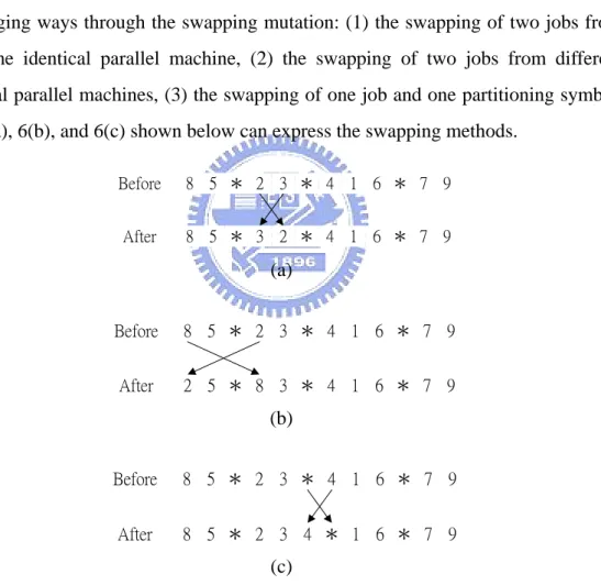
(36) Step 2-4. Select the K sub-schedules of all machines and copy the K sub-schedules to offspring. Step 3. Fill the empty of the offspring with the unscheduled genes by making a left-to-right scan from the other parent without violating the job due date restriction. The starting point of the filling can be generated randomly. Mutation We use the swapping technique as the mutation method in this paper.. The. mutation proceeds by randomly choosing two genes on the chromosome and then swapping them. If the schedule shows infeasible after mutation technique, we would preserve the original one from due date violence.. There are three possible. exchanging ways through the swapping mutation: (1) the swapping of two jobs from the same identical parallel machine, (2) the swapping of two jobs from different identical parallel machines, (3) the swapping of one job and one partitioning symbol. Fig. 6(a), 6(b), and 6(c) shown below can express the swapping methods. Before. 8 5 ＊ 2 3 ＊ 4 1 6 ＊ 7 9. After. 8 5 ＊ 3 2 ＊ 4 1 6 ＊ 7 9. (a) Before. 8 5 ＊ 2 3 ＊ 4 1 6 ＊ 7 9. After. 2 5 ＊ 8 3 ＊ 4 1 6 ＊ 7 9. (b) Before. 8 5 ＊ 2 3 ＊ 4 1 6 ＊ 7 9. After. 8 5 ＊ 2 3 4 ＊ 1 6 ＊ 7 9. (c) Figure 6. Illustration of swapping technique 4.2.5 Elitist Strategy. When the number of offspring in the pool is reaching to the expected level, we will mix the offspring with the original parents to get the enlarged population. Then we. 27.

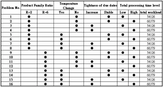
(37) use the roulette wheel as the concept of elitist strategy for choosing the better part of the enlarged population.. That means the fitter chromosome is selected first for. surviving to the next generation. In our GA cycle, the elitist way is to preserve the better chromosomes in each generation and reduce the errors of stochastic sampling. Through the elitist strategy, the number of chromosomes in each generation will be equal to the original population we determined in the beginning. 4.2.6 Stopping Criteria. After the genetic operators and elitist strategy, the fitness of each chromosome in the population will be re-estimated by using the fitness function. There are several rules to decide if the GA cycle should be stopped: (1) see if the chromosomes in the current population are fitter than the ones in the previous population by calculating the total and average fitness values of all chromosomes in every cycle, (2) see if the best chromosome in the current GA pool is fitter than the best one in the old GA pool by calculating the fitness value of the best chromosome in every cycle, (3) see if the number of generation reaches to the level we requested. We choose the item (3) according to the convenience of GA operation. Therefore, in our experiment, the GA operation will be terminated if the number of generation reaches to what we prescribed.. 5. Problem Design and Testing For the sake of comparing the performance of improving heuristics and the hybrid genetic algorithm, we design a set of 16 problems with different circumstances for testing. Each problem includes 25 parallel identical machines and 100 jobs, which are divided into 30 product types and should be completed before the given due date. The 100 jobs would be processed on the 25 parallel identical machines and each machine capacity is set to be three days, 4320 minutes. Here “minute” is used as the time unit for job processing time, job due dates, setup time, and machine capacity. In this paper, we highlight the impact of setup time of consecutive jobs from different product families or different operation temperatures. So the time cost by changing. 28.

(38) probe card before the machine is ready to process the coming job with different product family is set to 80 or 120 minutes (80 or 120 minutes is according to different product family). The required times of adjusting temperature from room to high is set to be 60 minutes, from high to room is set to be 80 minutes, and from high to high is set to be 140 minutes. Because the time of adjusting temperature from room to room does not need to warm up or cool down the machine, it is set to be 0 minutes. The time of loading code before the machine is ready to process the coming job with different product type is set to be 5 minutes. And the initial setup time of machine from idle to processing state is set to be 100 minutes. The setup time of consecutive jobs from same product type is set to be 0 minutes under all operation temperatures. The problem design is based on the wafer probing shop floor in an IC manufacturing factory of the Science-based Industrial Park, Taiwan. The problem test is divided into four factors, which contains (1) the product family ratio, including two grouping levels R2 and R6, (2) the tightness of due dates, including stable and increasing states, (3) the consideration of adjusting temperature, including setup time with temperature consideration or not, (4) the total processing time, including low and high levels. Product Family Ratio (R) The distribution of jobs to the product families is related to the setup time of consecutive jobs. We need to evaluate the influence of product families on the performance of scheduling solutions via the factor, product family ratio. If a product family has large number of jobs, it may lead to a smaller value of total setup time of scheduling solutions. Oppositely, if a product family has small number of jobs, it may result in a larger value of total setup time of machine schedules. Here we define an index, product family ratio, which is the division of the number of job product types by the number of job product families. There are 100 jobs divided into 30 product types in our test problem. For example, if the value of product family ratio is 2, it means that 30 product types of 100 jobs are distributed into 15 product families randomly. In our design, there are two levels for testing, R2 and R6, which means. 29.