貨幣政策對房屋市場的影響之探討 —動態隨機一般均衡模型分析 - 政大學術集成

全文

(1)國立政治大學經濟學系碩士論文 Department of Economics College of Social Science National Chengchi University Master Thesis. 學. ‧ 國. 立. 政治大. 貨幣政策對房屋市場的影響之探討. Nat. sit. y. ‧. —動態隨機一般均衡模型分析. n. er. io. The Effect of Monetary Policy on Housing Market—A Dynamic Stochastic a General Equilibrium Framework v. i l C n U hengchi 曾楷仁 Tzeng, Kai-Ren. 指導教授：黃俞寧博士 Advisor: Hwang, Yu-Ning, PhD 中華民國 103 年 5 月.

(2) 謝辭時間過得很快，轉眼間也走到了研究所生活的尾聲；看著這一本碩士論文從一個又一個的模型推導檔案和程式碼，到一篇完整的論文，心中有許多複雜的感動。謝謝我的論文指導老師黃俞寧老師這兩年碩士班路程在論文上及在學習過程中的照顧，感謝老師的細心教導，帶著我了解模型、程式以及寫學術論文的格式要求，也教導了我很多人生的道理，老師對我的付出和包容，我會永遠記得。感謝口試委員陳南光老師和毛維凌老師在口試當天以學術論文的規格給了我很多的建議和指導，讓我更了解學術論文要注意的重點，也謝謝毛老師這兩年來在課堂上及課堂外的教導。這兩年的碩班生活，要感謝很多人的照顧和鼓勵。謝謝系主任陳心蘋老師這兩年的照顧，謝謝老師給我嘗試擔任經濟學助教的機會，從一開始的懵懂到之後的熟練，老師總是耐心地帶著我，和老師合作的過程，常常可以感受到老師對學生的關心和信任。謝謝劉世夫學長在論文上提供我很多協助，謝謝學長在程式上的教導和幫我偵錯；謝謝老師的助理馥菁學姐在口試還有論文的幫忙。謝謝政大經研 102 級的夥伴們，感謝同為俞寧老師指導的搭檔夥伴仁川，陪我一起走過托. 立. 政治大. ‧. ‧ 國. 學. 福考試和論文，我很喜歡我們一起努力、一起聊天的日子。謝謝柏祐、家毅、彥儒、安易和顯貴這兩年的陪伴，謝謝你們的包容和照顧，從碩一我們一起在總圖 B1 準備考試，和每一次一起出遊聚會，我都會記得，因為有你們這兩年的碩班生活更精采。謝謝國際英文演講社的每個夥伴，謝謝我的好兄弟建幟從大四下學期到今天一路的力挺和在社團事務的扶持協助，在社團我們一起完成了很多事，而在很多. sit. y. Nat. n. al. er. io. 生活和關於未來的問題，也謝謝你給了我很多想法，也謝謝你在我論文遇到最大考驗的時候，在社團值班室陪伴著我一起度過難關和鼓勵；我很幸運可以在這一個大家庭裡和你們一起學習、一起成長。還有要謝謝很多這兩年來很多幫助過我的貴人，謝謝河山學舍讓我從大一到碩一能有一個像家一樣溫暖的宿舍，和你們吃飯聚會的夜晚也讓我開拓了很多視野。. Ch. engchi. i Un. v. 最後，我要感謝我的家人從小到現在一路來的支持和照顧，謝謝父母一路來的栽培，讓我能順利完成碩士，以及在論文的修改也給了我很多的建議。謝謝一路來幫助過我和支持鼓勵我的每個人，雖然無法在這邊一一列出，但是我會永遠銘記在心；未來的人生，我會利用碩班累積的力量和養分，更勇敢地更努力地闖出一片屬於自己的天空! 曾楷仁謹誌於政大經濟系民國 103 年 6 月.

(3) 中文摘要本文的研究目的是在動態隨機一般均衡模型的架構中，比較不同貨幣政策之下，外生衝擊對房價及總體變數的衝擊反應；本文建立一個封閉經濟體系，其中包含家計單位、房屋擁有者、房屋建商及商品生產部門，並且由一個貨幣當局制訂利率政策；本文探討三種利率法則:傳統的泰勒法則、加入房價目標的利率法則、通貨膨脹目標的利率法則及一個激進的通貨膨脹目標利率法則，我們分別在這四種利率政策下模擬成本衝擊、技術衝擊、貨幣衝擊及家計單位對房屋的偏好衝擊，比較這三種政策下房價和其他變數的衝擊反應函數；本文發現加入房價目. 政治大. 標對房價穩定沒有顯著的影響，而傳統的泰勒法則相對於通貨膨脹目標的利率政. 立. 策對房價穩定比較有幫助. ‧. ‧ 國. 學. n. er. io. sit. y. Nat. al. Ch. engchi. i Un. v. 關鍵字: 動態隨機一般均衡模型、房價、貨幣政策、泰勒法則、房價目標、通膨目標.

(4) Abstract The main purpose of this paper is to compare the effect of various shocks on house price and other macroeconomic variables under different monetary policies using micro-based dynamic stochastic general equilibrium (DSGE) analysis. We construct a closed economy with a representative household, a representative house owner, a house producer, a producer of goods and a monetary authority that implements monetary policies. We discuss three interest rate policy settings, which include traditional Taylor’s Rule, Taylor’s Rule with house price targeting and an. 政治大. inflationary targeting monetary policy followed by an aggressive inflationary. 立. targeting rule. We compare the impulse response function with an inflationary shock,. ‧ 國. 學. a technology shock, a monetary shock and a household’s preference shock under these monetary policies. We discover that adding house price targeting into traditional. ‧. Taylor’s Rule does not work better in house price stabilization. Our results show the. y. Nat. n. al. er. io. sit. apparent importance of Taylor’s rule in house price stabilization.. Keywords:. Ch. i Un. v. house price, monetary policies, Taylor’s rule, house price targeting,. engchi. inflationary targeting , dynamic stochastic general equilibrium.

(5) Contents 1. Introduction...............................................................................................................1 1.1. Motivation…………………………………………………………………..1. 1.2. Literature Review……………………………………………………………4. 2. The Model……………………………………………………………………….....8 2.1. Household…………………………………………………………………..8. 2.2. House owner………………………………………………………………..9. 2.3. The House Producer………………………………………………………..11. 2.4. Good Firm………………………………………………………………….12. 2.5. Monetary Policies………………………………………………………….13. 2.6. Exogenous Variables…………………………………………………….....13. 2.7. Market Clearing and Equilibrium……………………………………….....14. 3.1. Parameters Setting………………………………………………………....15. 3.2. Calibration Results………………………………………………………....17. 政治大 3. Calibration…………………………………………………………………………15 立. ‧ 國. 學. Calibration under Taylor’s Rule……………………………………….17. 3.2.2. Calibration under Taylor’s Rule with House Price Targeting………....18. ‧. 3.2.1. sit. y. Nat. 3.2.3 Calibration under Interest Rate Rule with Inflation Targeting………...21 4. Conclusion………………………………………………………………………....28. io. n. al. er. Reference……………………………………………………………………………..29. i Un. v. Appendix……………………………………………………………………………..31. Ch. engchi.

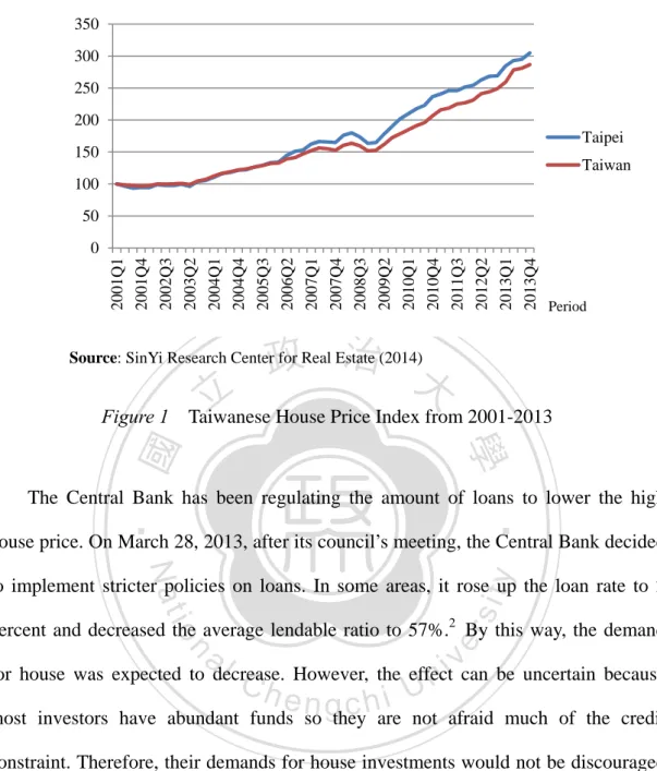
(6) 1. Introduction 1.1 Motivation High house price has been the top on the list of Taiwanese “top ten complaints”. It becomes an over burden for many Taiwanese to buy a house on their own. The house price to income ratio has been growing sharply especially in Taipei. It increased from 6.4 in June, 2003 to 15 in December, 2013. The house price to income ratio for the five major cities of Taiwan jumped from 5.26 in June, 2003 to 8.3 in December, 20121. The burden of high house price has led to other social problems such as lower. 治政 birth rate. This issue has been studied in Chang, Chen, 大Teng and Yang (2009). They 立 found that there is a large bubble in Taipei’s house market, which indicates that, ‧ 國. 學. Taipei’s house price in that period is far above the reasonable level.. ‧. Taiwanese house price has grown significantly in the past ten years. According to. sit. y. Nat. the data from Sin-yi Research Center for Real Estate, the house price in Taipei and the. io. al. er. overall average house price in Taiwan started to grow rapidly in 2003. Though there was a decrease in house price in response to the crisis during the period of Financial. n. iv n C Crisis of 2007 to 2008, the house price again in the second quarter of 2009. h e nboomed gchi U. After 2009, there has been a continuous positive growth in the house price. By the end of 2013, the house price index has become 3 times as the one in 2001. Despite the fact that there have been some fiscal policies implemented, there house price did not drop significantly in response to the policies..                                                         Taiwanese Economic Journal (2014), Taiwanese House Price to Income Ratio (Database), Retrieved from Taiwanese Economic Journal Database. 1 1.

(7) 350 300 250 200 Taipei 150. Taiwan. 100 50 2001Q1 2001Q4 2002Q3 2003Q2 2004Q1 2004Q4 2005Q3 2006Q2 2007Q1 2007Q4 2008Q3 2009Q2 2010Q1 2010Q4 2011Q3 2012Q2 2013Q1 2013Q4. 0. Period. 政治大. Source: SinYi Research Center for Real Estate (2014). 立. Taiwanese House Price Index from 2001-2013. 學. ‧ 國. Figure 1. The Central Bank has been regulating the amount of loans to lower the high. ‧. house price. On March 28, 2013, after its council’s meeting, the Central Bank decided. y. Nat. sit. to implement stricter policies on loans. In some areas, it rose up the loan rate to 2. n. al. er. io. percent and decreased the average lendable ratio to 57%.2 By this way, the demand. Ch. i Un. v. for house was expected to decrease. However, the effect can be uncertain because. engchi. most investors have abundant funds so they are not afraid much of the credit constraint. Therefore, their demands for house investments would not be discouraged too much. There have been some literatures discussing the housing price problem in Taiwan. Some papers such as Chang, Chen, Teng and Yang (2009) estimated the growing house price bubbles in Taipei. Chen and Cheng (2012) discussed the effect of financial accelerator on housing market and the relationship of external finance                                                         2. Central Bank of China (Taiwan) (2013), Meeting of Board of Central Bank Committee (News Announcement No 130), Retrieved from http://www.cbc.gov.tw/ct.asp?xItem=44416&ctNode=302& mp=1. 2 . .

(8) premium and other macroeconomic variables. However, not too many efforts have been devoted to discussions about the effect of interest rate policy on housing market in Taiwan using the traditional Dynamic Stochastic General Equilibrium model setting. The asset price has been discussed in the literatures such as Bernanke, Gentler and Gilchrist (1999), in which the effect of external finance premium on macro variables was discussed. In order to prevent the default risk, collateral constraint and nominal debt contract were added, as in Iacoviello (2005). An interest rate policy that follows Taylor’s rule has been implemented in. 治政 Taiwan. According to Lin (2012), the interest rate with大 Taylor’s rule functions well in 立 stabilizing price level and encouraging economic growth. However, this setting could ‧ 國. 學. not help in stabilizing house price. He suggested that some variables related to. ‧. housing market should be added, such as housing demand or house price index. The. sit. y. Nat. monetary policy has been criticized for that the interest rate is not adjusted when the. io. er. house price grows. While the house price is rising, the interest rate in Taiwan is still. al. n. low so that the cost of house investment remains low. It could not respond to the. i n house price growth or the houseC demand. U hengchi. v. The purpose of this paper is to calibrate the effect of different interest rate rules on house price. We would like to examine whether an interest rule taking house price growth into account will lower the growth of house price with DSGE model. Also, we would like to verify the importance of Taylor’s Rule interest rate setting in stabilizing the house price. We follow the model in Aoki (2002) and we use the setting of Chen and Cheng (2012) with some modification in the household sector. We examine the effects of different monetary policies on macroeconomic variables under different shocks. The rest of the paper is organized as follows. In Section 1.2, we review the 3 .

(9) related literature. The model will be described in Section 2, with first order condition and monetary policy. In Section 3, we show the results of calibration and compare the results of different monetary policies. Finally in Section 4, we make the conclusion according to our calibration and point out some issues for future research. 1.2 Literature Review Let us review a little bit on literatures related to this work.. We start with. literature on capital investment with external finance premium using DSGE model, and then, move on to those with housing market and borrowing constraint. Lastly, we. 治政 will look at literatures about effect of monetary policies 大on asset pricing and how it is 立 associated with Taiwanese housing market. ‧ 國. 學. Before we look at how monetary policies or related financial conditions affect. ‧. the housing market, we shall have a look on how financial properties such as financial. sit. y. Nat. accelerator and credit market imperfection influence investment and the price of. io. er. capital. A classical literature for this issue is Bernanke, Gertler and Gilchrist (1999),. al. which set up a DSGE model with entrepreneur who invests capital for production. n. iv n C input and seeking capital gain. Thehentrepreneur borrows e n g c h i U fund from a financial sector, which bear the risk that the debt could not be realized. Therefore, the financial sector decides its loan rate according to the default risk. The entrepreneur chooses its optimal capital investment based on the price of capital, loan rate given by the financial sector and the depreciation rate. Furthermore, a government sector decides the fiscal and monetary policy. Bernanke, Gertler and Gilchrist (1999) discusses the effect of exogenous shock on macroeconomic variables with and without financial accelerator. Output and investment change more with financial accelerator when there is an exogenous shock. In the cases with investment delays, financial accelerator will exacerbate the exogenous effect on investment and output as well. 4 .

(10) Next, we take a look at some literatures that discuss the housing market with a DSGE model. In Chen and Cheng (2012), the authors suggest that there are two types of households, a representative house-owner and a consumer who rents houses from the house-owner. Consumer can spare his income in consumption, house-renting or money-holding. For the individual house-owner, he borrows funds from financial sectors for house-investing. Chen and Cheng (2012) assumes the existence of default risk on the individual house-owner. According the risk, the financial sector sets its house loan rate which is higher than the saving rate. This difference is the external financial premium. In the production sector, Chen and Chang (2012) sets a house. 治政 production firm with linear production technology, an 大intermediate-good firm with 立 house and labor as input, and a retailer that uses Calvo pricing. Lastly, there is a ‧ 國. 學. central bank which implements its monetary policy according to Taylor’s rule. Chen. ‧. and Chang (2012) discusses the relation of fluctuations of external financial premium. sit. y. Nat. and macroeconomic variables in response to various shocks. From the calibration in. io. er. Chen and Chang (2012), the effect of exogenous shocks on external premium and. al. house price turn out to be in opposite ways. For instance, a decrease in wealth would. n. iv n C increase the external financial premium because the default risk of house-owners heng chi U increases while the house price decrease owing to a negative income effect on demand. for houses. Chen and Chang (2012) concludes that a decrease in house price caused by exogenous shocks will increase the default risk owing to a decrease in return, therefore push the external financial premium to increase. The rise in external financial risk premium will increase the investment cost for houses, therefore discourage the housing investment and lowers the house price. Furthermore, the financial accelerator will strengthen the effect of exogenous shocks. Similar discussion about financial accelerator in housing market can also be found in Aoki (2002), in which there are two types of consumers, representative house 5 .

(11) owner, house producer and final goods producer. The major difference is that the consumer who follows permanent income hypothesis decides its consumption in period t and certain ratio of consumption will goes to house renting, while the rest will be consumption on other goods. Also, houses are only bought by the representative house owner and are not used in production. In addition to the effect of financial accelerator, Aoki (2002) also discuss the effect of the elasticity of transfer with respect to leverage ratio on macroeconomic variables. Higher elasticity of transfer will decrease the growth in house price and house investment in response to interest rate shock but the effect on consumption will be larger.. 治政 Iacoviello (2005) uses the housing market to discuss 大 the effect of collateral 立 constraint to the macroeconomic variables with nominal debt contracts and collateral ‧ 國. 學. constraints. In Iacoviello (2005)’s model, there are patient and impatient households. ‧. along with entrepreneurs and policy maker. The entrepreneurs use houses as. sit. y. Nat. production input and households gain utility from buying houses. From the calibration,. io. er. a positive house-price shock without collateral effect will lower the consumption and. al. when the collateral effect increases, the effect for consumption will become positive.. n. iv n C In the later part, Iacoviello (2005) discusses central banks should response to h e n gwhether chi U. housing price by examining the effect of change of correlation between asset price and interest rate. A small increase of the correlation between interest rate and house price does not change the fluctuation of output and inflation rate. This suggests that a monetary policy responding to housing price does little on stabilizing the economy. Next, we will look at some literatures discussing the effect of monetary policy on asset price. Bernanke and Gertler (1999) discusses the effect of monetary policies on macroeconomic variables with asset bubble shock and inflation shock. The authors follow most of the setting in their paper of 1999. They compare the impulse response on interest rate in response to expected interest rate, current interest rate and interest 6 .

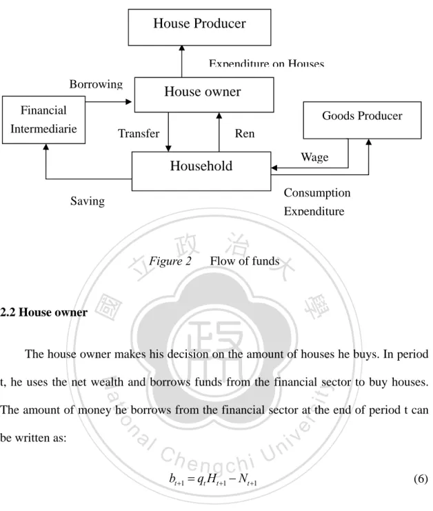
(12) rate in respond to the market price of assets as well as inflation rate. Also, they compared the effect of different parameter settings. Their major conclusion is that a monetary policy that responds to asset price is not necessary or desirable for price stabilizing. Also, an aggressive interest rate rule with inflation gap will decrease the variability of asset price and output gap. Central Bank of China (Taiwan) points out that low interest rates do not necessarily lead to higher house price in a report published in February, 2014. CBC (2014) uses some empirical facts from IMF to show that many countries such as British has a high interest rate but the growth rate in house price is larger than United. 治政 State, which implements a lower interest rate. Also 大 from some empirical facts, the 立 effect of interest rates on house price is not significant. Therefore, increasing interest ‧ 國. 學. rate is not an effective policy on lowering the house price. The CBC claims other. er. io. sit. y. Nat. 2. Model. ‧. non-interest rate policies such as lowering funds lending rate is more desirable.. al. n. iv n C We consider a closed economy representative household, house-owner, h with e n the gchi U house producer, good firm and monetary authority. In our model, the representative household rent houses from the representative house-owner. The flow of funds is shown as Figure 2. 2.1 Household without houses The household maximizes his lifetime utility by allocating his income to consumption of goods, house renting from house-owner and money holding. Also, he has to decide the amount of labor supply. His lifetime utility function can be written as follows: 7 .

(13) . E0   t (ln Ct  jt ln H t   ln(1  Lt )) . .. (1). t 0. where Ct denotes the representative household’s consumption in period t, H t denotes the house that the representative household rents from house owner in period t, and jt is the parameter for household’s preference on houses. The budget constraint for household in period t is: dt-1 Ct  xth H t  d t  Rt 1d t 1  wt Lt  Ft h. (2). 政治大. where xth is the house rental price in period t, dt 1 the deposit in period t-1, Ft h. 立. 學. ‧ 國. the lump-sum transfer from house-owner, and Rt 1 the real interest rate. Solving the optimization problem we yield the following:. 1 R   E t ( t ) . . .. . (3) Ct C t 1. Nat. y. ‧.                           . sit. io. n. al. xth j  t . (4) Ct H t. er.                              . Ch. i Un. v. wt (1  Lt )   Ct (5) . engchi. From (3), in steady state we can get the relationship of interest rate and inflation: R. 1. . 8 .

(14)        . House Producer Expenditure on Houses Borrowing Financial Intermediarie. House owner Goods Producer. Transfer. Ren Wage. Household. Consumption Expenditure. Saving. 治政 Figure 2 Flow of funds 大立 ‧ 國. 學. 2.2 House owner. ‧. The house owner makes his decision on the amount of houses he buys. In period. Nat. sit. y. t, he uses the net wealth and borrows funds from the financial sector to buy houses.. al. n. be written as:. er. io. The amount of money he borrows from the financial sector at the end of period t can. Ch. engchi. bt 1  qt Ht 1  Nt 1. i Un. v. (6). where qt denotes the real house price in period t, Ht 1 the amount of houses he buys at the end of period t, and N t 1 the wealth that the individual house owner has at the end of period t. The individual house owner rents the houses to the individual household at period t+1. The return of buying houses includes rent revenue from the representative households and the net gain of house price:. 9 .

(15) Et ( Rth1 )  Et [. xth1  (1   h ) qt 1 ] (7) qt. During the house purchasing in period t, the representative house owner also faces a borrowing cost. For a house owner seeking to maximize his profit in the house purchase, his optimal house purchase decision will be made at where marginal cost for borrowing will equal the expected return he can receive through house borrowing. Therefore, Rth1 also equals the marginal borrowing cost or the interest rate that the house owner faces for his borrowing decision. We follow the setting in Bernanke, Gertler and Gilchrist (1999).That is, there. 治政 exists difference between the marginal cost of borrowing 大 and real interest rate. We 立 ‧ 國. 學. define st as the external finance premium (EFP), which equals the expected ratio of return on buying houses between real interest rate at period t+1. . ‧. st  Et. sit. y. Nat. Rth1 .. (8) Rt 1. n. al. er. io. However, we assume the absence of financial accelerator in this model. In other. i Un. v. words, the external risk premium will not be affected by the ratio between net wealth. Ch. engchi. and expenditure on houses in period t+1.3.     The representative house owner’s earns his income from the revenue of endowment labor, return on house buying. He also has to pay the loans and transfer payment to the household. Therefore, the wealth of representative house owner in period t+1 can be written as: N t 1  Rth qt 1 H t  sRt bt  Ft h (9)                                                         N t 1 3 In Chen and Chang (2012), the external risk premium equals  ( ) , where  '  0 .After the qt H t 1     log-linearization, it can be written as st  ( N t 1  qt  H t 1 ) , where  is the financial accelerator. Here, we discuss an economy where the external finance premium will not change according to the leverage ratio of the house owner. Therefore, we set  to zero. 10 .

(16) For the lump-sum transfer, we set it as a convex function of. N t 1 , it can be written qt H t 1. as: Ft h   (. N t 1 ),  '  0 (10) qt H t 1. 2.3 The House Producer The house producer uses a linear production technology. The investment for house production can be written as. 政治大. H t  I th  (1   h ) H t 1 . (11). 立. ‧ 國. 學. The representative house producer wants to maximize his profit in period t, the profit maximization problem is as following I th ) H t 1 (12) H t 1. sit. y. Nat. n. al. er. I th ) is a convex function that represents the adjustment cost function of H t 1. io. where  (. ‧. max qt I th   (. Ch. i Un. v. producing a new house. From the first-order condition, we can get the house supply of the representative house producer.. engchi. qt   ' (. I th )  0 .. (13) H t 1. 2.4 Goods Firm There are many firms lying in the interval [0, 1]. We set the representative firm according to Calvo price setting. The likelihood for the firm to keep its price is θ. The representative consumption goods producer uses a Cobb-Douglas Production technology. The firm uses fixed capital and labor for its production. The production 11 .

(17) function of the representative firm can be written as following: Yt  At K  Lt1. (14). The goal of the firm is to maximize its profit. .                     .  E Q  P (i)Y k. *. t. k 0. t ,k. t k. t. . (i)  wt Lt (i)  …. (15). Pt * (i )  Ct  Y ( i ) ( ) Yt  k Q   t k with t ,k Pt  k Ct  k , and The first order condition yields the optimal price setting,. 政治大.    Pt* (i)   mct  Yt* k (i)   0 ….. (16)  Et Qt ,k  k 0  Pt  k    . k. 學. ‧ 國. 立. where mct is the marginal cost, which can be written as. ‧. mct . sit. y. Nat. wt Lt (17)4 (1   )Yt. n. al. er. io. By log-linearization, we can obtain the Philip’s curve. i Un. v. (1   )(1   )     t   Et t 1  mc t  ut .. (18)  . Ch. engchi . 2.5 Monetary Policy First, we set a traditional Taylors rule, which is used in Chen and Cheng (2012)     Rtn    t  Y Yt  vt (19) ...  v where t follows an AR(1) process                                                         4. The firm decides its labor demand according to cost minimization subject to its production function.. 12 .

(18) Then, we add the house price gap into the output gap as the following:.      Rtn    t + yYt   q qt 1  vt .. (20) Lastly, we set the parameters for output gap and house price gap equals to zero. The interest rate is targeted only according to inflation gap. 2.6 Exogenous Variables There are four exogenous variables in this model. They are inflation rate shock, productivity shock, interest rate shock and preference shock. These shocks all follow. 治政 AR (1) process. They can be written as following: 大立 ‧ 國. 學.   ut   u ut 1   u . (21). ‧.   At   A At 1   tA. .. .. (22). Nat. n. al.   jt   j jt 1   t j. Ch. engchi. er. io. sit. y.   vt   v vt 1   tv .. . (23). i Un. v. ... (24). where 0  u ,  A ,  v ,  j  1 .. 2.7 Market Clearing and Equilibrium All the markets in our model have to be cleared. They include, labor market, house market, funds market and commodity market. The market clearing condition for the commodity market can be written as: Yt  Ct  I th . (25) Using the above equations and those mentioned in the previous sections, we can solve 13 .

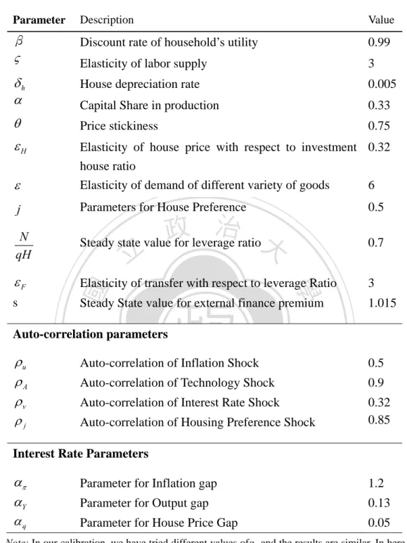
(19) the steady state equilibrium for the model.. 3. Calibration. 3.1 Parameters Setting. We follow Chen and Cheng (2012) for most of the parameters settings. The parameter settings are shown in Table 1. We set the discount factor in household ,β equals to be 0.99, and the elasticity. 政治大. of labor supply to be 3 as the setting in Aoki (2005). In our work, the elasticity of. 立. demand for different variety of goods is chosen to be 6 as the traditional setting, and. ‧ 國. 學. the price stickiness chosen to be 0.75 so that the representative retailer is likely to change its price every four periods. Also here the depreciation rate of house is fixed to. ‧. be 0.005 and the difference between marginal borrowing rate and real interest rate to. y. Nat. io. sit. be 0.015 according to the setting in Chen and Cheng (2012) . Furthermore, we set the. n. al. er. steady state of leverage ratio (the ratio between house owner net wealth and house. Ch. i Un. v. expenditure) to be 0.7, and the elasticity of house price with respect to investment. engchi. house ratio to be 0.32 as the setting in Chen and Cheng (2012). In addition, we choose the parameter for house preference to be 0.5. For the parameters of auto-correlation of exogenous variables, we follow the settings in Chen and Cheng (2012), and the parameter for monetary policy shock in our work is set to be 0.32. We also fix the parameters of technology shock and house demand shock to be 0.85 and 0.09, respectively. For the interest rate rule, we first follow the setting in Chen and Cheng (2012) and set the parameters of inflation gap and output gap to 1.2 and 0.13.. 14 .

(20) Table 1. Calibration Parameters. Parameter. Description. Value. β . Discount rate of household’s utility. 0.99. Elasticity of labor supply. 3. h . House depreciation rate. 0.005. Capital Share in production. 0.33. . Price stickiness. 0.75. H  . Elasticity of house price with respect to investment 0.32 house ratio Elasticity of demand of different variety of goods 6. j. Parameters for House Preference. 0.5. 治政 Steady state value for leverage ratio大立. 0.7. F . Elasticity of transfer with respect to leverage Ratio. 3. Steady State value for external finance premium. 1.015. ‧. ‧ 國. s. 學. N qH. Auto-correlation parameters. n. al. y er. Auto-correlation of Interest Rate Shock. sit. Auto-correlation of Technology Shock. io. j. Auto-correlation of Inflation Shock. Nat. u A v. i Un. v. Auto-correlation of Housing Preference Shock. Ch. Interest Rate Parameters. engchi. 0.5 0.9 0.32 0.85.  Y. Parameter for Inflation gap. 1.2. Parameter for Output gap. 0.13. q. Parameter for House Price Gap. 0.05. Note: In our calibration, we have tried different values ofαq and the results are similar. In here, we just show the result with the value 0.05.. 3.2 Calibration Results. In our calibration, we will compare the effect of a 1% inflation shock (cost-push), technology shock and interest rate shock under different interest rate rule. 15 .

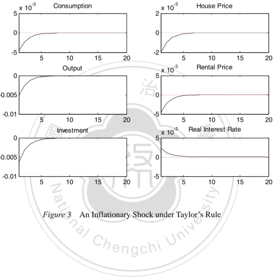
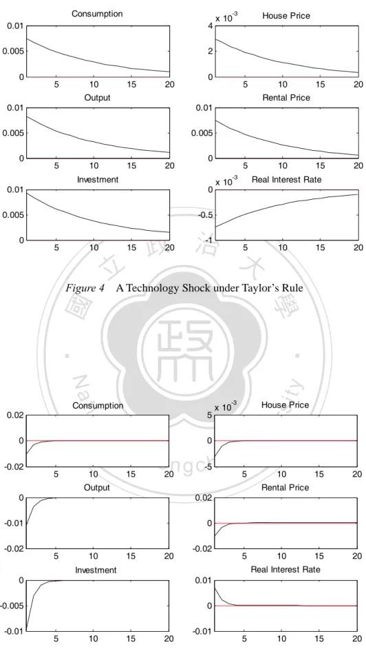
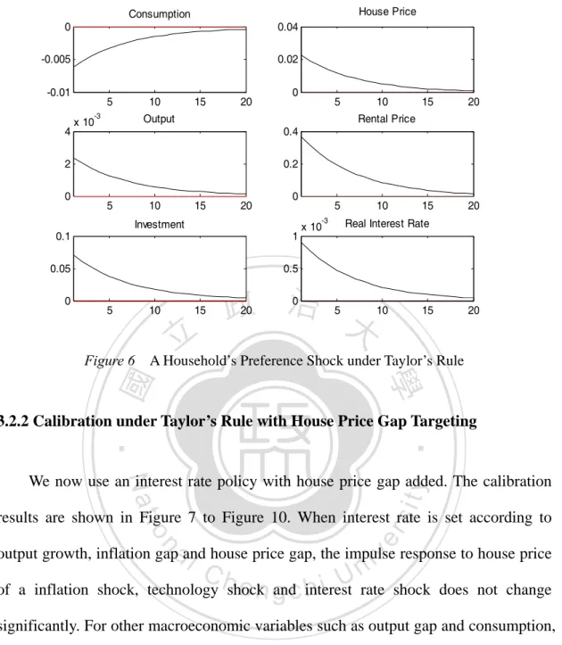
(21) 3.2.1 Calibration under Taylors Rule We first assume the authority set the interest rate under traditional Taylors Rule, as shown in (19). The results are shown as Figure 3 to Figure 6.A positive inflationary shock will cause the representative firm to decrease its output and lead to a decrease in labor demand and wage. With lower income, the representative household will decrease its consumption and house renting demand. This will decrease the house rental price and house owner’s house demand. The house price will decrease and the house investment will decrease as a result.. 政治大 income will increase as a result. With more income, the representative’s house renting 立. A positive technology shock will lead to an increase in output. The household’s. demand and consumption will increase. The rental price will increase and the house. ‧ 國. 學. owner‘s demand on houses will increase as well. Consequently, the house price will. ‧. increase, followed by an increase in house producer’s investment.. sit. y. Nat. A positive shock to interest rate will increase the opportunity cost of borrowing funds.. io. er. This will make buying houses more difficult for the representative house owner.. al. iv n C U decrease. Lower house price will lower incentive on investment h e ntheghouse c h iproducer’s n. Therefore, the house demand of representative household and the house price will. and cause a decrease in house investment. Also, an increase in interest rate will cause the representative household to save more money in period t and decrease his consumption. The decrease in consumption and house investment will cause a decrease in output and lead to a decrease in labor demand and real wage rate. An increase on household’s preference for houses will lead to higher demand on house renting for household. The house rental price will increase and cause the house price to rise consequently. Higher house price will lead to higher investment on houses. Also, since the representative household spends more on houses, there will be 16 .

(22) less consumption. In order to seek for more budgets on buying houses, consumer will increase its labor and lead to an increase on output along with the increased investment.. -3. 5. -3. Consumption. x 10. 2. 0 -5. 0. 5. 10. 15. 20. -2. 0. 5. 5. 10. 立. 15. 20. -5. 20. 10. 15. -5. 5. 10. An Inflationary Shock under Taylor’s Rule. n. al. er. io. sit. y. 20. ‧. ‧ 國. x 10. 0. Nat. 5. 5 -3. 5. Figure 3. Ch. engchi. 17 . 10 15 Real Interest Rate. x 10. 學. -0.01. 20. 0. Investment. -0.005. 10 15 Rental Price. 政治大. -0.005. 0. 5 -3. Output. -0.01. House Price. x 10. i Un. v. 15. 20.

(23) Consumption. -3. 0.01. 4. 0.005. 2. 0. 5. 10. 15. 0. 20. House Price. x 10. 5. 10. Output 0.01. 0.01. 0.005. 0.005. 0. 5. 10. 15. 0. 20. 0.01. 0. 0.005. -0.5. 5. 10. Figure 4. 5 -3. Investment. 0. 15. x 10. -1. 20. 10. 5. 10. ‧ 國 15. 0. e n g c-5h i 20. -0.01. 0. 10. 15. -0.02. 20. 5. 5. Investment 0.01. -0.005. 0. 10. Figure 5. 15. -0.01. 20. 10. 10. 5. 10. A Monetary Shock under Taylor’s Rule. 18 . 15. 20. v. Real Interest Rate. 0. 5. 20. sit. i Un. Rental Price 0.02. -0.01. 15. y. 10. Ch. House Price. x 10. Output. 5. 20. er. al. 0. -0.02. 15. ‧ -3. 5. n 5. 20. 學. io. -0.02. 15. 立A Technology Shock under Taylor’s Rule. Nat 0. 20. Real Interest Rate. 政治大. Consumption. 0.02. 15. Rental Price. 15. 20.

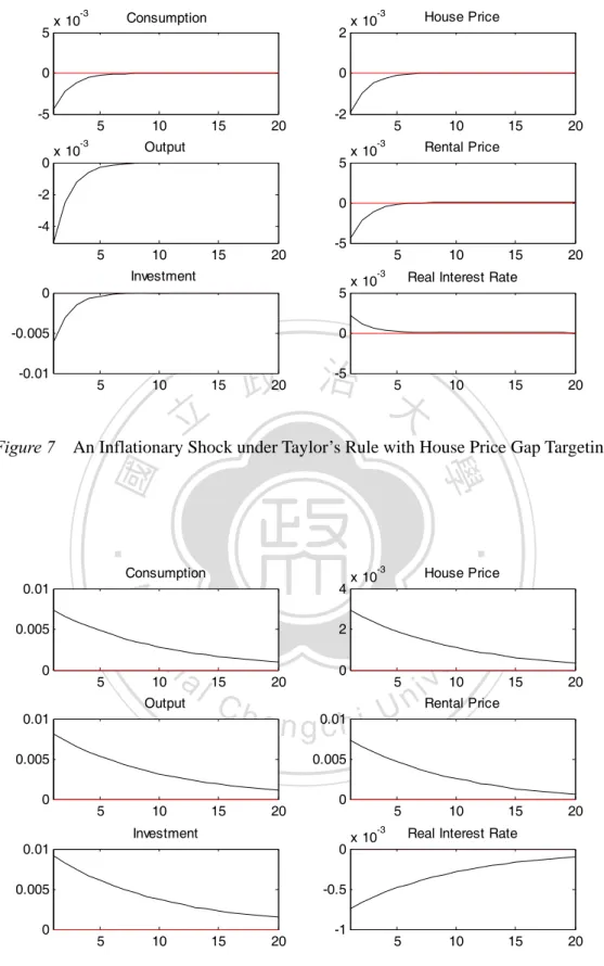
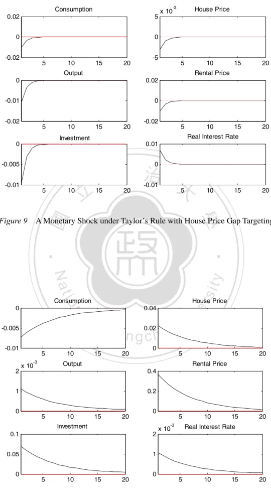
(24) House Price. Consumption 0. 0.04. -0.005. 0.02. -0.01. 5. 10. -3. 4. 15. x 10. 10. 15. 20. 15. 20. Rental Price 0.4 0.2. 5. 10. 15. 0. 20. 5 -3. Investment. 0.1. 1. 0.05 0. 5. Output. 2 0. 0. 20. 10. Real Interest Rate. x 10. 0.5. 5. 10. 15. 立. Figure 6. 政治大 0. 20. 5. 10. 15. 20. A Household’s Preference Shock under Taylor’s Rule. ‧ 國. 學. 3.2.2 Calibration under Taylor’s Rule with House Price Gap Targeting. ‧. Nat. sit. y. We now use an interest rate policy with house price gap added. The calibration. n. al. er. io. results are shown in Figure 7 to Figure 10. When interest rate is set according to. i Un. v. output growth, inflation gap and house price gap, the impulse response to house price. Ch. engchi. of a inflation shock, technology shock and interest rate shock does not change significantly. For other macroeconomic variables such as output gap and consumption, the change rate is similar with the one under Taylor’s Rule. Though the house price growth decrease a little in the preference shock, the decline is not significant as well. Therefore, adding house price gap into Taylor’s rule interest rate setting do not help in stabilizing house price significantly.. 19 .

(25) -3. 5. -3. Consumption. x 10. 2. 0. 0. -5. 5 -3. 0. House Price. x 10. 10. 15. -2. 20. x 10. 5. 10. -3. Output 5. -2. 15. 20. 15. 20. Rental Price. x 10. 0. -4 5. 10. 15. -5. 20. Investment 0. 5. -0.005. 0. 10. 15. 立. -5. 20. n. a l 15 Output Ch 10. y. sit. 0. 20. 5. e n g 0.01 chi U. 0.005. v 10 15 i n Rental Price. 20. 0.005. 5. 10. 15. 0. 20. 0.01. 0. 0.005. -0.5. 5. 10. 5 -3. Investment. 15. -1. 20. 10. 15. 20. Real Interest Rate. x 10. 5. 10. 15. 20. A Technology Shock under Taylor’s Rule with House Price Gap Targeting. 20 . 20. House Price. x 10. 2. io 5. 0.01. Figure 8. 15. ‧. 4. Nat. 0.005. 0. 10. 學 -3. Consumption. 0. 5. An Inflationary Shock under Taylor’s Rule with House Price Gap Targeting. 0.01. 0. x 10. 政治大. ‧ 國. Figure 7. 5. 10. Real Interest Rate. er. -0.01. 5 -3.

(26) -3. Consumption 0.02. 5. 0. 0. -0.02. 5. 10. 15. -5. 20. House Price. x 10. 5. 10. Output 0. 0.02. -0.01. 0. -0.02. 5. 10. 15. -0.02. 20. 5. 10. 20. 0. -0.01. 10. 立. 15. 政治大 -0.01. 20. 5. 10. ‧ sit. y. Nat 0.04. n. al. House Price. -0.005 -0.01. 5 -3. 10. Ch 15. i Un. 0.02. engchi 0. 20. 5. Output. x 10. v. 10. 15. 20. 15. 20. Rental Price 0.4. 1. 0.2. 5. 10. 15. 0. 20. Investment 2. 0.05. 1. 5. 10. 5 -3. 0.1. Figure 10. er. io. Consumption. 0. 20. A Monetary Shock under Taylor’s Rule with House Price Gap Targeting. 0. 0. 15. 學. ‧ 國. 5. Figure 9. 15. 0. 20. 10. Real Interest Rate. x 10. 5. 10. 15. 20. A Preference Shock under Taylor’s Rule with House Price Gap Targeting 21 . . 15. 0.01. -0.005. 2. 20. Real Interest Rate. Investment. 0. 15. Rental Price.

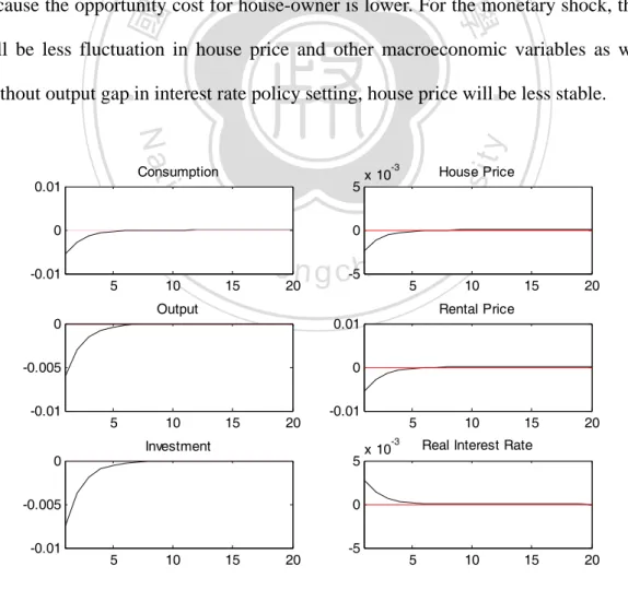
(27) 3.2.3 Calibration under Interest Rate Rule with Inflation Targeting Then, we set the monetary authority use an inflation targeting interest rule. The impulse response results of the three shocks are shown in Figure 11 to Figure 14. In the absence of output gap in interest rate rule, the effect on the economy is stronger. With a cost push shock (inflationary shock), the house price will decline more because the real interest rate rises when the decline of output is not taken into account in interest rate policy setting. The representative household will have more incentive in saving rather than consumption in period t with higher interest rate. Therefore,. 政治大 policy setting. The house price growth caused by an advance in technology is larger 立. consumption will decline more compared to the one with Taylor’s Rule interest rate. ‧ 國. 學. because the opportunity cost for house-owner is lower. For the monetary shock, there will be less fluctuation in house price and other macroeconomic variables as well.. ‧. Without output gap in interest rate policy setting, house price will be less stable.. 5. n 5. 10. Ch 15. e n g c-5h i 20. 5. 10. 15. 10. 15. 20. 15. 20. Rental Price. -0.01. 20. 5 -3. Investment. 5. -0.005. 10. Real Interest Rate. x 10. 0. 5. Figure 11. 10. 15. -5. 20. 5. 10. 15. An Inflationary Shock under Inflation Rate Targeting 22 . . v. 0. 0. -0.01. 5. 0.01. -0.005 -0.01. i Un. 0. Output. 0. House Price. x 10. er. io. al. sit. y. Nat. 0 -0.01. -3. Consumption. 0.01. 20.

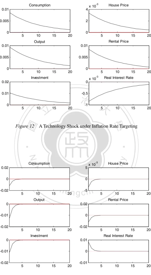
(28) -3. Consumption 0.01. 4. 0.005. 2. 5. 10. 15. 5. 10. 15. 0. 20. 0. 0.01. -0.5. 5. 10. 立. 15. 20. Real Interest Rate. x 10. -1. 20. 5. ‧ 國. io. 0. n. al. 10. Ch. 15. e20n g c-5h i. 20. y House Price. i Un 5. -0.01. 0. 10. 15. 20. -0.02. 5. Investment 0.01. -0.01. 0. Figure 13. 10. 15. 20. 10. 15. 20. Real Interest Rate. 0. 10. v. Rental Price 0.02. 5. 15. sit. 5. 0. 5. 10. ‧. Nat. -3. x 10. Output. 15. 20. -0.01. 5. 10. 15. A Monetary Shock under Inflation Rate Targeting. 23 . 15. A Technology Shock under Inflation Rate Targeting. 0. 5. 10. 政治大. Consumption. -0.02. 20. 學. Figure 12. 0.02. 5 -3. Investment. -0.02. 15. 0.005. 0.02. -0.02. 10. 0.01. 0.005. 0. 5. Rental Price. Output. 0.01. 0. 0. 20. er. 0. House Price. x 10. 20.

(29) Consumption. House Price. 0. 0.04. -0.005. 0.02. -0.01. 5 -3. 4. 10. 15. x 10. 10. 15. 20. 15. 20. Rental Price. 0.4 0.2. 5. 10. 15. 0. 20. Investment 1. 0.05. 0.5. 5. 10. Real Interest Rate. x 10. 政治大. 15. 0. 20. 立. 5. 10. 15. 20. A Preference Shock under Inflation Rate Targeting. ‧. ‧ 國. 10. 學. Figure 14. 5 -3. 0.1. 0. 5. Output. 2 0. 0. 20. We then change our interest rate rule into a more aggressive one as discussed in. Nat. sit. y. Bernanke and Getler (2000) by increasing the parameter for inflation target into 2.. n. al. er. io. The impulse response results are shown as in Figure 15 to Figure 18. The effect of an. i Un. v. inflationary shock on house price will be more severe because there will be larger. Ch. engchi. interest rate growth. For the monetary shock, with a more aggressive interest rate rule setting, the impulse shock on house price and other macroeconomic variables will be less strong. Therefore, whether an aggressive monetary policy works better in house price stabilization compared to an accommodating one (when the parameter for inflation gap is 1.2) is ambiguous.. 24 .

(30) Consumption. House Price. 0.02. 0.01. 0. 0. -0.02. 5. 10. 15. 20. -0.01. 5. 10. 15. 20. 10 15 Real Interest Rate. 20. Output. Rental Price. 0. 0.02. -0.01. 0. -0.02. 5. 10. 15. 20. -0.02. 5. Investment 0. 0.01. -0.01. 0. 5. 立. 15. 政治大 20. -0.01. y 4. n. al. 5. 10. sit. -3. Ch. 15. House Price. x 10. i Un. 2. e20n g c 0h i. 5. Output 0.01. 0.01. 0.005. 0.005. 5. 10. 15. 0. 20. 0. 0.01. -0.5. Figure 16. 10. 5 -3. 0.02. 5. v. 10. 15. 20. 15. 20. Rental Price. Investment. 15. -1. 20. 10. Real Interest Rate. x 10. 5. 10. 15. 20. A Technology Shock under Aggressive Inflation Rate Targeting 25 . . 20. er. io. 0.005. 0. 15. ‧. Nat. 0.01. 0. 10. An Inflationary Shock under Aggressive Inflation Rate Targeting. Consumption. 0. 5. 學. Figure 15. 10. ‧ 國. -0.02.

(31) -3. Consumption 0.01. 5. 0. 0. -0.01. 5. 10. 15. -5. 20. House Price. x 10. 5. 10. Output 0. 0.01. -0.005. 0. -0.01. 5. 10. 15. -0.01. 20. 0. 5. -0.005. 0. 5. 10. 15. 立. x 10. 政治大 -5. 20. 5. 10. ‧ 國. y. sit. n. al. House Price 0.04. 10. Ch 15. e n g c 0h i 20. 15. 20. 15. 20. 0.2. 5. 10. 15. 0. 20. 1. 0.05. 0.5. 5. 10. 5 -3. 0.1. Figure 18. 15. 0. 20. 10. Real Interest Rate. x 10. 5. 10. 15. 20. A Preference Shock under Aggressive Inflation Rate Targeting 26 . . 10. 0.4. Investment. 0. 5. v. Rental Price. 1 0. i Un. 0.02. Output. x 10. 20. er. io. 2. 15. ‧. Nat 5 -3. 20. A Monetary Shock under Aggressive Inflation Rate Targeting. -0.005 -0.01. 15. Rental Price. Consumption. 0. 20. 學. Figure 17. 10. 5 -3. Investment. -0.01. 15. Rental Price.

(32) 4. Conclusion In this paper, we compare the effect of various shocks on house price under different monetary policies by using the dynamic stochastic general equilibrium model (DSGE). In our model, we set up a house producer, a representative house owner, a representative household who rent houses from the house owner, a goods firm and a monetary authority (so-called “Central Bank”). We compute the steady state and linearize the model. We calibrate the impulse response of the macroeconomic variables with various shocks under a traditional Taylor’s Rule, an interest rate policy with house price gap added in traditional Taylor’s Rule and an. 治政 inflation targeting interest rate rule. Then, we calibrate 大 an aggressive inflation 立 targeting interest rate rule and compare with the accommodating one. We find out that ‧ 國. 學. adding house price gap into traditional Taylor’s Rule does not work better in house. ‧. price stabilization compared to traditional Taylor’s Rule. Also, through our calibration,. sit. y. Nat. we find out the importance of traditional Taylor’s Rule in stabilization of house price. io. er. and other macroeconomic variables. When the interest rate rule policy can react to an. al. n. economy’s output growth, the economy’s boom and bust will be eased off and there. ni C h market. will be less fluctuation in the housing U engchi. v. We conclude this paper by pointing out some related issues for future research. First, we can discuss the effect of different loan borrowing rate (the ratio that an individual is allowed to borrow for the house purchase) on house demand and house price. Also, we have discussed an economy in absence of fiscal policies. We can add some fiscal policies such as implementing a tax on return on buying houses. Furthermore, we can compare the effect of monetary policies and fiscal policies on house price stabilizing.. 27 .

(33) Reference Aoki, K., J. Proudman, and G. Vlieghe (2002), “House Prices, Consumption, and Monetary Policy: A Financial Accelerator Approach”, Bank of England Working Paper, 169-190. Bernanke, B. and M. Getler (1999), “Monetary Policy and Asset Price Volatility”, Economic Review, 4, 17-51. Bernanke, B., M. Getler, and S. Gilchrist (1999), “The Financial Accelerator in a Quantitative Business Cycle Framework”, Handbook of Macroeconomics, 1, 1341-1393.. 政治大. Central Bank of China (Taiwan) (2013), Meeting of Board of Central Bank Committee (News Announcement No 130), Retrieved from http://www.cbc.gov.tw/ ct.asp?xItem=44416&ctNode=302&mp=1.. 立. ‧ 國. 學. ‧. Central Bank of China (Taiwan) (2014), The International Perspective on House Price, Interest Rate and Cautious Policies, Retrieved from http://www.cbc.gov.tw/ public/Attachment/422416342071.pdf.. y. Nat. sit. n. al. er. io. Chang, C. O., M. C. Chen, H. J. Teng, and C.Y. Yang (2009), “Is There a Housing Bubble in Taipei? Housing Price vs. Rent and Housing Price vs. Income”, Journal of Housing Studies, 18(2), 1-22.. Ch. engchi. i Un. v. Chen, N. K. and H. L. Cheng (2012), “External Finance Premium, Taiwan’s Housing Market and Business Fluctuations”, Economic Thesis, Institute of Economics, Academic Sinica, 40(3), 307–341. SinYi Research Center for Real Estate (2014), Taiwanese House Price Index (Data file). Retrieved from the website of National ChengChi University College of Commerce: https://www.ncscre.nccu.edu.tw/webroot/xponent/exponent_ 1314260174.docx. Iacoviello, M. (2005), “House Prices, Borrowing Constraints, and Monetary Policy in the Business Cycle”, American Economic Review, 95(3), 739-764.. 28 .

(34) Lin, T. Y. (2012), “Monetary Policy and the House Price” (No. 100-2410-H-004-198), Ministry of Science and Technology, Taiwan: Taipei City, Retrieved from http://nccur.lib.nccu.edu.tw/bitstream/140.119/52370/1/100-2410-H-004-198.pdf. Taiwanese Economic Journal (2014), Taiwanese House Price to Income Ratio (Database). Retrieved from Taiwanese Economic Journal Database.. 立. 政治大. ‧. ‧ 國. 學. n. er. io. sit. y. Nat. al. Ch. engchi. 29 . i Un. v.

(35) Appendix. Linearization. (A) Household.    Ct  Et Ct 1  Rt. .. (A1).    wt  Ct   Lt. ... (A2).     H t  jt  xth  Ct. ... (A3). (B) House owner. 立. (A4). .. 學. ‧ 國.     bbt 1  qH (qt  H t 1 )  NNt 1. 政治大.  (1   h )  xh   Rth1  Et [ h xth1  qt 1  qt ] h qR R h  R qH  h   bsR   Fh h Nt  ( Rt  qt 1  H t )  (bt  Rt )  Ft N N N     Ft h   F ( N t 1  qt  H t 1 ). .. ‧. (A6). .. y. (A7) (A8). io. n. al. sit. Nat.   Rth1  Rt. Ch. (C) House Producer. n engchi U.    H t   h I th  (1   h ) H t 1. (A5). er. .. iv. .. (A9). ..    qt   H ( I th  H t 1 ). ... (A10). .. (A11). (D) Goods Firm . .  t   Et t 1 . (1   )(1   )   mc t  ut. .    Yt  At  (1   t ) Lt. ... 30 . (A12).

(36)    t  w mc t  Lt  Yt. .. (A13). (E) Market Clearing  C  I h h Yt  Ct + I t Y Y. .. (A14). The monetary policies and exogenous shocks are as listed in Section 2.6 and Section 2.7.. 立. 政治大. ‧. ‧ 國. 學. n. er. io. sit. y. Nat. al. Ch. engchi. 31 . i Un. v.

(37)