三維Poisson方程在圓柱及球座標下之形式四階緊緻差分法

全文

(1)國立交通大學應用數學系碩士論文. 三維 Poisson 方程在圓柱及球座標下之形式四階緊緻差分法 A formally fourth-order compact scheme for Poisson equation in cylindrical and spherical coordinates. 研究生：曾瑞閔指導老師：賴明治. 教授. 中華民國九十五年一月.

(2) 三維 Poisson 方程在圓柱及球座標下之形式四階緊緻差分法 A formally fourth-order compact scheme for Poisson equation in cylindrical and spherical coordinates 研究生：曾瑞閔. Student：Jui-Ming Tsung. 指導教授：賴明治. Advisor：Ming-Chih Lai. 國立交通大學應用數學系碩士論文. A Thesis Submitted to Department of Applied Mathematics College of Science National Chiao Tung University in Partial Fulfillment of the Requirements for the Degree of Master in Applied Mathematics January 2006 Hsinchu, Taiwan, Republic of China. 中華民國九十五年一月.

(3) 三維 Poisson 方程在圓柱及球座標下之形式四階緊緻差分法學生：曾瑞閔. 指導老師：賴明治教授. 國立交通大學應用數學系(研究所)碩士班. 摘. 要. 在這篇論文裡，將會介紹三維 Poisson 方程在圓柱及球座標下簡單且有效率的四階緊緻解法。這個解法是由截斷 (truncated)傅利葉級數展開式所產生，且得到一組傅利葉係數所形成的偏微分方程組，運用緊緻差分技巧，我們可以得到四階精確且不需奇異點條件的結果。接著利用兩種有效的迭代法(GMRES,BI-CGSTAB)來解離散後，傅利葉係數所形成非對稱的線性系統並配合不同的 preconditioner。. i.

(4) A formally fourth-order compact scheme for Poisson equation in cylindrical and spherical coordinates Student：Jui-Ming Tseng. Advisors：Dr. Ming-Chih Lai. Department﹙Institute﹚of Applied Mathematics National Chiao Tung University ABSTRACT A simple and efficient compact fourth-order Poisson solver in cylindrical and spherical coordinates is presented. The solver relies on the truncated Fourier series expansion, where the differential equations of Fourier coefficients have been solved by fourth-order finite difference discretizations without pole conditions. And two kinds of efficient iterative method, GMRES and Bi-CGSTAB, with different preconditioners are applied to solve the resulted nonsymmetrical systems of Fourier coefficients.. ii.

(5) 誌謝研究所求學過程中，承蒙指導教授賴明治老師於學業與論文上的教誨，使學生在學術研究、待人處事與生涯規劃上受益良多，並讓本論文得以順利完成，學生在此謹致最誠摯的謝意。口試期間，承蒙吳金典教授、黃聰明教授及張書銘教授費心審閱並提供許多寶貴之意見，使本論文之完稿得以更加齊備，永誌於心。由衷感謝父母親多年來無悔的養育與教導之恩，以及家人的照顧與關心，使我無後顧之憂的順利完成碩士學位。此外，在研究所求學過程中十分感謝研究室成員--曾昱豪學長、同學和學弟妹於課業上的協助與日常生活上的關懷與鼓勵，在此一併獻上誠摯感謝之意。最後，謹將本論文之研究成果獻給我敬愛的父母親、家人以及所有關心我的人，共同分享這份喜悅與榮耀。. -iii-.

(6) 目中文提要英文提要誌謝目錄 1、 2、 2.1 2.2 3、 3.1 3.2 4、 5、 6、 7、參考文獻. 錄. ……………………………………………………………… ……………………………………………………………… ……………………………………………………………… ……………………………………………………………… Introduction Fast Poisson solver in cylindrical coordinates Fourier mode equations Fourth-order finite difference discretization Fast Poisson solver in spherical coordinates Fourier mode equations Fourth-order finite difference discretization Generalized Minimal Residual (GMRES) Bi-Conjugate Gradient Stabilized (Bi-CGSATB) The compact fourth-order scheme on polar geometry with Neumann problems Conclusions ………………………………………………………………. iv. i ii iii iv 1 2 2 3 12 13 14 21 26 33 39 39.

(7) 1. Introduction. In many physical problems, one often needs to solve the Poisson equation on a non-Cartesian domain, such as polar or cylindrical or spherical domains. It is convenient to rewrite the equation in those coordinates. The …rst problem that must be dealt with is the coordinate singularities caused by the transformation. The singularities occur at the polar axis of those domains. It is important to note that the occurrence of those singularities is due to the representation of the governing equation in those coordinates. Most of …nite di¤erence, …nite volume and spectral methods in the literature (see Lai & Wang, 2002) need to either approximate the value of the solution or impose appropriate pole conditions for the solution at the singularities. This pole approximation provides a numerical boundary value for the …nite di¤erence scheme. In Lai (2002), the author developed FFT-based fast direct solvers for Poisson equation on 2D polar geometry. The author uses the truncated Fourier series expansion to derive a set of singular ODEs for the Fourier coe¢ cients, and then solves those singular equations by the compact fourth-order …nite di¤erence discretizations. By shifting a half mesh width from the origin, and incorporating with the derived symmetry constraint of Fourier coe¢ cients, we can easily handle coordinate singularities without pole conditions. By manipulating the radial mesh width, three di¤erent boundary problems for polar geometry (Dirichlet, Neumann and Robin conditions) can be solved equally easily. In this paper, we extend the previous fourth-order schemes on two dimensional cases (Lai, 2002) to the three-dimensional domains. Using the truncated Fourier series expansion, the original three-dimensional PDE now becomes a set of two-dimensional PDEs of the Fourier coe¢ cients. Then we solve those PDEs by fourth-order …nite di¤erence discretizations. In the following, we present two kinds of iterative method, GMRES and Bi-CGSTAB, to solve the nonsymmetric systems of two-dimensional PDEs of Fourier coe¢ cients. Then some preconditioners can be used. In particular, a preconditioner arising from those singular equations have been solved by the second-order …nite di¤erence discrtizations (see Lai et al, 2002) and shown to be the most e¢ cient one.. 1.

(8) 2. Fast Poisson solver in cylindrical coordinates. The Poisson equation on a cylinder = f0 < r 1; 0 can be conveniently written in cylindrical coordinates as. < 2 ;0. z. 1g. @ 2 u 1 @u 1 @2u @2u + + + 2 = f (r; z; ) (2.1) @r2 r @r r2 @ 2 @z For the sake of simplicity, we restrict the Dirichlet boundary conditions on the top and bottom boundaries, u(r; 1; ) = uT (r; ), u(r; 0; ) = uB (r; ), but consider three di¤erent type of sidewall boundary conditions: Dirichlet u(1; z; ) = uS (z; ); Neumann @u (1; z; ) = uS (z; ); or Robin condition @r @u + u(1; z; ) = u (z; ); > 0. S @r The main issue for solving Eq.(2.1) is how to treat the coordinate singularity along the polar axis at the center r = 0. Most of Poisson solvers for Eq.(2.1) including …nite di¤erence and spectral methods (see Chen et al: (2000), Lai & Wang (2002)), involve imposing additional pole conditions to approximate accurately the solution in the vicinity of the origin. The accuracy of those methods depends greatly on the choice of pole conditions. In the following, we develop a new class of fast direct solver for Eq.(2.1). Our approach relies on the truncated Fourier series expansion, where the di¤erential equations of Fourier coe¢ cients are solved by the fourth-order …nite di¤erence discretizations without pole condition.. 2.1. Fourier mode equations. Since the solution u is periodic in , we can approximate it by the truncated Fourier series as N=2 1. u(r; z; ) =. X. u^n (r; z) ein ;. (2.2). n= N=2. where u^n (r; z) is the complex Fourier coe¢ cient given by. and. N 1 1 X u^n (r; z) = u(r; z; N k=0. k. k) e. in. k. ;. = 2k =N , and N is the number of grid points along a circle. 2. (2.3).

(9) Substituting the expansions of (2.2) into Eq.(2.1), and equating the Fourier coe¢ cients, we derive u^n (r; z) satisfying the PDE @ 2 u^n 1 @ u^n @ 2 u^n + + @r2 r @r @z 2. n2 u^n = f^n (r; z); 0 < r r2. 1; 0. z. 1;. (2.4). where the nth Fourier coe¢ cient of the right-hand side function f^n (r; z) is de…ned similarly as (2.3). The Fourier coe¢ cients of the boundary values u^nS (z), u^nT (r), u^nB (r) are also de…ned in a similar fashion as to (2.3). So the remaining problem is to solve Eq.(2.4) with the top and bottom boundary conditions u^n (r; 0) = u^nB (r), u^n (r; 1) = u^nT (r), and with one of the three u ^n u ^n sidewall boundary conditions u^n (1; z) = u^nS (z), @@r (1; z) = u^nS (z), or @@r + n u^n (1; z) = u^S (z).. 2.2. Fourth-order …nite di¤ erence discretization. We choose a grid in (r; z) plane to avoid the polar singularity by ri = (i. 1=2) r;. zj = j. z;. (2.5). for 1 i L + 1; 0 j M + 1, with r = 2=(2L + 1) and z = 1=(M + 1). Let the discrete values be denoted by U (ri ; zj ) u^n (ri ; zj ), ^ F (ri ; zj ) fn (ri ; zj ). Our goal is to derive a fourth-order …nite di¤erence approximation to Eq.(2.4). Obviously, the …rst and second derivatives, Ur , Urr and Uzz , must be approximated to fourth-order accurately. First, let us write down two di¤erence formulas for the …rst and second derivatives with the truncation errors O( r4 ) and O( z 4 ): Ur =. 0(r) Uij. r2 Urrr + O( r4 ); 6. (2.6). Urr =. 2 (r) Uij. r2 Urrrr + O( r4 ); 12. (2.7). Uzz =. 2 (z) Uij. z2 Uzzzz + O( z 4 ): 12. (2.8). 3.

(10) Here 0(r) Uij , 2(r) Uij and 2(z) Uij are the centered di¤erence operators for the …rst and second derivatives, de…ned as 0(r) Uij. =. Ui+1;j Ui 2 r. 1;j. ;. 2 (r) Uij. =. Ui+1;j. 2Ui;j + Ui r2. 1;j. ;. 2 Ui;j + Ui;j 1 ; (2.9) z2 where Ui;j are the discrete values de…ned at the grid points ri and zj . In order to have fourth-order approximations for Ur , Urr and Uzz , we need to approximate the higher order derivatives Urrr , Urrrr and Uzzzz in Eqs.(2.6) , (2.7) and (2.8) to be second-order accurate. To accomplish this, we di¤erentiate Eq.(2.4) once and twice for radial and axial directions, respectively, to obtain the higher order derivatives of U : 2 (z) Uij. Urrr Urrrr. Uzzz Uzzzz. =. Ui;j+1. Urr 1 + n2 2n2 = Fr + Ur U Uzzr ; r r2 r3 Fr 3 + n2 3 + 5n2 8n2 Uzzr = Frr + U U + U+ rr r 2 3 4 r r r r r Uzzrr ; Urz n2 = Fz Urrz + 2 Uz ; r r Urzz n2 = Fzz Urrzz + 2 Uzz : r r. (2.10). (2.11) (2.12) (2.13). In Eqs.(2:10) , (2:11) , (2:12) , (2:13), those di¤erential operators in righthand side can be approximated further by the centered di¤erence formulas to achieve second-order accuracy. Substituting those approximations into Eqs.(2.6) , (2.7) and (2.8) then applying to Eq.(2.4), we obtain the …nite di¤erence scheme as follows. For 1 i L; 1 j M , we need to solve 2 (r) Ui;j. r2 [ 12. 8n2 1 + 4 Ui;j + ri ri 1 ri. 2 (r) Ui;j. 2 (r) Fi;j. 1 ri. 2 0(r) (z) Ui;j. 1 + n2 + ri2. 0(r) Ui;j. 0(r) Fi;j +. 3 + n2 ri2. 2 2 (r) (z) Ui;j ]. 2n2 Ui;j ri3 4. 1 + ri. 2 (r) Ui;j. 0(r) Ui;j. 2 0(r) (z) Ui;j ]. 3 + 5n2 ri3 r2 [ 6ri. 0(r) Ui;j. 0(r) Fi;j. n2 Ui;j + ri2. 2 (z) Ui;j.

(11) z2 [ 12. 2 (z) Fi;j. 1 ri. 2 2 (z) (r) Ui;j. 2 (z) 0(r) Ui;j. +. n2 ri2. 2 (z) Ui;j ]. = Fi;j :. (2.14). In order to close the linear system, the numerical boundary values U0;j and UL+1;j in the r direction should be supplied. Choosing of ri as described in (2.5), we have rL+1 = 1; thus, the numerical boundary value UL+1;j can either be given by the Dirichlet boundary value u^nS (zj ) or be determined by imposing the condition on the boundary (Neumann and Robin). The numerical boundary value U0;j can be obtained by the symmetry constraint of Fourier coe¢ cients, which is derived as follows. The transformation between Cartesian and cylindrical coordinates can be written as x = r cos ; y = r sin ; z = z. When we replace r with r, and with + , the Cartesian coordinates of a point remain the same. Therefore, any scalar function u(r; ; z) satis…es u( r; ; z) = u(r; + ; z). Using this equality, we have u( r; ; z) =. 1 X. in. u^n ( r; z) e. 1 X. =. n= 1. =. 1 X. u^n (r; z) ein(. + ). n= 1 in. u^n (r; z) e. in. e. =. n= 1. 1 X. ( 1)n u^n (r; z) ein :. (2.15). n= 1. Thus, when the domain of a function is extended to a negative value of r, the nth Fourier coe¢ cient of this function satis…es u^n ( r; z) = ( 1)n u^n (r; z). Using the above condition, we have U0;j = U (r0; zj ) = U (. r r ; zj ) = ( 1)n U ( ; zj ) 2 2. = ( 1)n U (r1; zj ) = ( 1)n U1;j :. (2.16). Therefore, the numerical boundary value U0;j has been supplied. And the numerical boundary values in the z direction can be easily obtained by the given Dirichlet boundary values Ui;0 = u^nB (ri ) and Ui;M +1 = u^nT (ri ). Let us order the unknowns Uij by …rst grouping the same i so that the solution vector v is de…ned by 2 3 2 3 U1 Ui1 6 U2 7 6 Ui2 7 6 7 6 7 v = 6 .. 7 ; Ui = 6 .. 7 : 4 . 5 4 . 5 UL UiM 5.

(12) Solving the discrete equations (2.14) results in a large sparse linear system Av = b, where the coe¢ cient matrix A and the right-hand side vector b are de…ned as follows. The matrix A is a L L block tridiagonal matrix 2 3 T1 I1 6 H2 T2 I2 7 6 7 6 7 : : : 7; A=6 6 7 : : : 6 7 4 HL 1 TL 1 IL 1 5 HL TL where Ti ; Hi and Ii ; 1 2. i. H1i 6 H2i 6 6 Hi = 6 6 6 4 5a 6 a = + 12 2. b (1 + n2 )ci 6 b ei fi ; 12. 5a 6 a = + 12. b (1 + n2 )ci + (1 + 3n2 )di 6 b + ei + fi ; 12. H1i = H2i. L are the tridiagonal matrices given by 3 H2i 7 H1i H2i 7 7 : : : 7; 7 : : : 7 H2i H1i H2i 5 H2i H1i (1 + 3n2 )di + 2ei. I1i I2i 6 I2i I1i I2i 6 6 : : : Ii = 6 6 : : : 6 4 I2i I2i I2i I2i I1i. I1i = I2i. 6. 10fi ;. 3. 7 7 7 7; 7 7 5 2ei + 10fi ;.

(13) 2. Ti. T1. 3. T 1i T 2i 6 T 2i T 1i T 2i 6 6 : : : = 6 6 : : : 6 4 T 2i T 1i T 2i T 2i T 1i n = T1 + ( 1) H11 I; T 1i = T 2i =. 5a 5b + 2(1 3 3 a 5b + n2 ci ; 6 6. 4n2 )ci. 7 7 7 7; 7 7 5. n2 gi ;. 2. r r 1 1 with a = 1r2 ; b = 1z2 ; ci = 12r ; gi = 3rr4 . 2 ; di = 24r 3 ; ei = 24r 2 ; fi = 24r i z i r i i i Incorporating with the boundary values and the function F , the right-hand side vector b can be written as 2 3 bT1;j 7 6 bT2;j 7 6 b=6 7; .. 5 4 .. bTL;j. I1L u^nS (Zj ). I2L (^ unS (Zj 1 ) + u^nS (Zj+1 )). where. bi;j =. bL;j =. 8 > > > > < > > > > :. 8 > > > > > < > > > > > :. Fi+1;j + H2i u^nB (ri i Fi+1;j + i Fi+1;j + H2i u^nT (ri i. L FL+1;j. 1) i Fi i Fi 1). F. F. 2F. + i;j12 1 + 3i;j + i;j+1 12 T 2i u^nB (ri ) I2i u^nB (ri+1 ) Fi;j 1 2Fi;j Fi;j+1 1;j + 12 + 12 + 3 Fi;j+1 Fi;j 1 2Fi;j 1;j + 12 + 12 + 3 T 2i u^nT (ri ) I2i u^nT (ri+1 ). i Fi 1;j. + L FL 1;j H2L u^nB (rL L FL+1;j + L FL 1;j L FL+1;j + L FL 1;j H2L u^nT (rL. F. F. 1 + L;j+1 + L;j + 12 12 n ) T 2 u ^ (r ) 1 L B L F F 1 + L;j+1 + L;j + 12 12 FL;j+1 FL;j 1 + 12 + 12 + T 2L u^nT (rL ) 1). if j = 1 if 2. j. if j = M. 2FL;j 3 2FL;j 3 2FL;j 3. 1 ;. M. if j = 1 if 2. j. M. 1 ;. if j = M. 1 1 i with i = 12 + 12i ; i = 12 ; i = 2rri ; 1 i L. 12 Note that, the above form is for the Dirichlet sidewall boundary. We shall discuss the other cases below.. 7.

(14) For the Neumann ( = 0) or Robin boundary cases, we use the same mesh points but with di¤erent radial mesh width r = 1=L. With this choice of radial mesh width, the discrete values of U are de…ned midway between sidewall boundary so that the …rst derivative can be centered on the grid points. That is, at r = 1, @U + U @r. UL+1;j. UL;j r. UL+1;j + UL;j = u^nS (zj ): 2. +. (2.17). The numerical boundary value UL+1;j can be approximated by UL+1;j =. (1. r=2)UL;j + u^nS (zj ) r : 1+ r=2. (2.18). Therefore, we only need to modify TL in the matrix A and bTL;j in the vector b by TL = TL + IL ; bTL;j = bTL;j (I1L u^nS (Zj ). I2L (^ unS (Zj 1 ) 1. + r. u^nS (Zj+1 ))). (2.19) b1 ;(2.20) T. with b1 = I2L (^ unB (rL ); 0; :::; 0; u^nT (rL )); = 1+ 2r and = 1+ r r . 2 2 Table 2.1 shows the maximum errors of the method for three di¤erent solutions of Poisson equation in a cylinder with Dirichlet boundary condition. In all our tests, we use L mesh points in the radial and axial directions, and 2L points in the azimuthal direction. The rate of convergence is computed E by the formula log2 ( EL=2 ), where EL is the maximum error. One can see that L the errors of the solutions show third-order convergence for all solutions. The loss of one order of accuracy seems to come from the discretization near the origin. This can be seen from the following truncation error analysis. In 0 u ^n the Fourier mode equation Eq.(2.4), the U (= @@r ) term is divided by r. 000 So the second-order approximation of U in (2.6) is divided by an O( r) 000 term near the origin, which makes the approximation of U =r …rst-order accurate. This has the consequence that the overall truncation error of the 0 U =r term in the vicinity of the origin is O( r3 ) and thus so is the Fourier mode equation (2.4). However, this loss of accuracy does not appear when solving the problem on a hollow cylinder. Let us explain why that is the case next. The present scheme can be easily applied to solve the Poisson equation on a hollow cylinder fa r bg, where a > 0. As the cylinder case, we need 8.

(15) to solve Eq.(2.4) and three di¤erent boundary conditions at r = b with an additional boundary condition imposed at r = a. Instead of setting a grid as in (2.5), we choose a regular grid, ri = a + i r; i = 0; 1; 2; :::; L; L + 1;. (2.21). with the mesh width r = (b a)=(L + 1). Now the second-order approxi000 mation of U in (2.6) is divided by an O(a + r) term instead of an O( r) 0 term, so the truncation error of the U =r term is still O( r2 ). Therefore, the overall truncation error of Eq.(2.4) is O( r4 ). The fourth and …fth columns of Table 2.1 show the errors and the rate of convergence for the solutions on a hollow cylinder f0:5 r 1g. We can see that the fourth-order convergence can be achieved for all examples. In the following, the Table 2.2 and 2.3 show the maximum errors of the method for three di¤erent solutions of Poisson equation in a cylinder and hollow cylinder with remaining boundary conditions(Neumann and Robin).. 9.

(16) Table 2.1 The Maximum Errors of Di¤erent Solutions to the Poisson Equation with Dirichlet Boundary 0<r 1 0:5 < r 1 L kuk1 Rate kuk1 Rate u(r; z; ) = er cos 8 7.8137E-05 16 9.8506E-06 32 1.2566E-06 64 1.5941E-07. +r sin +z. u(r; z; ) = r3 (cos 8 9.1438E-04 16 1.0755E-04 32 1.3008E-05 64 1.5966E-06. 1.5465E-07 1.0920E-08 7.3409E-10 4.7580E-11. 3.82 3.90 3.95. + sin )z(1 z) 8.8994E-07 3.09 6.4128E-08 3.05 4.3173E-09 3.03 2.8035E-10. 3.80 3.89 3.95. 2.99 2.97 2.98. u(r; z; ) = cos( (r2 cos2 + r sin )) sin( 8 7.4000E-03 7.5000E-03 16 3.3150E-04 4.48 1.7101E-05 32 4.0782E-05 3.02 1.2221E-06 64 5.0424E-06 3.02 8.1011E-08. 10. z2) 8.78 3.81 3.92.

(17) Table 2.2 The Maximum Errors of Di¤erent Solutions to the Poisson Equation with Neumann Boundary 0<r 1 0:5 < r 1 L kuk1 Rate kuk1 Rate u(r; z; ) = er cos 8 4.2863E-04 16 1.0817E-04 32 2.6993E-05 64 6.7313E-06. +r sin +z. u(r; z; ) = r3 (cos 8 1.4000E-03 16 3.5261E-04 32 8.8215E-05 64 2.2041E-05. 9.3911E-05 2.4471E-05 6.2247E-06 1.5682E-06. 1.94 1.96 1.99. + sin )z(1 z) 2.9138E-04 1.99 7.7016E-05 2.00 1.9828E-05 2.00 5.0323E-06. 1.92 1.96 1.99. 1.99 2.00 2.00. u(r; z; ) = cos( (r2 cos2 + r sin )) sin( 8 2.4900E-02 2.0200E-02 16 4.1000E-03 2.60 1.1000E-03 32 1.1000E-03 1.90 2.8932E-04 64 3.0123E-04 1.87 7.5139E-05. 11. z2) 4.20 1.93 1.95.

(18) Table 2.3 The Maximum Errors of Di¤erent Solutions to the Poisson Equation with Robin Boundary ( = 1) 0<r 1 0:5 < r 1 L kuk1 Rate kuk1 Rate u(r; z; ) = er cos 8 1.0000E-03 16 2.5937E-04 32 6.4653E-05 64 1.6112E-05. +r sin +z. u(r; z; ) = r3 (cos 8 4.2000E-03 16 1.0000E-03 32 2.6050E-04 64 6.5035E-05. 2.3024E-04 5.9649E-05 1.5131E-05 3.8114E-06. 1.95 1.98 1.99. + sin )z(1 z) 8.7050E-04 2.07 2.3109E-04 1.94 5.9561E-05 2.00 1.5121E-05. 1.91 1.96 1.98. 1.95 2.00 2.00. u(r; z; ) = cos( (r2 cos2 + r sin )) sin( 8 2.3100E-02 1.9100E-02 16 5.3000E-03 2.12 1.3000E-03 32 1.6000E-03 1.73 3.9232E-04 64 4.1390E-04 1.95 1.0176E-04. 3. z2) 3.88 1.73 1.95. Fast Poisson solver in spherical coordinates. The Poisson equation in a spherical shell = fR0 2 g can be written in spherical coordinates as. r. 1; 0. @ 2 u 2 @u 1 @ 2 u cot @u 1 @2u + + + + = f (r; ; ): @r2 r @r r2 @ 2 r2 @ r2 sin2 @ 2. ;0. (3.1). The boundary condition should be imposed on the inner (r = R0 > 0) and outer (r = 1) surfaces of the sphere. Here, for convenience of exposition, we assume the Dirichlet boundary on the inner surface u(R0 ; ; ) = uI ( ; ). Three di¤erent boundary conditions can be considered on the outer surface: Dirichlet u(1; ; ) = uS ( ; ); Neumann @u (1; ; ) = uS ( ; ); or Robin @r condition @u + u(1; ; ) = u ( ; ); > 0. However, the method to be S @r 12.

(19) described can be easily adapted to di¤erent boundary conditions on the inner surface. As in the cylindrical case of the previous section, the main di¢ culty for solving Eq.(3.1) is to treat the coordinate singularities along the polar axis where north ( = 0) and south ( = ) poles are located. Again, most of numerical approaches including …nite di¤erence and spectral methods involve imposing additional pole conditions to capture the behavior of the solution in the vicinity of the poles. In the following, we will present a numerical method to solve Eq.(3.1) which uses the symmetry constraint of Fourier coe¢ cient to handle the coordinate singularities without pole condition.. 3.1. Fourier mode equations. As in the cylindrical coordinate case, we approximate u by the truncated Fourier series as N=2 1. u(r; ; ) =. X. u^n (r; ) ein ;. (3.2). n= N=2. where u^n (r; ) is the complex Fourier coe¢ cient given by N 1 1 X u(r; ; u^n (r; ) = N k=0. k) e. in. k. ;. (3.3). and k = 2k =N and N is the number of grid points along a latitude circle. The expansion for the function f can be written in the similar fashion. Substituting those expansions into Eq.(3.1), and equating the Fourier coe¢ cients, u^n (r; ) then satis…es the PDE 1 @ 2 u^n cot @ u^n @ 2 u^n 2 @ u^n + + + 2 @r2 r @r r2 @ 2 r @. n2 u^n = f^n (r; ); r2 sin2. (3.4). with u^n (R0 ; ) = u^nI ( ) and one of the three boundary conditions: Dirichlet u ^n u ^n u^n (1; ) = u^nS ( ); Neumann @@r (1; ) = u^nS ( ); or Robin condition @@r + u^n (1; ) = u^nS ( ). Here, u^nI ( ) and u^nS ( ) are the nth Fourier coe¢ cient of uI ( ; ) and uS ( ; ), respectively.. 13.

(20) Fourth-order …nite di¤ erence discretization. 3.2. We consider the Dirichlet boundary on the outer surface …rst and will discuss the other cases later. Let us choose a grid in (r; ) plane by ri = R0 + i r;. j. = (j. 1=2). (3.5). ;. for 0 i L+1; 0 j M +1 with r = (1 R0 )=(L+1) and = =M . By the choice of those mesh points, we avoid placing points directly at north ( = 0) and south ( = ) poles. Again, let the discrete values be denoted by U (ri ; j ) u^n (ri ; j ), and F (ri ; j ) f^n (ri ; j ). Our goal is to derive a fourth-order …nite di¤erence approximation to Eq.(3.4). As in the cylindrical coordinate case, we obtain the …nite di¤erence scheme as follows. For 1 i L; 1 j M , we need to solve. 2 (r) Ui;j. +(. +. 6 ri3 2 ri 1 ri2. 8. r2 [ 12. 2 ri. 2 (r) Fi;j. 6n2 csc2 ri3. j. ). cot ri2. 2 2 (r) Ui;j +(. + n2 csc2 ri2. +((3+n2 ) csc2. j 2 (r) 0(. 2n2 csc2 ri3. +( 3 5n2 ) csc2. j. j. cot. 1). 10 ri4. 0(r) Ui;j. 2 0(r) ( ) Ui;j. 2 0(r) ( ) Ui;j. 0(r) Fi;j + (. j. ). j. 8 + n2 csc2 ri2. 2 ( ) Ui;j. U ) i;j. 1 ri2. 0(r) Ui;j +. 2 2 ( ) Ui;j +ri. cot. 2 2 (r) (. 2 cot ri3. 1 Ui;j ]g+ 2 f ri. j 0( ) Ui;j +2n. 10 cot ri4. 2. ). j. 2 (r) Ui;j. j. +. 0( ) Ui;j +. 2 U ]+ f i;j ) ri. 10n2 csc2 ri4. 6 cot ri3. j. j. Ui;j. 0(r) 0( ) Ui;j. r2 [ 6. 0(r) Ui;j. 2 2 0( ) Ui;j + 3 ( ) Ui;j ri. 0(r) Fi;j. cot ri2. j. 0(r) 0( ) Ui;j. 2 2 ( ) Ui;j. csc2. 12. j (4 csc. 2 j 0( ) (r) Ui;j. 14. j. [ri2. 2 j. 2ri. 2 ( ) Fi;j. ri2 cot. 3)Ui;j +2ri cot. 2 ( ) 0(r) Ui;j. ri2. j 0( ) Fi;j. j 0( ) 0(r) Ui;j. 2 2 ( ) (r) Ui;j ]g.

(21) cot j + 2 f ri. 2 0( ) Ui;j. 6. [ ri2. 2 2 2 0( ) (r) Ui;j +(1+n ) csc. j 0( ) Ui;j. cot. 2 j ( ) Ui;j. n2 csc2 j Ui;j = Fi;j : (3.6) 0( ri2 When j = 1 for Eq.(3.6), the numerical boundary value Ui;0 can be given by Ui;0 = ( 1)n Ui;1 . This is because the Fourier coe¢ cient satis…es the symmetry constraint u^n (ri ; =2) = ( 1)n u^n (ri ; =2) (Lai & Wang, 2002). Similarly, another numerical boundary value Ui;M +1 can also be obtained by Ui;M +1 = ( 1)n Ui;M for the same reason. So the numerical boundary values in the direction are provided and no pole condition is needed in our …nite di¤erence setting. The numerical boundary values in the radial direction U0;j ; UL+1;j are given by the boundary values u^nI ( j ); u^nS ( j ). Let us order the unknowns Uij by …rst grouping the same i so that the solution vector v is de…ned by 2 3 2 3 U1 Ui1 6 U2 7 6 Ui2 7 6 7 6 7 v = 6 .. 7 ; Ui = 6 .. 7 : 4 . 5 4 . 5 UL UiM 2n2 csc2. j cot. 2 j Ui;j + ri. ) Fi;j ]g. The remaining problem is to solve a large sparse linear system Av = b, where the coe¢ cient matrix A and the right-hand side vector b are de…ned as follows. The matrix A is a L L block tridiagonal matrix 2 3 T1 I1 6 H2 T2 I2 7 6 7 6 7; : : : A=6 7 4 HL 1 TL 1 IL 1 5 HL TL. where Ti ; Hi and Ii ; 1 i L are the tridiagonal matrices given by 2 T 1i;1 + ( 1)n T 3i;1 T 2i;1 6 T 3i;2 T 1i;2 T 2i;2 6 6 : : : Ti = 6 6 : : : 6 4 T 3i;M 1 T 1i;M 1 T 2i;M 1 T 3i;M T 1i;M + ( 1)n T 2i;M 15. 3. 7 7 7 7; 7 7 5.

(22) T 1i;j =. 20P 1 8P 3i;j P 7i;j P 8i;j +2. 2. P 3i;j 2P 9i 10P 6i +P 10i;j +. 2. P 6i ;. 2 P 10i;j P 3i;j P 6i +P 11i;j +P 12i;j +P 13i;j P 14j 2P 1; 2 2 2 P 10i;j P 3i;j P 6i P 11i;j P 12i;j P 13i;j +P 14j 2P 1; T 3i;j = P 9i +5P 6i 2 2 2 H1i;1 + ( 1)n H3i;1 H2i;1 6 H3i;2 H1i;2 H2i;2 6 6 : : : Hi = 6 6 : : : 6 4 H3i;M 1 H1i;M 1 H2i;M 1 H3i;M H1i;M + ( 1)n H2i;M. T 2i;j = P 9i +5P 6i. H1i;j = 10P 1 H2i;j = P 15i;j H3i;j =. P 15i;j. 10P 2i. P 3i;j. P 4i;j. 2P 5i P 6i ; P 12i;j P 14j P 6i + + + P 1; P 16i;j + P 5i P 2i + 10 2 2 P 14j P 6i P 12i;j + + P 1; + P 16i;j + P 5i P 2i 10 2 2. 2. I1i;1 + ( 1)n I3i;1 I2i;1 6 I3i;2 I1i;2 I2i;2 6 6 : : : Ii = 6 6 : : 6 4 I3i;M I1i;j = 10P 1 + 10P 2i I2i;j =. P 15i;j. I3i;j = P 15i;j. 3 : 1. I1i;M 1 I2i;M 1 I3i;M I1i;M + ( 1)n I2i;M. P 3i;j + P 4i;j + 2P 5i P 6i ; P 12i;j P 14j P 6i + P 16i;j P 5i + P 2i + + + + P 1; 10 2 2 P 12i;j P 14j P 6i P 16i;j P 5i + P 2i + + P 1; 10 2 2. 16. 7 7 7 7; 7 7 5. 3. 7 7 7 7; 7 7 5.

(23) with P1 = P 5i = P 8i;j = P 11i;j = P 14j =. n2 csc2 j rn2 csc2 j 1 ; P 2i = ; P 3i;j = ; P 4i;j = ; 12 r2 12ri r 12ri2 12ri3 r2 n2 csc2 j r 1 ; P 6 = ; P 7 = ; i i;j 6ri4 12ri3 2 6ri2 2 2 2 csc2 j n csc4 j r2 ; P 9 = ; ; P 10 = i i;j 3ri2 6ri2 6ri4 2 r2 cot j 5 cot j (1 + 3n2 )( cot j csc2 ; P 12i;j = ; P 13i;j = 12ri4 12ri2 24ri2 cot j r cot j cot j ; P 15i;j = ; P 16i;j = ; 1 j M: 3 2 12 r 24ri 24ri r 1. j). Incorporating with the boundary value and the function F , the right-hand side vector b can be written as 3 2 T b1;j H31;j u^nI ( j 1 ) H11;j u^nI ( j ) H21;j u^nI ( j+1 ) .. 7 6 . 7 6 7 6 T bi;j b=6 7; 7 6 . .. 5 4 T n n n bL;j I3M;j u^s ( j 1 ) I1M;j u^s ( j ) I2M;j u^s ( j+1 ) where bi;j =. 2 1 1 Fi;j + ( + P 17i )Fi+1;j + ( 3 12 12 1 r2 P 14j 1 )Fi;j+1 + ( +( + 12 2 12. P 17i )Fi. 1;j. r2 P 14j )Fi;j 1 ; 2. with P 17i = 12rri ; 1 i L and 1 j M . For the Neumann ( = 0) or Robin boundary cases, we use the same grid described in (3.5) but with di¤erent radial mesh width r = 2(1 R0 )=(2L+ 1). With this choice of radial mesh width, the discrete values of U are de…ned midway between boundary so that the …rst derivative can be centered on the mesh points. That is, at r = 1, @U + U @r. UL+1;j. UL;j r. + 17. UL+1;j + UL;j = u^nS ( j ): 2. (3.7). ;.

(24) So the numerical boundary value UL+1;j can be approximated by UL+1;j =. r=2)UL;j + u^nS ( j ) r : 1+ r=2. (1. (3.8). Therefore, we only need to modify TL in the matrix A and the vector bTL;j by TL = TL + IL ; bTL;j = bTL;j (I3M;j u^ns ( 1. (3.9) j 1). r. I1M;j u^ns ( j ). I2M;j u^ns ( j+1 ));(3.10). with = 1+ r r ; and = 1+ 2r . 2 2 Table 3.1 shows the maximum errors of the method for three di¤erent solutions of Poisson equation in a spherical shell with Dirichlet boundary condition. In all our tests, we use L mesh points in the radial and colatitude directions, and 2L points in the longitude direction. The inner radius is chosen by R0 = 0:5. One can see that the errors of the solutions show third-order convergence for all solutions. The loss of one order of accuracy seems to come from the discretization near the north ( = 0) pole. This can be seen from the following truncation error analysis. In the Fourier mode equation Eq.(3.4), 0 the U (= @@u^n ) term is divided by sin . So the fourth-order approximation of 0 U in (3.4) is divided by an O( ) term near the north ( = 0) pole. This has 0 U term in the the consequence that the overall truncation error of the cot r2 vicinity of the north ( = 0) pole is O( 3 ) and thus so is the Fourier mode equation (3.4). In the following, the Table 3.2 and 3.3 show the maximum errors of the method for three di¤erent solutions of Poisson equation in a spherical shell with remaining boundary conditions(Neumann and Robin).. 18.

(25) Table 3.1 The Maximum Errors of Di¤erent Solutions to the Poisson Equation with Dirichlet Boundary 0:5 < r 1 L kuk1 Rate u(r; ; ) = er sin cos +r sin 8 3.7000E-03 16 5.4095E-04 32 7.4825E-05 64 1.0067E-05. sin +r cos. 2.77 2.85 2.89. u(r; ; ) = r3 (cos + sin ) sin (1 8 5.2000E-03 16 9.5143E-04 32 1.5249E-04 64 2.2549E-05 u(r; ; ) = cos( (r2 cos2 sin2 8 5.3700E-02 16 7.1000E-03 32 8.3568E-04 64 9.7240E-05. 19. r cos ) 2.45 2.64 2.76. + r sin sin )) sin( r2 cos2 ) 2.92 3.09 3.10.

(26) Table 3.2 The Maximum Errors of Di¤erent Solutions to the Poisson Equation with Neumann Boundary 0:5 < r 1 L kuk1 Rate u(r; ; ) = er sin cos +r sin 8 6.8000E-03 16 8.5296E-04 32 1.0804E-04 64 1.4317E-05. sin +r cos. 3.00 2.98 2.92. u(r; ; ) = r3 (cos + sin ) sin (1 8 1.0500E-02 16 1.6000E-03 32 2.2105E-04 64 2.9431E-05 u(r; ; ) = cos( (r2 cos2 sin2 8 1.3090E-01 16 1.6500E-02 32 2.2000E-03 64 3.8002E-04. 20. r cos ) 2.71 2.86 2.91. + r sin sin )) sin( r2 cos2 ) 2.99 2.91 2.53.

(27) Table 3.3 The Maximum Errors of Di¤erent Solutions to the Poisson Equation with Robin Boundary ( = 1) 0:5 < r 1 L kuk1 Rate u(r; ; ) = er sin cos +r sin 8 6.0000E-03 16 8.0381E-04 32 1.0805E-04 64 1.5225E-05. sin +r cos. 2.90 2.90 2.83. u(r; ; ) = r3 (cos + sin ) sin (1 8 9.6000E-03 16 1.5000E-03 32 2.1788E-04 64 3.3247E-05 u(r; ; ) = cos( (r2 cos2 sin2 8 1.0880E-01 16 1.2900E-02 32 1.6000E-03 64 2.4752E-04. 4. r cos ) 2.68 2.78 2.71. + r sin sin )) sin( r2 cos2 ) 3.08 3.01 2.69. Generalized Minimal Residual (GMRES). In this section, we present an iterative method for solving nonsymmetric linear systems of the Fourier mode equation (2.4). The Generalized Minimal Residual (GMRES) method is an extension of MINRES (which is only applicable to symmetric systems) to nonsymmetric linear systems(see Saad and Schultz). The stopping criterion of the convergence is based on the relative residual which the tolerance ranges from 10 12 10 16 depending on the di¤erent Fourier modes. In the Conjugate Gradient method, the residuals form an orthogonal basis for the space span r(0) ; Ar(0) ; A2 r(0) ; ::: . In GMRES, this orthonormal basis is formed explicitly:. 21.

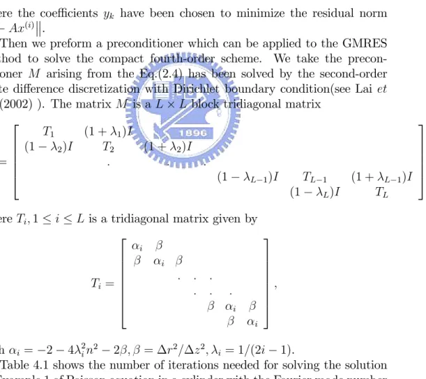
(28) ! (i) = Av (i) for k = 1; :::; i ! (i) = ! (i). (! (i) ; v (k) )v (k). end v (i+1) = ! (i) = ! (i) The reader may recognize this as a modi…ed Gram-Schmidt orthogonalization. The GMRES iterates are constructed as x(i) = x(0) + y1 v (1) + ::: + yi v (i) ;. (4.1). where the coe¢ cients yk have been chosen to minimize the residual norm b Ax(i) . Then we preform a preconditioner which can be applied to the GMRES method to solve the compact fourth-order scheme. We take the preconditioner M arising from the Eq.(2.4) has been solved by the second-order …nite di¤erence discretization with Dirichlet boundary condition(see Lai et al: (2002) ). The matrix M is a L L block tridiagonal matrix 2 T1 (1 + 1 )I 6 (1 T2 (1 + 2 )I 2 )I 6 6 : : : M =6 4 (1 TL 1 (1 + L 1 )I L 1 )I (1 TL L )I where Ti ; 1. i. L is a tridiagonal matrix given by 2 3 6 6 6 Ti = 6 6 6 4. i. i. :. : :. : :. : i i. 7 7 7 7; 7 7 5. with i = 2 4 2i n2 2 ; = r2 = z 2 ; i = 1=(2i 1). Table 4.1 shows the number of iterations needed for solving the solution of Example 1 of Poisson equation in a cylinder with the Fourier mode number n = 1 and Dirichlet boundary condition by GMRES method with di¤erent 22. 3. 7 7 7; 7 5.

(29) preconditioners. The tolerance for the relative residual is chosen as 10 13 . Those preconditioners include block Jacobi (BJ), incomplete LU factorization (LUINC), and the fast Poisson solver (FPS) described as before. Indeed, the fast Poisson solver preconditioner turns out to be the most e¢ cient one since it has the least number of iterations, and the iterations are kept to be a constant when we increase the grid points. Table 4.1 The performance comparison for using di¤erent preconditioners 0<r 1 u(r; z; ) = er cos +r sin +z L Outer/Inner Iteration Relative residual Tolerance Relative Error. 8 16 32 64. 8 16 32 64. 8 16 32 64. 8 16 32 64. 1/38 1/74 1/145 2/1. GMRES 4.2482E-14 8.7889E-14 8.3080E-14 9.6686E-14. 1.0E-13 1.0E-13 1.0E-13 1.0E-13. 7.8137E-05 9.8506E-06 1.2566E-06 1.5941E-07. 1/25 1/48 1/90 1/164. BJ 2.5087E-14 5.4973E-14 6.7025E-14 8.5684E-14. 1.0E-13 1.0E-13 1.0E-13 1.0E-13. 7.8137E-05 9.8507E-06 1.2565E-06 1.5909E-07. 1/10 1/16 1/27 1/47. LUINC 1.2748E-14 2.1491E-14 3.7427E-14 7.4488E-14. 1.0E-13 1.0E-13 1.0E-13 1.0E-13. 7.8137E-05 9.8505E-06 1.2566E-06 1.5913E-07. 1/15 1/15 1/15 2/1. (2-order)FPS 1.5611E-14 5.0064E-14 2.7255E-14 2.4130E-14. 1.0E-13 1.0E-13 1.0E-13 1.0E-13. 7.8137E-05 9.8506E-06 1.2566E-06 1.5941E-07. 23.

(30) In the following, Table 4.2 and 4.3 show the number of iterations needed for solving the solution of remaining examples with the Fourier mode number n = 1 by GMRES method with di¤erent preconditioners. The tolerance for the relative residual is chosen as 10 13 . Similarly, the fast Poisson solver preconditioner turns out to be the most e¢ cient one since it has the least number of iterations, and the iterations are kept to be a constant when we increase the grid points. Table 4.2 The performance comparison for using di¤erent preconditioners 0<r 1 u(r; z; ) = r3 (cos + sin )z(1 z) L Outer/Inner Iteration Relative residual Tolerance Relative Error. 8 16 32 64. 1/28 1/58 1/115 2/1. GMRES 1.0713E-14 7.3844E-14 8.7476E-14 9.5299E-14. 8 16 32 64. 1/19 1/36 1/67 1/125. BJ 5.6023E-14 7.6266E-14 7.0556E-14 6.3349E-14. 1.0E-13 1.0E-13 1.0E-13 1.0E-13. 9.1438E-04 1.0755E-04 1.3008E-05 1.5966E-06. 8 16 32 64. 1/10 1/15 1/26 1/45. LUINC 2.1958E-14 6.7705E-14 5.5145E-14 6.0695E-14. 1.0E-13 1.0E-13 1.0E-13 1.0E-13. 9.1438E-04 1.0755E-04 1.3008E-05 1.5966E-06. 1/13 1/12 1/12 1/11. (2-order)FPS 1.4886E-14 7.5673E-14 2.3112E-14 1.9006E-14. 1.0E-13 1.0E-13 1.0E-13 1.0E-13. 9.1438E-04 1.0755E-04 1.3008E-05 1.5966E-06. 8 16 32 64. 24. 1.0E-13 1.0E-13 1.0E-13 1.0E-13. 9.1438E-04 1.0755E-04 1.3008E-05 1.5966E-06.

(31) Table 4.3 The performance comparison for using di¤erent preconditioners 0<r 1 u(r; z; ) = r2 sin 2 sin( z) L Outer/Inner Iteration Relative residual Tolerance Relative Error. 8 16 32 64. 1/35 1/69 1/136 1/267. GMRES 6.2341E-14 7.0950E-14 8.1227E-14 9.4758E-14. 8 16 32 64. 1/22 1/43 1/79 1/143. BJ 6.8349E-14 6.1935E-14 7.4148E-14 8.8186E-14. 1.0E-13 1.0E-13 1.0E-13 1.0E-13. 3.0938E-05 2.0650E-06 1.3481E-07 8.6030E-09. 8 16 32 64. 1/10 1/15 1/26 1/44. LUINC 2.0703E-14 6.1446E-14 7.2626E-14 7.6683E-14. 1.0E-13 1.0E-13 1.0E-13 1.0E-13. 3.0938E-05 2.0650E-06 1.3481E-07 8.6124E-09. 8 16 32 64. 1/13 1/13 1/13 1/13. (2-order)FPS 1.5440E-14 3.2524E-14 1.7154E-14 2.3399E-14. 1.0E-13 1.0E-13 1.0E-13 1.0E-13. 3.0938E-05 2.0650E-06 1.3481E-07 8.6031E-09. 25. 1.0E-13 1.0E-13 1.0E-13 1.0E-13. 3.0938E-05 2.0650E-06 1.3481E-07 8.6033E-09.

(32) 5. Bi-Conjugate Gradient Stabilized. In this section, we present the other e¢ cient iterative method for solving nonsymmetric linear systems. The stopping criterion of the convergence is based on the relative residual which the tolerance ranges from 10 9 10 13 depending on the di¤erent Fourier modes.First, we present the Conjugate Gradient Squared (CG-S) algorithm that was developed by Sonneveld (1984), mainly to avoid using the transpose of A in the Bi-Conjugate Gradient (Bi-CG) method and to gain faster convergence for roughly the same computational cost. In the Bi-CG algorithm, the approximations are constructed in such a way that the residual vector r(j) is orthogonal with respect to another vectors r~(0) ; r~(1) ; :::; r~(j 1) , and, vice versa, r~(j) is orthogonal with respect to r(0) ; r(1) ; :::; r(j 1) . Sonneveld observed that, in the case of convergence, both the rows r(j) and r~(j) converge to zero, but that only the convergence of the r(j) is used. He proposes the following modi…cation to Bi-CG by which all the convergence e¤ort is focused in the r(j) vectors. For the Bi-CG vectors it is well known that they can be written as r(j) = Pj (A)r(0) and r~(j) = Pj (AT )~ r(0) , and because of the bi-orthogonality relation we have that (r(j) ; r~(i) ) = (Pj (A)r(0) ; Pi (AT )~ r(0) ) = (Pi (A)Pj (A)r(0) ; r~(0) ) = 0 for i < j:. (5.1). The iteration parameters for Bi-CG are computed from innerproducts like the above. Sonneveld observed that we can also construct the vectors r^(j) = Pj2 (A)r(0) , using only the latter form of the innerproduct for recovering the Bi-CG parameters. By doing so, it can be avoided that the vectors r~(j) have to be formed, nor is here any multiplication with the matrix AT . The resulting algorithm can be represented by the following scheme M is a preconditioning matrix.. 26.

(33) PRECONDITIONED CG-S ALGORITHM — — — — Compute r(0) = b. Ax(0) for some initial guess x(0). r~(0) is an arbitrary vector, such that (r(0) ; r~(0) ) 6= 0, e.g.,r(0) = r~(0) ; for i = 1; 2; ::: i 1. if. = (~ r(0) ; r(i. 1). ). = 0 method fails. i 1. if i = 1 u(1) = r(0) p(1) = u(1) else i 1. =. i 1= i 2. u(i) = r(i. 1). +. p(i) = u(i) +. i 1q. i 1 (q. (i 1). (i 1). +. i 1p. (i 1). ). end if Solve p^ from M p^ = p(i) v^ = A^ p i. =. r(0) ; v^) i 1 =(~. q (i) = u(i). ^ iv. Solve u^ from M u^ = u(i) + q (i) x(i) = x(i. 1). +. ^ iu. q^ = A^ u r(i) = r(i. 1). ^ iq. check convergence; continue if necessary end. 27.

(34) The CG-S algorithm is based on squaring the residual polynomial, and, in case of irregular convergence, this may lead to a great quantity increasing of rounding errors, or possibly even over‡ow. The Bi-Conjugate Gradient Stabilized (Bi-CGSTAB) algorithm is a variation of CG-S which was developed to treat this di¢ culty (see Van der Vorst). Instead of seeking a method which expresses a residual vector of the form r^(j) , Bi-CGSTAB produces iterates whose residual are of the form r^(j) = Qj (A)Pj (A)r(0) ;. (5.2). in which, as before, Pj (t) is the residual polynomial associate with the Bi-CG algorithm and Qj (t) is a new polynomial which is de…ned recursively at each step with the goal of "stabilizing" or"smoothing" the convergence behavior of the original algorithm. The resulting algorithm can be represented by the following scheme. M is a preconditioning matrix. PRECONDITIONED Bi-CGSTAB ALGORITHM — — — — Compute r(0) = b. Ax(0) for some initial guess x(0). r~(0) is an arbitrary vector, such that (r(0) ; r~(0) ) 6= 0, e.g.,r(0) = r~(0) ; for i = 1; 2; ::: i 1. if. = (~ r(0) ; r(i. 1). ). = 0 method fails. i 1. if i = 1 p(i) = r(i. 1). else i 1. =(. p(i) = r(i. i 1 = i 2 )( i 1 =! i 1 ) 1). +. i 1 (p. (i 1). end if Solve p^ from M p^ = p(i) v (i) = A^ p i. =. r(0) ; v (i) ) i 1 =(~. s = r(i. 1). iv. (i). 28. ! i 1 v (i. 1). ).

(35) check norm of s; if small enough: set x(i) = x(i. 1). +. ^ ip. and. stop Solve s^ from M s^ = s t = A^ s ! i = (s; t)=(t; t) x(i) = x(i. 1). r(i) = s. !it. +. ^(i) ip. + ! i s^. check convergence; continue if necessary for continuation it is necessary that ! i 6= 0. end. Table 5.1 shows the number of iterations needed for solving the solution of Example 1 of Poisson equation in a cylinder with the Fourier mode number n = 1 and Dirichlet boundary condition by Bi-CGSTAB method with di¤erent preconditioners. The tolerance for the relative residual is chosen as 10 10 . Those preconditioners have been described in earlier section. Indeed, the fast Poisson solver preconditioner turns out to be the most e¢ cient one since it has the least number of iterations, and the iterations are kept to be a constant when we increase the grid points.. 29.

(36) Table 5.1 The performance comparison for using di¤erent preconditioners 0<r 1 u(r; z; ) = er cos +r sin +z L Iteration number Relative residual Tolerance Relative Error. 8 16 32 64. 25 52 97 182. Bi-CGSTAB 2.3263E-11 8.3558E-11 8.2703E-11 9.9557E-11. 8 16 32 64. 16 34 65 134. BJ 3.0152E-11 4.6514E-11 7.5701E-11 8.0676E-11. 1.0E-10 1.0E-10 1.0E-10 1.0E-10. 7.8136E-05 9.8505E-06 1.2564E-06 1.5885E-07. 8 16 32 64. 6 9 19 38. LUINC 1.8371E-11 7.8271E-11 3.6401E-11 7.1583E-11. 1.0E-10 1.0E-10 1.0E-10 1.0E-10. 7.8136E-05 9.8503E-06 1.2575E-06 1.6127E-07. 8 16 32 64. 7 7 7 7. (2-order)FPS 4.7806E-11 1.0E-10 6.9638E-11 1.0E-10 6.5055E-11 1.0E-10 2.7534E-11 1.0E-10. 7.8137E-05 9.8505E-06 1.2566E-06 1.5950E-07. 30. 1.0E-10 1.0E-10 1.0E-10 1.0E-10. 7.8136E-05 9.8507E-06 1.2564E-06 1.5835E-07.

(37) In the following, Table 5.2 and 5.3 show the number of iterations needed for solving the solution of remaining examples with the Fourier mode number n = 1 by Bi-CGSTAB method with di¤erent preconditioners. The tolerance for the relative residual is chosen as 10 10 . Similarly, the fast Poisson solver preconditioner turns out to be the most e¢ cient one since it has the least number of iterations, and the iterations are kept to be a constant when we increase the grid points. Table 5.2 The performance comparison for using di¤erent preconditioners 0<r 1 u(r; z; ) = r3 (cos + sin )z(1 z) L Iteration number Relative residual Tolerance Relative Error. 8 16 32 64. 17 34 67 138. Bi-CGSTAB 7.1236E-11 6.7664E-11 6.9265E-11 9.2923E-11. 8 16 32 64. 12 25 54 109. BJ 6.2911E-11 5.2211E-11 8.9216E-11 8.3574E-11. 1.0E-10 1.0E-10 1.0E-10 1.0E-10. 9.1438E-04 1.0755E-04 1.3008E-05 1.5966E-06. 8 16 32 64. 6 10 18 35. LUINC 1.0459E-11 1.5875E-11 7.2357E-11 7.2622E-11. 1.0E-10 1.0E-10 1.0E-10 1.0E-10. 9.1438E-04 1.0755E-04 1.3008E-05 1.5966E-06. 6 5 5 5. (2-order)FPS 2.2892E-11 1.0E-10 5.1414E-11 1.0E-10 5.5197E-11 1.0E-10 2.0837E-11 1.0E-10. 9.1438E-04 1.0755E-04 1.3008E-05 1.5966E-06. 8 16 32 64. 31. 1.0E-10 1.0E-10 1.0E-10 1.0E-10. 9.1438E-04 1.0755E-04 1.3008E-05 1.5966E-06.

(38) Table 5.3 The performance comparison for using di¤erent preconditioners 0<r 1 u(r; z; ) = r2 sin 2 sin( z) L Iteration number Relative residual Tolerance Relative Error. 8 16 32 64. 21 40 77 171. Bi-CGSTAB 5.5726E-11 8.3996E-11 8.2066E-11 8.9168E-11. 8 16 32 64. 15 32 62 114. BJ 1.0410E-11 9.1358E-11 9.9962E-11 9.5901E-11. 1.0E-10 1.0E-10 1.0E-10 1.0E-10. 3.0938E-05 2.0650E-06 1.3481E-07 8.6033E-09. 8 16 32 64. 6 10 18 35. LUINC 5.8224E-12 2.1490E-11 9.4662E-11 6.6702E-11. 1.0E-10 1.0E-10 1.0E-10 1.0E-10. 3.0938E-05 2.0650E-06 1.3481E-07 8.5840E-09. 8 16 32 64. 6 6 6 6. (2-order)FPS 1.1841E-11 1.0E-10 7.6716E-11 1.0E-10 6.6982E-11 1.0E-10 3.4051E-11 1.0E-10. 3.0938E-05 2.0650E-06 1.3481E-07 8.6042E-09. 32. 1.0E-10 1.0E-10 1.0E-10 1.0E-10. 3.0938E-05 2.0650E-06 1.3480E-07 8.5930E-09.

(39) 6. The compact fourth-order scheme on polar geometry with Neumann problems. In Lai (2002), the author present a simple and e¢ cient compact fourth-order Poisson solver in polar coordinates with Dirichlet problem. In this section, we will present the compact fourth-order scheme on polar geometry with di¤erent Neumann problems. The …rst, we consider a Neumann problem for the Poisson equation on a unit disk: 1 @2u @ 2 u 1 @u + + = f (r; ); 0 < r < 1; 0 @r2 r @r r2 @ 2. <2 ;. (6.1). @u (1; ) = g( ): (6.2) @r Since the solution u is periodic in , we can approximate it by the truncated Fourier series as N=2 1. u(r; ) =. X. u^n (r) ein ;. (6.3). n= N=2. where u^n (r) is the complex Fourier coe¢ cient given by N 1 1 X u^n (r) = u(r; N k=0. k) e. in. k. ;. (6.4). and k = 2k =N , and N is the number of grid points along a circle. Substituting those expansions into Eq.(6.1), and equating the Fourier coe¢ cients, we derive u^n (r) satisfying the ODE d2 u^n 1 d^ un n 2 + u^n = f^n ; 0 < r < 1; dr2 r dr r2 d^ un (1) = g^n ; dr. (6.5) (6.6). where f^n (r) and g^n are de…ned in a manner similar to that of (6.3) and (6.4). For the Neumann boundary, we choose a grid to avoid the polar singularity by ri = (i. 1=2) r; i = 0; 1; :::; M + 2; 33. (6.7).

(40) with r = 2=(2M + 1). Let the discrete values be denoted by U (ri ) u^n (ri ), F (ri ) f^n (ri ). By the same method that described in second section, we obtain the …nite di¤erence scheme as follows. For 1 i M + 1, we need to solve Ui. r2 2 ( Fi 12. 1 ri. 0 Ui. r ( 0 Fi 6ri. 1 ri. 2. +. 1 ri. +. 3 + n2 ri2. Ui +. 1 + n2 ri2. 0 Fi. 2. 2. Ui. 0 Ui. 3 + 5n2 ri3 2n2 Ui ) ri3. 0 Ui. +. 8n2 Ui ) ri4. n2 Ui = Fi : ri2. (6.8). The inner numerical boundary value U0 = ( 1)n U1 can be obtained by the symmetry constraint of Fourier coe¢ cients as before. And the outer numerical boundary value UM +2 is derived as follows. That is, at r = 1, 000. U r2 + O( r4 ) 0U = U + 6 00 r2 0 U 1 + n2 0 0 = U + (F + U 6 r r2 0. 2n2 U ) + O( r4 ): r3. UM +2 UM r2 3FM +1 4FM + FM = g^n + ( 2 r 6 2 r + (1 + n2 )^ gn 2n2 UM +1 ):. 1. UM +2. 2UM +1 + UM r2 (6.9). The outer numerical boundary value UM +2 can be approximated by UM +2 = (. 6 r 3 r 6 + r2 (1 + n2 ) r )[( )UM + ( )^ gn + FM +1 3+ r 6 r 6 4 r r 1 n2 r 2 FM + FM 1 + ( )UM +1 ]: (6.10) 3 12 3. Table 6.1 shows the maximum errors of this method for three di¤erent solutions of Poisson equation in unit disk with Neumann boundary condition at r = 1.. 34.

(41) Table 6.1 The Maximum Errors of Di¤erent Solutions to the Poisson Equation with Neumann Boundary @u (1; ) = g( ) using N = 64: @r 0<r 1 M kuk1 Rate u(x; y) = ex+y 16 4.2008E-05 32 5.3993E-06 64 6.8285E-07 128 8.5733E-08. 2.960 2.983 2.994. u(x; y) = 3ex+y (x 16 2.4161E-04 32 1.7289E-05 64 1.1573E-06 128 7.4875E-08 x. x2 )(y. y2) + 5. 3.805 3.901 3.950. y. +e u(x; y) = e1+xy 16 7.2000E-03 32 5.7732E-04 64 4.1560E-05 128 2.8026E-06. 3.641 3.796 3.890. The second, we consider a Neumann problem for the Poisson equation on an annulus: @ 2 u 1 @u 1 @2u + + = f (r; ); 0:5 < r < 1; 0 @r2 r @r r2 @ 2. <2 ;. (6.11). @u (1; ) = g( ): @r. (6.12). ri = 0:5 + i r; i = 0; 1; :::; M + 2;. (6.13). u(0:5; ) = k( ); We choose a regular grid,. with r = 1=(2M + 2). The …nite di¤erence scheme can be obtained as Eq.(6.8). Similarly, the outer numerical boundary value UM +2 can be approximated by (6:10). Table 35.

(42) 6.2 shows the maximum errors of this method for three di¤erent solutions of Poisson equation in an annulus with Neumann boundary condition at r = 1. Table 6.2 The Maximum Errors of Di¤erent Solutions to the Poisson Equation with Neumann Boundary u(0:5; ) = k( ); @u (1; ) = g( ) using N = 64: @r 0:5 r 1 M kuk1 Rate u(x; y) = ex+y 16 5.3054E-07 32 3.7859E-08 64 2.5324E-09 128 1.6362E-10 u(x; y) = 3ex+y (x 16 1.3822E-05 32 1.0083E-06 64 6.8229E-08 128 4.4393E-09 x. 3.809 3.902 3.952 x2 )(y. y2) + 5. 3.777 3.885 3.942. y. +e u(x; y) = e1+xy 16 6.6515E-04 32 5.1868E-05 64 3.6497E-06 128 2.4233E-07. 3.681 3.829 3.913. The last one, we consider a Neumann problem for the Poisson equation on an annulus: @ 2 u 1 @u 1 @2u + + = f (r; ); 0:5 < r < 1; 0 @r2 r @r r2 @ 2. <2 ;. @u @u (0:5; ) = k( ); (1; ) = g( ): @r @r We choose a regular grid, ri = 0:5 + (i. 1) r; i = 0; 1; :::; M + 2; 36. (6.14) (6.15). (6.16).

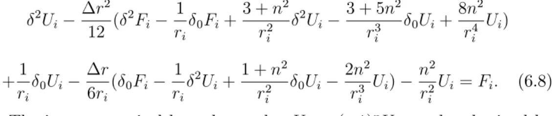
(43) with r = 1=(2M ). Then the outer numerical boundary value UM +2 can be approximated by (6:10). And the inner numerical boundary value U0 is derived as follows. That is, at r = 0:5, 000. U r2 + O( r4 ) 0U = U + 6 00 r2 0 U 1 + n2 0 0 = U + (F + U 6 r r2 0. U2 U0 ^ r2 3F1 + 4F2 = kn + ( 2 r 6 2 r 2 2n U1 ): (0:5)3. F3. 2n2 U ) + O( r4 ): 3 r U2. 2U1 + U0 (1 + n2 ) ^ + kn 0:5 r2 (0:5)2 (6.17). The inner numerical boundary value U0 can be approximated by U0 = (. 6 r 3+2 r 3 2 r2 (1 + n2 ) ^ r )[( )U2 + ( )kn + F1 3 2 r 6 r 3 4 r r 2 + 8n2 r2 F2 + F3 + ( )U1 ]: (6.18) 3 12 3. Table 6.3 shows the maximum errors of this method for three di¤erent solutions of Poisson equation in an annulus with Neumann boundary conditions at r = 1 and 0:5.. 37.

(44) Table 6.3 The Maximum Errors of Di¤erent Solutions to the Poisson Equation with Neumann Boundary @u (0:5; ) = k( ); @u (1; ) = g( ) using N = 64: @r @r 0:5 r 1 M kuk1 Rate u(x; y) = ex+y 16 6.7419E-07 32 4.3156E-08 64 2.7284E-09 128 1.7218E-10 u(x; y) = 3ex+y (x 16 2.5549E-05 32 1.6625E-06 64 1.0601E-07 128 6.6921E-09 x. 3.966 3.983 3.986 x2 )(y. y2) + 5. 3.942 3.971 3.986. y. +e u(x; y) = e1+xy 16 6.5994E-04 32 4.6168E-05 64 3.0672E-06 128 1.9766E-07. 38. 3.837 3.912 3.956.

(45) 7. Conclusions. In this paper, we present a simple and e¢ cient compact fourth-order Poisson solver in cylindrical and spherical coordinates. The solver relies on the truncated Fourier series expansion, where the di¤erential equations of Fourier coe¢ cients have been solved by fourth-order …nite di¤erence discretizations without pole conditions. And two kinds of e¢ cient iterative method, GMRES and Bi-CGSTAB, with di¤erent preconditioners are applied to solve the resulted nonsymmetric systems of Fourier coe¢ cients. In particular, a preconditioner arising from those singular equations have been solved by the second-order …nite di¤erence discrtizations and shown to be the most e¢ cient one. Meanwhile, we can see that the numerical result con…rms the third-order accuracy for the problem on a cylinder. The loss of one order of accuracy can be seen from the discretization near the origin. Therefore, the future research aspect is how to treat the coordinate singularity so that the scheme becomes fully fourth-order accurate.. References [1] Chen, H., Su, Y. & Shizgal, B. D. (2000), A direct spectral collocation Poisson solver in polar and cylindrical coordinates. J. Comput. Phys., 160, 456-469. [2] Lai, M.-C., Lin, W.-W. & Wang, W.-C. (2002), A fast spectral/di¤erence method without pole conditions for Poisson-type equations in cylindrical and spherical geometries. IMA J. Numer. Anal., 22, 537-548. [3] Lai, M.-C. (2002), A simple compact fourth-order Poisson solver on polar geometry. J. Comput. Phys., 182, 337-345. [4] Lai, M.-C. & Wang, W.-C. (2002), Fast direct solvers for Poisson equation on 2D polar and spherical gepmetries. Numer. Meth. Partial Di¤. Eq., 18, 56-68. [5] Quarteroni, A., Sacco, R. & Saleri, F. (2000), Numerical Mathematics (Springer).. 39.

(46) [6] Richard, B. & et al. (1994), Templates for the solution of linear systems:Building blocks for iterative methods (SIAM). [7] Saad, Y. & Schultz, M. (1986), GMRES : A generalized minimal residual algorithm for solving nonsymmetric linear systems. SIAM J. Sci. Statist. Comput., 7, 856-869. [8] Saad, Y. (1996), Iterative Methods for Sparse Linear Systems (PWS Publishing Company). [9] Sonneveld, P. (1989), CGS, a fast Lanczos-type solver for nonsymmetric linear systems. SIAM J. Sci. Statist. Comput., 10, 36-52. [10] Strikwerda, J. C. (1989), Finite Di¤erence schemes and Partial Di¤erential Equations (Wadsworth & Brooks/Cole, Belmonts, CA). [11] Van Der Vorst, H. A. (1992), Bi-CGSTAB : A fast and smoothly converging variant of Bi-CG for the solution of nonsymmetric linear systems. SIAM J. Sci. Statist. Comput., 13, 631-644.. 40.

(47)