以正規轉換為基礎之日夜人物辨識

(1)

國立交通大學

電控工程研究所

碩士論文

以正規轉換為基礎之日夜人物辨識

Canonical Transform Based Day-and-Night Person

Identification

研究生：高仲義

指導教授：張志永

(2)

以正規轉換為基礎之日夜人物辨識

Canonical Transform Based Day-and-Night Person

Identification

學生 : 高仲義 Student : Jhong-

Yi Gao

指導教授 : 張志永 Advisor : Jyh-Yeong Chang

國立交通大學

電機工程學系

碩士論文

A Thesis

Submitted to Department of Electrical Engineering

College of Electrical Engineering

National Chiao-Tung University

in Partial Fulfillment of the Requirements

for the Degree of Master in

Electrical Control Engineering

July 2013

(3)

以正規轉換為基礎之日夜人物辨識

學生: 高仲義指導教授: 張志永博士

國立交通大學電控工程研究所

摘要

人物辨識系統在電腦視覺領域是很熱門的研究與應用目標。在監控系統中，最常見的方式是使用固定式攝影機，對拍攝場景的人物進行人物辨識。本論文實現一套監控系統，此系統是在日夜環境中，分別使用多角度步態辨識系統及人臉辨識系統。本文研究對於使用兩台近紅外線攝影機進行人物辨識，一台近紅外線攝影機設置在遠處，用於擷取不同方向的步態影像，另一台近紅外線攝影機設置在近處，用於擷取人臉正面影像。在人臉辨識系統方面，我們利用近紅外線攝影機擷取人臉影像。人臉擷取的方法是使用 Haar 疊層分類器，這是一種基於特徵運算的演算法，這種演算法比基於逐點的更快速，接著人臉影像經過特徵空間轉換與正規空間轉換後，累積五張上述人臉影像後，藉由多數決的方式，完成人物辨識。在步態辨識系統方面，我們利用近紅外線攝影機擷取步態影像。為了擷取出完整的人體部分，本文使用背景相減法在灰階空間與 HSV 色彩空間建立背景模型，並提升消除影像中陰影部分，使得擷取前景影像能夠更完整，接著步態影像經過特徵空間轉換與標準空間轉換後，累積五張上述步態影像後，藉由多數決的方式，完成人物辨識。

(4)

Canonical Transform Based Day-and-Night Person

Identification

STUDENT:Jhong-Yi Gao ADVISOR: Dr. Jyh-Yeong Chang

Institute of Electrical Control Engineering National Chiao-Tung University

ABSTRACT

Human recognition system is a very popular subject for research and application. Using a camera to recognize human is widely seen in surveillance system.

In this thesis, we implement the surveillance system that can recognize multi-angle human gait and human face of a person in the bright and dark environments. We use two near infrared (NIR) cameras for human recognition. One NIR camera, set in remote location, capture the gait images from different angles. And the other NIR camera, set in the vicinity, capture the face images from the person frontal view.

In human face recognition system, face region of an image is extracted based on Haar cascade classifier, which is a feature-based algorithm and works much faster than the pixel-based algorithm. Then, the face image is transformed to a new space by eigenspace and canonical space transformation for better efficiency and separability. The recognition is finally done in canonical space. Moreover, we gather five consecutive face images from video, and use majority vote to recognition the human.

In human gait recognition system, we build two background models, one in grayscale and one in HSV color space to extract the foreground image correctly. Then

(5)

eigenspace and canonical space transformation for better efficiency and separability. The recognition is done in the canonical space. Finally, we gather five consecutive gait images from video, and use majority vote to recognition the person.

(6)

ACKNOWLEDGEMENTS

I am grateful to my thesis advisor, Professor Jyh-Yeong Chang, who has offered me valuable suggestion in the academic studies. In the preparation of the thesis, he has spent much time reading through each draft and provided me with inspiring advice. Without his patient instruction, insightful criticism and expert guidance, the accomplishment of this thesis would not have been possible.

Finally, I would like to thank my family for their concern, supports and encouragements.

(7)

List of Figures

Fig. 1.1. The flowchart of our human recognition system. ... 2

Fig. 2.1. The HSV color space. ... 7

Fig. 2.2. The framework of background model construction. ... 10

Fig. 2.3. The framework of foreground extraction. ... 14

Fig. 2.4. Histogram of binary foreground image projection in X and Y direction. .. 19

Fig. 2.5. The binary foreground image of extracted foreground region. ... 20

Fig. 2.6. Foreground image after opening and closing operation. ... 20

Fig. 2.7. Rectangle features shown relative to the enclosing detection window. ... 21

Fig. 2.8. Sum of all pixels marked is the integral image intensity at ( , )x y . ... 22

Fig. 2.9. The sum of pixels in rectangle D can be computed as 4+1－(2+3). ... 23

Fig. 3.1. The structure of human recognition by gait or face image sequence. ... 25

Fig. 3.2. The structure of human classification. ... 33

Fig. 4.1. (a) The scene of human gait recognition in bright environments. (b) The scene of human gait recognition in dark environments. (c) The scene of human face recognition in bright environments. (d) The scene of human face recognition in dark environments. ... 35

Fig. 4.2. Example video sequences used in our experiments. (a) and (b) are typical video sequences for gaits of LAB in bright and dark environments. From top to bottom: walking 0°, walking 45°, and walking 315° respectively... 36

Fig. 4.3. Example video sequences used in our experiments. (a) and (b) are typical video sequences for face of LAB in bright and dark environments. From top to bottom: walking 0°, walking 45°, and walking 315° respectively... 37 Fig. 4.4. Eleven video frames depicting person of the CASIA multi-view gait

(10)

Fig. 4.5. Results of foreground detection (a) an image frame in the bright environment, (b) binary image after performing foreground detection in the bright environment, (c) projection of (b) onto X direction, (d) projection of (b) onto Y direction, (e) foreground region segmentation in the bright environment. ... 40 Fig. 4.6. Results of foreground detection (a) an image frame in the dark

environment, (b) binary image after performing foreground detection in the dark environment, (c) projection of (b) onto X direction, (d) projection of (b) onto Y direction, (e) foreground region segmentation in the dark environment. ... 41

(11)

List of Tables

TABLE I THE HUMAN GAIT RECOGNITION RATES AT SPECIFIC WALKING ANGLE IN THE BRIGHT ENVIRONMENT, WITHOUT MAJORITY VOTE

... 43 TABLE II THE HUMAN GAIT RECOGNITION RATES AT SPECIFIC WALKING

ANGLE IN THE BRIGHT ENVIRONMENT, WITH MAJORITY VOTE OF THREE ... 43

TABLE III THE HUMAN GAIT RECOGNITION RATES AT SPECIFIC WALKING ANGLE IN THE BRIGHT ENVIRONMENT, WITH MAJORITY VOTE OF

FIVE ... 44 TABLE IV THE HUMAN GAIT RECOGNITION RATES AT SPECIFIC WALKING

ANGLE IN THE DARK ENVIRONMENT, WITHOUT MAJORITY VOTE 44 TABLE V THE HUMAN GAIT RECOGNITION RATES AT SPECIFIC WALKING

ANGLE IN THE DARK ENVIRONMENT, WITH MAJORITY VOTE OF THREE ... 45

TABLE VI THE HUMAN GAIT RECOGNITION RATES AT SPECIFIC WALKING ANGLE IN THE DARK ENVIRONMENT, WITH MAJORITY VOTE OF

FIVE ... 45 TABLE VII THE RECOGNITION RATES OF WALKING VIDEOS IN THE BRIGHT

ENVIRONMENT, WITHOUT MAJORITY VOTE ... 47 TABLE VIII THE RECOGNITION RATES OF WALKING VIDEOS IN THE BRIGHT

ENVIRONMENT, WITH MAJORITY VOTE OF THREE ... 47 TABLE IX THE RECOGNITION RATES OF WALKING VIDEOS IN THE BRIGHT

(12)

ENVIRONMENT, WITHOUT MAJORITY VOTE ... 48 TABLE XI THE RECOGNITION RATES OF WALKING VIDEOS IN THE DARK

ENVIRONMENT, WITH MAJORITY VOTE OF THREE ... 48 TABLE XII THE RECOGNITION RATES OF WALKING VIDEOS IN THE DARK

ENVIRONMENT, WITH MAJORITY VOTE OF FIVE ... 48 TABLE XIII THE HUMAN RECOGNITION RATES AT SPECIFIC VIEWING ANGLE

IN THE CASIA DATABASE, WITHOUT MAJORITY VOTE ... 50 TABLE XIV THE HUMAN RECOGNITION RATES AT SPECIFIC VIEWING ANGLE

IN THE CASIA DATABASE, WITH MAJORITY VOTE OF THREE ... 51 TABLE XV THE HUMAN RECOGNITION RATES AT SPECIFIC VIEWING ANGLE IN

THE CASIA DATABASE, WITH MAJORITY VOTE OF FIVE ... 52 TABLE XVI THE RECOGNITION RATES AT ALL VIEWING ANGLES IN THE CASIA

DATABASE, WITHOUT MAJORITY VOTE ... 53 TABLE XVII THE RECOGNITION RATES AT ALL VIEWING ANGLES IN THE

CASIA DATABASE, WITH MAJORITY VOTE OF THREE ... 54 TABLE XVIII THE RECOGNITION RATES AT ALL VIEWING ANGLES IN THE

CASIA DATABASE, WITH MAJORITY VOTE OF FIVE ... 54 TABLE XIX THE RECOGNITION RATES OF HUMAN FACE VIDEOS IN THE

BRIGHT ENVIRONMENT, WITHOUT MAJORITY VOTE ... 56 TABLE XX THE RECOGNITION RATES OF HUMAN FACE VIDEOS IN THE

BRIGHT ENVIRONMENT, WITH MAJORITY VOTE OF THREE ... 57 TABLE XXI THE RECOGNITION RATES OF HUMAN FACE VIDEOS IN THE

BRIGHT ENVIRONMENT, WITH MAJORITY VOTE OF FIVE ... 58 TABLE XXII THE RECOGNITION RATES OF HUMAN FACE VIDEOS IN THE DARK

(13)

DARK ENVIRONMENT, WITH MAJORITY VOTE OF THREE ... 60 TABLE XXIV THE RECOGNITION RATES OF HUMAN FACE VIDEOS IN THE

(14)

Chapter 1 Introduction

1.1 Motivation

Human recognition plays an important role in applications such as surveillance systems, home nursing care system and security applications. Most of the security service firm is provided by professional people, such as security guard. However, the service cost is very expensive and the security guard cannot watch camera video in 24 hours. Therefore, the automatic surveillance system becomes a popular research area in recent years. For example, an automatic system will trigger an alarm condition when the automated surveillance system detects and recognizes suspicious human.

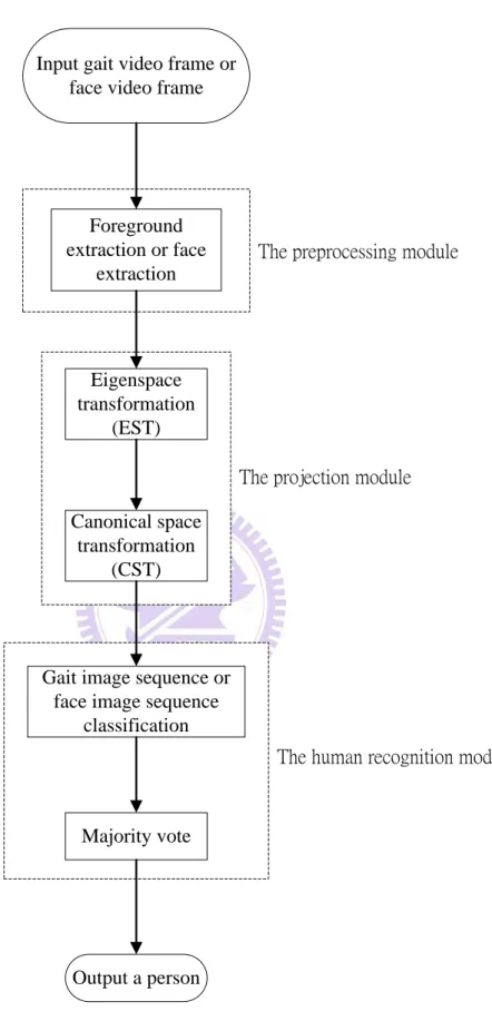
In this thesis, we implement the day-and-night (bright and dark) surveillance system that separately using multi-angle human gait and human face recognition of a person in an In-door Environment. We use two cameras for human recognition. One camera being used to capture the gait image from different angle is set in a remote location. And the other camera being used to capture the face image from the person frontal view is set in the vicinity. Fig 1.1 is illustrated our system flowchart. Our system can be separated into three components. The first component is video frame preprocessing which contain foreground subject extraction and human face extraction. The second component is the transformation of human gait image or human face image in a space smaller and easier for human recognition. The third component is the human recognition of an image frame using majority vote.

(15)

Input gait video frame or face video frame

Foreground extraction or face extraction Eigenspace transformation (EST) Canonical space transformation (CST)

Gait image sequence or face image sequence

classification

Majority vote

Output a person

The preprocessing module

The projection module

The human recognition module

(16)

1.2 Video Frame Preprocessing for Human Recognition

The first step of human gait recognition system is foreground subject extraction. We have to construct a background model for foreground subject extraction. Background subtraction is widely used for detecting moving objects from image frames of fixed cameras. The rationale of this approach is to detect the moving objects by the difference between the current image frame and a reference image frame, often called the “background model.” There are many well-known methods to build background models. A review is given in [1] where many different approaches were proposed in recent years. In our human gait recognition system, we construct two background models for more correct foreground subject extraction; one is based on grayscale value, and the other is based on HSV color space. Basically, the background image is a representation of the static scene. We have to update the background model after the subject enters the scene. After the subject leaves the scene, the background model will also be updated accordingly.

After construct two background models, we can extract foreground subject from video frames by subtracting each pixel value of background model from that current image frame. Then, the resulting image is converted to a binary image by setting a threshold. The binary image contains foreground subject and shadow. Therefore, we need to remove the shadow by using a shadow filter. Then, we can set a threshold in the histogram of the binary image to extract a rectangle image, which is the most resemble shape of a person. When we want to remove shadow pixels, some foreground pixel will be lost and this makes the foreground image broken. Therefore, we will repair the rectangle image by using opening and closing operations. Finally, the rectangle image is resized to the specified resolution for normalization.

(17)

purpose of face detection is to localize and extract the face region from the scene with human. We use Haar cascade classifier, proposed by Viola et al. [2], from OpenCV package [3] to detect the face regions.

1.3 Video Frame Human Recognition Procedure

In gait video or face video, the dimensions of gait image or face image are often extremely large, and these images usually contain great deals of redundancies. Hence, some space transformations are introduced to reduce redundancy of an image by reducing the size of the image. The first step of redundancy reduction often transforms an image from spatiotemporal space to another data space. The transformation can use fewer dimensions to approximate the original image. There are many well-known transformation methods for human recognition, for example, wavelet transformation, Fourier transformation, Locally Linear Embedding (LLE), Multi Dimension Scaling (MDS), Principal Component Analysis (PCA), eigenspace transformation (EST), and so on. Our transformation method combines eigenspace transformation and canonical space transformation which are described as follows.

Eigenspace transformation (EST), which uses Principal Component Analysis (PCA) for dimensionality reduction, has been demonstrated to be a potent scheme used below: automatic face recognition proposed in[4], [5]; gait analysis proposed in [6]; and action recognition proposed in [7]. The subsequent transformation, Canonical space transformation (CST) based on Canonical Analysis, is used to reduce data dimensionality and to optimize the class separability and improve the classification performance. Unfortunately, CST approach needs high computation efforts when the image is large. Therefore, we combine EST and CST in order to improve the

(18)

be projected from a high-dimensional spatiotemporal space to a single point in a low-dimensional canonical space.

Due to the above classification we used nearest neighbor concept to do the human recognition in the video. There could be misclassifications in some frames; we have adopted the majority vote to conduct the human recognition, to overcome this problem.

1.4 Thesis Outline

The thesis is organized as follows. In Chapter 2, we introduce video frame preprocessing for human gait recognition and human face recognition. In Chapter 3, we describe our human recognition system that includes “eigenspace transform,” “canonical transform,” “human recognition,” and “majority vote.” In Chapter 4, the experiment results of our human recognition systems are shown. At last, we conclude this thesis with a discussion in Chapter 5.

(19)

Chapter 2 Video Frame Preprocessing for Human

Recognition

In this chapter, we describe background model construction and foreground extraction in grayscale and the HSV color space. We also briefly introduce the basic concepts of HSV color space which transforms the coordinate system in RGB color space to HSV color space. Finally, we introduce face detection method whose the principle is based on object detection technology proposed by Viola et al. [2].

2.1 The HSV color space

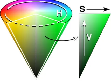
The HSV color space stands for hue, saturation, and value, also called HSB (B for brightness), which corresponds closely to the human perception of color. Fig. 2.1 illustrates the HSV color space whose shape is like a cone. From this figure, the hue is represented by the angle of each color in the cone relative to the 0° line, which is traditionally corresponded to be red. The saturation is representing as the distance from the center of the circle. Highly saturation color is on the outer edge of the cone, whereas gray tones (which have no saturation) are at the very center. The value is determined by the colors vertical position in the cone. At the point end of the cone, there is no brightness, so all colors are blacks. At the fat end of the cone are the brightness colors.

(20)

Fig. 2.1. The HSV color space.

The formula of RGB transfers to HSV is given by

0 , if 60 0 , if and 60 360 , if and 60 120 , if 60 240 , if max min G B max R G B max min G B max R G B H max min B R max G max min R G max B max min   ° =    ₋ °× + ° = ≥  − − °× + ° = < = − − °× + ° = − − °× + ° = − 0, if 0 1 , otherwise max S _max _min _min

max max V max               =   =_ ₋ = −  = (2.1)

(21)

where max=max

(

R G B, ,

)

and min=min

(

R G B, ,

)

.

The hue parameter is the value which represents color information without brightness. Therefore, the hue is not affected by change of the illumination brightness and direction. Although the hue is the most useful attribute, there are three problems in using hue attribute for color segmentation: 1) the hue is unstable when the saturation is extremely small. 2) The hue is meaningless when the intensity value is extremely small. 3) The saturation is meaningless when the intensity value is extremely small [8]. Accordingly, Ohba et al. [9] use three criteria (intensity value, saturation, and hue) to obtain the hue value reliably.

 Intensity Threshold Value:

If V < , then V_t H =0, where V, V , and H are an intensity value, the _t

intensity threshold value, and a hue value, respectively. Using this equation, the measured color close to dark is discarded. Then, the hue value is set to a predetermined value, i.e., 0.

 Saturation Threshold Value:

If S< , then S_t H =0, where S, S , and H are a saturation value, the _t

saturation threshold value, and a hue value, respectively. Using this equation, measured color close to gray is discarded in the image.

 Hue Threshold Value:

If H < ∆ or P_t H−2π < ∆ , then P_t H =0, where H and ∆ are a hue P_t

value, and the phase threshold value, respectively. The range of hue value is from 0 to 2π, and it has discontinuity at 0 and 2π. We use the phase threshold value

t

P

(22)

2.2 Background Model Construction and Foreground Extraction

The first step of human gait recognition system is foreground extraction. We have to construct the background model for foreground extraction. There are many well-known methods to build background models. W is such a typical example 4 with some modifications [10]. It records the maximum grayscale value and the minimum grayscale value and the maximum inter-frame absolute difference of each pixel in the background video frames. Then each foreground image frame subtracts the maximum and minimum intensity value of each pixel. If the pixel’s absolute value of the subtraction operation is larger than the maximum inter-frame difference, the pixel is classified as a foreground pixel. W admits some rules make the 4 background model be adaptive to varying environment.

2.2.1 Background Model Construction

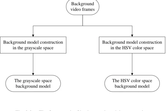
If we only construct the luminance background model for foreground extraction, it cannot detect reliably those foreground pixel whose luminance component close to background pixel. In order to solve this problem, we construct another background model in HSV color space. The HSV color space corresponds closely to the human perception of color. We can have the luminance information and the chromatic information simultaneously. The hue is unreliable in some condition, so we use the three criteria (intensity value, saturation, and hue) described in sections 2.1 to obtain the hue value reliably. Fig. 2.2 shows the framework of background model construction.

(23)

Background video frames

Background model construction in the grayscale space

Background model construction in the HSV color space

The grayscale space background model

The HSV color space background model

Fig. 2.2. The framework of background model construction.

A. Grayscale Value Background Model

The grayscale value background scene is modeled by representing each pixel by three values: the maximum grayscale value n x y and the minimum grayscale

(

,

)

value m x y and the maximum inter-frame difference

( )

, d x y of each pixel in

(

,

)

the background video frames. Because these three values are statistical, we need a background video without any moving foreground objects for background model training. Let I be a background image frame sequence and contains N consecutive image frames. I x y be the grayscale value of a pixel location _i

(

,

)

(

x y in the i-th ,

)

background image frame of I. The grayscale value background model for a pixel location

(

x y , ,

)

_n x y

(

, ,

) (

m x y, , ,

) (

d x y

)

_{ , is obtained by}

(24)

(

)

(

)

(

)

(

)

{

}

(

)

{

}

(

)

(

)

{

1

}

max , , , min , , 1, 2, , , _max _{, ,} i i i i i i i I x y n x y m x y I x y i N d x y _{I x y} _I _{x y} −    _{ } _  _{ } _ = =  _{ } _  _{ } _   __ − __  (2.2)

B. HSV Color Space Background Model

Along similar line of reasoning of above, we construct another background model in each dimension of HSV (hue, saturation and value) space [11]. Then, we record the

maximum value

(

)

S

(

)

(

)

, , , , ,

H V

n x y n x y n x y

 

  and the minimum value

(

)

(

)

(

)

(

S

)

, , , , , H V m x y m x y m x y  

  and the inter-frame ratio in the brightness

information and the inter-frame different in the chromatic information. Similarly, we use the same background video without any moving foreground objects for background model training. Let I be a background image frame sequence and contains

N consecutive background image frames. I_iH

(

x y is the hue value of a pixel ,

)

location

(

x y in the i-th background image frame of I. ,

)

I_iS

(

x y is the saturation ,

)

value of a pixel location

(

x y in the i-th background image frame of I. ,

)

I_iV

(

x y ,

)

is the brightness value of a pixel location

(

x y in the i-th background image frame ,

)

of I. The HSV color space background model of a pixel is obtained by

(

)

(

)

(

)

(

)

{

}

(

)

{

}

(

)

(

)

{

}

max , , , min , , 1, 2, , , H H i i H H i i H I x y n x y m x y I x y i N d x y    _{ } _  _{ } _ = =  _{ } _  _{ } _     −  (2.3)

(25)

(

)

(

)

(

)

(

)

{

}

(

)

{

}

(

)

(

)

{

1

}

max , , , min , , 1, 2, , , _max _{, ,} S S i i S S i i S S S i i i I x y n x y m x y I x y i N d x y _I _{x y} _I _{x y} −    _{ } _  _{ } _ = =  _{ } _  _{ } _     __ − __  (2.4)

(

)

(

)

(

)

(

)

{

}

(

)

{

}

(

)

(

)

{

}

(

)

(

)

(

)

{

}

1 1 max , min , , if , / , 1 max , / , , , , _max _, min V i i V V V i i i i V V V i i i V V _V i i i i I x y I x y I x y I x y I x y I x y n x y m x y d x y _I _{x y} I − −       _≥       _ _   =        

(

)

{

}

(

)

(

)

{

1

}

, , otherwise max , / , 1, 2, , V V V i i i x y I x y I x y i N −                        =  (2.5)

2.2.2 Background Update

The background model cannot be expected to stay the same for a long time. If the facilities in room are moved, they will be detected as foreground pixels of human and the human recognition will be misclassified. Therefore, we have to adopt a scheme that can update the background models in order to avoid above situation. The background models will be updated if the real-time video does not vary for a long time and there is nobody in the scene. By Eq. (2.6), we can calculate how many times the binary value remain unchanged.

(26)

(

)

(

)

(

)

(

)

(

)

1 , 1, if , , , , , otherwise t t foreground foreground update x y I x y I x y update x y update x y −  + =  =    (2.6)

where It_foreground

(

x y is the grayscale value of a pixel location ,

)

(

x y in the binary ,

)

image. The update x y value is a record of how many times

(

,

)

It_foreground

(

x y ,

)

remains unchanged. When update x y

(

,

)

exceeds a threshold, the pixel

(

x y will ,

)

be included in the background model.

2.2.3 Foreground Extraction

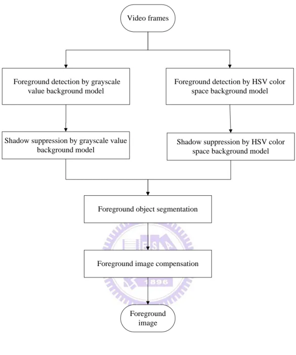
The framework of foreground extraction is composed of four steps. The first step is foreground detection in the grayscale value and the HSV color space background models. The second step is the shadow suppression in the grayscale value and the HSV color space background models. The third step is the foreground object segmentation. And the final step is the foreground image compensation to recover the foreground pixels those are wrongly classified to the background. Fig. 2.3 shows the framework of foreground extraction.

(27)

Video frames

Foreground detection by grayscale value background model

Foreground detection by HSV color space background model

Shadow suppression by grayscale value background model

Foreground object segmentation

Foreground image compensation

Foreground image

Shadow suppression by HSV color space background model

Fig. 2.3. The framework of foreground extraction.

A. Foreground Detection

The foreground objects can be detected from the background in each frame of the video sequence. Each pixel of the video frame is classified to either a foreground or a background pixel using the background model. First, we use the maximum grayscale

(28)

value n x y and the minimum grayscale value

(

,

)

m x y and the maximum

( )

, inter-frame difference d x y of the grayscale value background model to detect

(

,

)

the foreground pixel by

(

)

(

)

(

)

(

)

(

)

0 background, if , y , or , y , , 1 foreground, otherwise. gray gray i gray gray gray i gray fg I x n x y k d I x m x y k d I x y µ µ  − <   ₋ _< =     (2.7)

where I x y is the grayscale value of a pixel location _i

(

,

)

(

x y in the i-th video ,

)

frame, I_fg

(

x y is the gray level of a pixel in the foreground binary image, d,

)

_µ is the median of all dgray

(

x y , and ,

)

k_gray is a threshold. Threshold k_gray is determined by experiments according to different environments.

On the other hand, we use the maximum value nV

(

x y and the minimum value ,

)

( )

,

V

m x y and the maximum inter-frame ratio dV

(

x y of the HSV color space ,

)

background model to detect the foreground pixel by

(

)

(

)

(

)

(

)

(

)

(

)

(

)

0 background, if , y / , , or , y / , , , V V V i V V V V HSV i V fg I x n x y k d x y I x m x y k d x y I x y  <  <  =    (2.8)

(29)

where I_iV

(

x, y

)

is the intensity value of a pixel location

(

x y in the i-th video ,

)

frame, IHSV_foreground

(

x y is the gray level of a pixel in binary image, and threshold ,

)

k V

is determined by light as of the scene. Threshold k will be reduced for in-sufficient _V

light condition and increased otherwise.

B. Shadow Suppression

The shadows of the foreground object are easily detected to foreground pixels in normal conditions. The situation causes foreground object merging and foreground object shape distortion in binary image. Therefore, we need to remove the shadow by using the shadow filter. We assume that the observed intensity of shadow pixels is directly proportional to incident light. Consequently, shadowed pixels are scaled versions (darker) of corresponding pixels in the background model [12].

First, we construct the shadow filter in the grayscale value. Let B x y be the

(

,

)

background image formed by temporal median filtering, and I x y be an image of

(

,

)

the video sequence. For each pixel

(

x y belonging to the foreground, consider a ,

)

3 3× template T_xy such that Txy

(

m n, ,

) (

=I x m y+ +n

)

, where -1≤m≤1, -1≤ ≤n 1

(i.e. T corresponds to a neighborhood of pixel _xy

(

x y ). Then, the NCC between ,

)

templates T and background image B at pixel _xy

(

x y is given by ,

)

(

,

)

₍

(

,

₎

)

, xy B T ER x y NCC x y E x y E = (2.9)

(30)

where

(

)

(

) (

)

(

)

(

)

(

)

1 1 1 1 1 1 2 1 1 1 1 2 1 1 , , , , , , , , . xy xy m n B m n T xy m n ER x y B x m y n T m n E x y B x m y n E T m n =− =− =− =− =− =− = + + = + + =

∑ ∑

(2.10)

For a pixel

(

x y in a shadow region, the NCC in a neighboring region ,

)

T should _xy

be large (close to one), and the energy xy

T

E of this region should be lower than lower

than the energy E of the corresponding region in the background image. Therefore, _B

we get

(

)

(

)

(

)

shadow, if , and , , foreground, otherwise ncc B gray NCC x y L E E x y S x y ≥ <   =    xy T (2.11)

where Sgray

(

x y is the shadow mask to class the pixel in grayscale domain , and ,

)

ncc

L is a fixed threshold. If L_ncc is low, several foreground pixels corresponding to moving objects may be misclassified as shadow pixels. Otherwise, selecting a larger value of L_ncc, then the shadow pixels may not be detected.

(31)

but lower brightness than the background model. Therefore, we construct another shadow filter in the HSV color space is intuitively designed as follows

(

)

(

)

(

)

(

)

(

)

(

)

(

)

(

)

(

)

shadow, if , / , 1 and , , , , and , , , foreground, otherwise V V i H H H i H HSV S S S i S I x y m x y I x y n x y k d x y S x y I x y n x y k d x y  <  − <  =  − <    (2.12)

where I_iH

(

x y, ,

)

I_iS

(

x y, ,

)

and IV_i

(

x y are respectively the HSV channel of a ,

)

pixel location

(

x y in the i-th video frame, and ,

)

SHSV

(

x y is the shadow mask to ,

)

class the pixel in HSV domain. Values k and _S k are selected threshold values _H

used to measure the similarities of the hue and the saturation between the background image and the current observed image.

In order to reduce the impact caused by shadow and noise on the foreground object, we calculate the union of Sgray

(

x y and ,

)

SHSV

(

x y . The reason why we ,

)

choose the union operator is that the union can increase the foreground with less noise. Finally, the binary image is obtained by

(

, , ,

)

gray

(

)

HSV

(

)

fg

I x y =S x y ∨S x y (2.13)

C. Foreground Object Segmentation

(32)

region of foreground object to minimize the image size. Foreground region extraction can be accomplished by simply introducing a threshold on the histograms in the X and Y directions. Fig. 2.4 shows an example of foreground region extraction. From this figure, we use the binary image and project it into the X and Y directions. The interested foreground section has higher counts in the histogram. We obtain the boundary coordinates x x₁, ₂ of X axis and y y₁, ₂ of Y axis from the projection histogram. We can use these boundary coordinates as four corners of a rectangle to extract foreground region and the size of this rectangle is adjusted to 64 48× _for

(33)

Fig. 2.5. The binary foreground image of extracted foreground region.

D. Foreground Image Compensation

Detecting all foreground pixels and removing all shadows simultaneously are difficult. When we want to remove shadow pixels, some foreground pixels will be lost and this makes the foreground image be broken. Therefore, we will repair the foreground image by opening and closing operations [13]. Fig. 2.6 (a) shows all foreground pixels after shadow removal, and Fig. 2.6 (b) shows the result after applying the opening and closing operations.

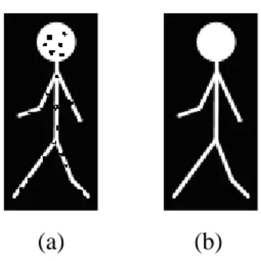
(a) (b) Fig. 2.6. (a) Foreground image. (b) Foreground image after opening and closing of (a).

(34)

2.3 Face Extraction

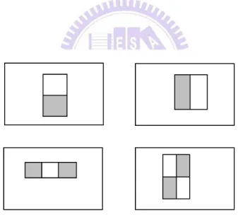
The first step of human face recognition system is face extraction. We use Haar cascade classifier, proposed by Viola et al. [2], from OpenCV package [3] to detect the face regions. The classifier is based on the value of simple features. The feature-based system operates much faster than the pixel-based system. The feature-based system utilizes three kinds of features. The two-rectangle feature,

three-rectangle feature and four-rectangle feature to classify facial region and not

facial region (see Fig. 2.7). The sum of the pixels which lie within the white rectangles is subtracted from the one within the gray rectangles, and then the value is considered as a feature.

Fig. 2.7. Rectangle features shown relative to the enclosing detection window.

The cost of calculation of rectangle features can be reduced by using the integral image. The integral image intensity at location ( , )x y is the sum of the pixels above

(35)

(

)

(

)

, , , x x y y ii x y i x y ′≤ ′≤ ′ ′ =

∑

(2.14)

where ii x y is the integral image and

(

,

)

i x y

(

′ ′ is the original image (see Fig. ,

)

2.8)

Fig. 2.8. Sum of all pixels marked is the integral image intensity at ( , )x y .

The integral image can be computed in just one pass over the original image by using the following pair of recurrences:

(

,

) (

, 1

) (

,

)

s x y =s x y− +i x y (2.15)

(

,

)

(

1, ,

) (

)

ii x y =ii x− y +s x y (2.16)

(36)

rectangular sum can be computed in four array references (see Fig. 2.9). The sum of pixels in rectangle A is the integral image intensity at location 1. The sum of A+B is at location 2, A+C is at location 3 and A+B+C+D is at location 4. Therefore, the sum of pixels in rectangle D can be computed as 4+1－(2+3).

Fig. 2.9. The sum of pixels in rectangle D can be computed as 4+1－(2+3).

A variant of AdaBoost is used to select the features and train the classifier. The objective of the AdaBoost algorithm is to form a stronger classifier by combining a collection of weak classification functions. If the correct rate of a weak classifier is above 50%, it is a good weak classification function. Finally, the Haar cascade classifier is built by stringing strong classifiers for detecting face region more accurately.

(37)

Chapter 3 Video Frame Human Recognition

Procedure

3.1 Human Representation

In video and image processing, the dimensions of image data are often very large. Each image data is suggested to transform from high-dimensional space into low-dimensional space to obtain a small set of composite feature for human recognition. There are many well-known transformation methods for human recognition, for example, wavelet transformation, Fourier transformation, Locally Linear Embedding (LLE), Multi Dimension Scaling (MDS), Principal Component Analysis (PCA), eigenspace transformation (EST), and so on. However, PCA based on the global covariance matrix of the full set of image data is designed for efficient data representation, not sensitive to the class structure existent in the image data. In order to enhance the discriminatory power of several image features, Etemad and Chellappa [14] use linear discriminant analysis (LDA), also called Canonical Analysis [6], which can be used to optimize the class separability of different image classes and improve the classification performance. To this end, the features are obtained by maximizing between-class and minimizing within-class variations. Unfortunately, this approach has high computation cost when applying to large images. It was only tested with small images. Here we call this approach canonical space transformation (CST). Combining EST based on PCA with CST based on CA, our approach reduces the data dimensionality and optimizes the class separability of different gait sequences.

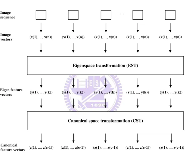
Images in high-dimensional space are first converted into low-dimensional eigenspace using EST. The obtained vector thus is further transformed to a smaller canonical space using CST. Human recognition is accomplished in the canonical

(38)

space. Fig. 3.1 shows the processing steps that generate feature vectors by eigenspace transformation and canonical space transformation each image is converted to an one-dimension canonical vector. Apparently, the reduced dimensionality results in concomitant decrease in computation cost.

Canonical space transformation (CST) Eigenspace transformation (EST)

Image sequence Image vectors (x(1), ..., x(n)) (x(1), ..., x(n)) (x(1), ..., x(n)) (x(1), ..., x(n)) (x(1), ..., x(n)) Eigen feature vectors Canonical feature vectors

(y(1), ..., y(k)) (y(1), ..., y(k)) (y(1), ..., y(k)) (y(1), ..., y(k)) (y(1), ..., y(k))

(z(1), ..., z(c-1)) (z(1), ..., z(c-1)) (z(1), ..., z(c-1)) (z(1), ..., z(c-1)) (z(1), ..., z(c-1))

…

Fig. 3.1. The structure of human recognition by gait or face image sequence.

Assume that there are c classes of person to be learned. Each class is represented by a specific viewing angle gait image sequences or face image sequences of a person,

(39)

j-th image in the i-th class person, and N_i is the number of images of the i-th class

image sequence acquired. The total number of training image data in training set is

1 2

T c

N =N +N + + N . The training set can be represented as

1

1, 1, , 1, N , 2, 1, , c N, _c

 ′ ′ ′ ′ 

x  x x  x  (3.1)

where each x′_{i j}_, is an image data with n pixels.

First, the intensity of each image data is normalized by

, , , i j i j i j ′ = ′ x x x (3.2)

Then, the mean pixel value for the training set is obtained by

, 1 1 1 c Ni i j i j T N = = =

∑∑

x m x (3.3)

By subtracting the mean m_x from each image data, the training set can be rewritten

as a n N× _T matrix X, with each image data x_{i j}′_, forms a column of X, then

1

1, 1 , , 1, N , , c, Nc

 

=_ − _x − _x − _x_

(40)

3.1.1 Eigenspace Transformation (EST)

EST is used to reduce the dimensionality of an input space by mapping the image data from high-dimensional space into low-dimensional space while maintaining the minimum mean-square error to avoid information loss. EST uses the eigenvalues and eigenvectors generated by the image data covariance matrix to rotate the original image data coordinates along the directions of maximum variance sequentially. We can compute image data covariance matrix R, then

T

=

R XX (3.5)

where R is a square, symmetric n n× matrix.

If the rank of the matrix R is K, then the K nonzero eigenvalues of R,

1 2

λ , λ , ,  λK, and associated eigenvectors e1, , , e2  eK satisfy the fundamental

relationship

λ_ιe_i =Re_i, i=1, 2, , K (3.6)

In order to solve Eq. (3.6), we need to compute the eigenvalues and eigenvectors of the n n× matrix R. But the dimensionality of R is the image data size, it is often

extremely large. Based on singular value decomposition, we can obtain the eigenvalues and eigenvectors by computing another image data covariance matrix R instead, that is

T

(41)

where R is a square, symmetric N_T×N_T matrix which is much smaller than n n×

of R.

If the rank of the matrix R is K, then the K nonzero eigenvalues of R ,

1 2

λ , λ , ,    λK, and corresponding eigenvectors e1, , , e2  eK which are related to

those in R by 1 2 λ λ , 1, 2, , λ i i i i i i K −  =  ₌   = e Xe    (3.8)

These K eigenvectors are used as an orthogonal basis to span a new vector space. Each image data can be projected to a point in this K-dimensional space. Based on the theory of PCA, each image data can be approximated by taking only the k largest eigenvalues λ₁ ≥ λ₂ ≥≥ λ_k , ,k≤K and their corresponding eigenvectors

1, , , 2 k

e e  e . This partial set of k eigenvectors spans an eigenspace in which y_{i j}_,

are the data points that are the projections of the original image data x_{i j}_, by the equation

[

]

T

, 1, 2, , , , 1, 2, , and 1, 2, , c

i j = k i j i= c j= N

y e e  e x   (3.9)

This matrix

[

e₁, , , e₂  e_k

]

T is called the eigenspace transformation matrix. After

this transformation, each original image data x_{i j}_, can be approximated by the linear combination of these k eigenvectors and y_{i j}_, is a one-dimensional vector with k

(42)

3.1.2 Canonical Space Transformation (CST)

According to the theory of canonical analysis [15], we suppose that

{

Φ Φ1, , , 2  Φc

}

represents the classes of transformed vectors by eigenspace

transformation and y_{i j}_, is the j-th vector in class i. The mean vector of entire set is obtained by , 1 1 1 c Ni i j i j T N = = =

∑∑

y m y (3.10)

and the mean vector of the i-th class can be represented by

, , 1 i j i i j i N ∈Φ =

∑

y m_i y (3.11)

Let S denote the between-class scatter matrix and _b S denote the within-class _w

scatter matrix, then

(

)(

)

(

)(

)

, 1 , , 1 1 1 i j i c b i i y i y i T c w i j i i j i i T N N N Τ = Τ = ∈Φ = − − = − −

∑

∑ ∑

y S m m m m S y m y m

(43)

and minimize S simultaneously, which is known as the generalized Fisher linear_w

discriminant function and obtained by

( )

b w Τ Τ = W S W J W W S W (3.12)

The ratio of variances in the new space is maximized by the selection of feature transformation W if 0 ∂ ₌ ∂ J W (3.13)

We suppose the W* is the optimal solution where the column vector w*_i is a

generalized eigenvector corresponding to the i-th largest eigenvalues λ_i. Based on the theory of canonical analysis [15], we can solve Eq. (3.13) as follows

* *

b i = λi w i

S w S w (3.14)

After Eq. (3.14) is solved, we will obtain c−1 nonzero eigenvalues and associated eigenvectors v v₁, ₂,,v_c₋₁ that create another orthogonal basis and span a

(

c− -dimensional canonical space. By using these bases, each data point in 1

)

eigenspace can be transformed to another data point in canonical space by

[

]

, 1, 2, , 1 , i j c i j Τ − = z v v  v y (3.15)

(44)

where z represents the new data point. This orthogonal basis _{i j}_,

[

v v₁, ₂,,v_c₋₁

]

Τ is

called the canonical space transformation matrix.

By merging Eq. (3.9) and Eq. (3.15), each image data can be transformed into a new data point in the

(

c− -dimensional space by 1

)

, , i j = i j z Hx (3.16) , 1 1 Ni i i j j i N

∑

= C = z (3.17)

where H=

[

v₁, , , v₂  v_c₋₁

] [

Τ e₁, , , e₂  e_k

]

Τ and C is the centroid of class i. _i

3.2 Human Recognition

3.2.1 Person Recognition by Gait Image Classification in a Long

Distance Setting

When a video stream is inputted for human gait recognition, we extract image frames from the video first. Then we use background model of Section 2.2 to extract foreground subject from the scene. The foreground object is a binary image, also called as the gait template which is converted to low-dimensional eigenspace using EST in high-dimensional image space. The obtained vector thus is further projected to a smaller canonical space using CST. As described in Section 3.1, each gait template is transformed to a (c － 1)-dimensional vector by EST and CST methods. To recognize a gait template from the video frame sequence in the canonical space, the

(45)

the gait class center “G ,” as given by _i

arg min i , 1, 2, , g i

j= g−G i=  c (3.18)

where c is number of gait class and j is the result of person recognition. _g

3.2.2 Person Recognition by Face Image Classification in a Short

Distance Setting

When a video stream is inputted for human face recognition, we extract image frames from the video first. Then we use face detection of Section 2.3 to extract human face from the scene. The human face is a grayscale image, also called as the face template which is converted to low-dimensional eigenspace using EST in high-dimensional image space. The obtained vector thus is further projected to a smaller canonical space using CST. As described in Section 3.1, each face template is transformed to a (c－1)-dimensional vector by EST and CST methods. To recognize a face template from the video frame sequence in the canonical space, the minimal

Euclidean distance to each centroid is used. The recognition class is assigned to the

class which assumes the minimal distance between a test face template “f,” and the face class center “F ,” as given by _i

arg min i , 1, 2, , f i

j= f −F i=  c (3.19)

(46)

3.2.3 Majority Vote

Due to the above classification which use each frame to do the human recognition in the video, there may have misclassifications in some frames. To overcome this problem, we have adopted the majority vote to conduct the human recognition. Fig. 3.2 shows the structure of the human classification.

Eigenspace and Canonical space transformation

Image sequence Image vectors (x(1), ..., x(n)) (x(1), ..., x(n)) (x(1), ..., x(n)) (x(1), ..., x(n)) (x(1), ..., x(n)) Canonical feature vectors (z(1), ..., z(c-1)) (z(1), ..., z(c-1)) (z(1), ..., z(c-1)) (z(1), ..., z(c-1)) (z(1), ..., z(c-1)) …… (x(1), ..., x(n)) (z(1), ..., z(c-1)) Time

Calculate the nearest cluster center

Majority vote

Human

(47)

Chapter 4 Experimental Results

In our experiment, we tested our system on videos taken by near infrared (NIR) camera (KMT-1651N with 12 lighting led cells) in our laboratory at the 5th Engineering Building in NCTU campus. We use two cameras for human recognition from facial and walking videos. The first is far NIR camera with a lens focus 4.3mm is set up at the location far from the object about 6 meters, and the second is near NIR camera with a lens focus 6.0mm is setup at the location far from the object about 2.5 meters. These cameras have a frame rate of 30 frames per second and image resolution is 320 240× pixels. The background of the experiment environment is in real life and the illumination of the environment is 398 Lux in the bright environment and 0.26 Lux in the dark environment, respectively. Fig. 4.1(a) shows the scene of human recognition for gait videos in the bright environment. Fig. 4.1(b) shows the scene of human recognition for gait videos in the dark environment. Fig. 4.1(c) shows the scene of human recognition for face videos in the bright environment. Fig. 4.1(d) shows the scene of human recognition for face videos in the dark environment.

Our LAB gait multi-angle database consists of 32 image sequences consisting of eight persons walking in the bright and dark environments. Each person was done four times producing four sequences at three different walking angles (0°, 45°, and 315 °) with respect to the person frontal view in a clockwise sense. Thus, it contains a total of 4 8 3× × =96 walking video sequences for human recognition. Fig. 4.2 shows the examples video sequence form our LAB gait multi-angle databases. On the other hand, our LAB face database consists of 36 video sequences consisting of nine persons in the bright and dark environments. Moreover, each person has four face video sequences in the bright and dark environments. Fig. 4.3 shows the examples video

(48)

Furthermore, we also tested our system on CASIA database [16] which contains multi-view gait sequences. The CASIA database [17] consists of 288 image sequences depicting 48 persons. Each person is depicted in six sequences at 11 different viewing angles (0°, 18°, 36°, 54°, 72°, 90°, 108°, 126°, 144°, 162°, and 180°) with respect to the person frontal view in a counterclockwise manner. Thus, it contains a total of

6 48 11× × =3168 gait sequences. Binary body image masks are provided in the CASIA database. Eleven video frames depicting person in the CASIA database from each viewing angle are illustrated in Fig. 4.4.

(a) (b)

(c) (d)

Fig. 4.1. (a) The scene of human gait recognition in the bright environment. (b) The scene of human gait recognition in the dark environment. (c) The scene of human

(49)

(a)

(b)

Fig. 4.2. Example video sequences used in our experiments. (a) and (b) are typical video sequences for gaits of LAB in the bright and dark environments. From top to

(50)

(a)

(b)

(51)

Fig. 4.4. Eleven video frames depicting person of the CASIA multi-view gait recognition database from different viewing angles.

4.1 Background Model Construction and Foreground Extraction

The background model is used for extracting the foreground object or subject. In our system, we first record a video of background (like Fig. 4.1(a) and Fig. 4.1(b)) about two seconds in the bright and dark environments to build the background models. After building the grayscale value and the HSV color space background models, we will detect the foreground pixels by using Eq. (2.7) and Eq. (2.8) in Section 2.2.3. Then, we continue to process the foreground image by using the shadow filter, the opening and the closing operations.

In order to get the optimal result of foreground detection, we have to adjust some threshold in our system. We set k_gray =3.0 and k_gray =2.0 for the grayscale value

(52)

models in the bright and dark environments, respectively. The same threshold is used in the bright and dark environments for shadow filter. We set L_ncc =0.965 in the

grayscale value space and k_H =1.5 and k_S =1.5 in the HSV color space to detect shadow pixels. Then, we simply introduce a threshold on the histograms in X and Y directions to determine the minimal size of foreground images, and then resize the images to 64×48 for normalization.

Fig. 4.5(a) shows an image frame in the bright environment. Fig. 4.5(b) shows the binary image after performing foreground detection in the bright environment. Figs. 4.5(c) and 4.5(d) show the projection of Fig. 4.5(b) onto the X and Y directions, respectively. We can find the boundary coordinates of X and Y direction by observing the projection histogram. We used these boundary coordinates to define a rectangle to segment foreground region from Fig. 4.5(b). Fig 4.5(e) shows the result of foreground region segmentation in the bright environment. Fig. 4.6(a) shows an image frame in the dark environment. Fig. 4.6(b) shows the binary image after performing foreground detection in the dark environment. Figs. 4.6(c) and 4.6(d) show the projection of Fig. 4.6(b) onto the X and Y directions, respectively. We can find the boundary coordinates of X and Y direction by observing the projection histogram. We used these boundary coordinates to define a rectangle to segment foreground region from Fig. 4.6(b). Fig 4.6(e) shows the result of foreground region segmentation in the dark environment.

(53)

(a) (b)

(c) (d)

(e)

Fig. 4.5. Results of foreground detection. (a) an image frame in the bright environment, (b) binary image after performing foreground detection in the bright environment, (c) projection of (b) onto X direction, (d) projection of (b) onto Y direction, (e) foreground region segmentation in the bright environment.

(54)

(a) (b)

(c) (d)

(e)

Fig. 4.6. Results of foreground detection. (a) an image frame in the dark environment, (b) binary image after performing foreground detection in the dark environment, (c) projection of (b) onto X direction, (d) projection of (b) onto Y direction, (e) foreground region segmentation in the dark environment.

(55)

4.2 Experiments on our LAB Multi-Angle Gait Database

In our LAB multi-angle gait database, we use two methods to test our system. First method is single-angle human recognition by walking videos taken in our LAB database. Second method is multi-angle human recognition by walking videos taken in our LAB database.

4.2.1 Single-Angle Human Gait Recognition

In this experiment, activity videos depicting three walk sequences at one specific walking angle performed by eight persons in our LAB database were used for training. The recognition rate is measured based on leave-one-out strategy. Table I shows the human recognition rates at each walking angle without majority vote in the bright environment. Table II shows the human recognition rates at each walking angle with majority vote of three in the bright environment. Table III shows the human recognition rates at each walking angle with majority vote of five in the bright environment. Table IV shows the human recognition rates at each walking angle without majority vote in the dark environment. Table V shows the human recognition rates at each walking angle with majority vote of three in the dark environment. Table VI shows the human recognition rates at each walking angle with majority vote of five in the dark environment. In these tables, W₀_° represents the case of classification of person in 0° walking angle, W₄₅_° represents the case of classification of person in 45° walking angle, and W₃₁₅_° represents the case of classification of person in 315° walking angle.

(56)

TABLE I

THE HUMAN GAIT RECOGNITION RATES AT SPECIFIC WALKING ANGLE IN THE

BRIGHT ENVIRONMENT, WITHOUT MAJORITY VOTE 0 W_° W₄₅_° W₃₁₅_° Accuracy 94.51% (2581/2731) 91.60% (2867/3130) 89.92% (2846/3165)

False alarm rate 0.78%

(150/19117) 1.20% (263/21910) 1.44% (319/22155) Average Accuracy 91.89% (8294/9026)

Average False alarm rate 1.16% (732/63182)

TABLE II

BRIGHT ENVIRONMENT, WITH MAJORITY VOTE OF THREE 0 W_° W₄₅_° W₃₁₅_° Accuracy 95.54% (2548/2667) 93.80% (2876/3066) 92.42% (2866/3101)

(57)

TABLE III

BRIGHT ENVIRONMENT, WITH MAJORITY VOTE OF FIVE 0 W_° W₄₅_° W₃₁₅_° Accuracy 96.27% (2506/2603) 95.97% (2881/3002) 95.23% (2892/3037)

Average False alarm rate 0.60% (363/60494)

TABLE IV

DARK ENVIRONMENT, WITHOUT MAJORITY VOTE 0 W_° W₄₅_° W₃₁₅_° Accuracy 94.37% (2783/2949) 80.25% (2596/3235) 84.64% (2701/3191)

以正規轉換為基礎之日夜人物辨識

國 立 交 通 大 學

電 控 工 程 研 究 所

碩 士 論 文