使用空間相關性的高斯混合模型對PET/CT影像作分割

國 立 交 通 大 學

統計學研究所

碩 士 論 文

使用空間相關性的高斯混合模型

對 PET/CT 影像作分割

Segmentation of PET/CT Images Using Spatial

Dependence in Gaussian Mixture Model

研 究 生： 陳亮勳

指導教授： 盧鴻興 教授

使用空間相關性的高斯混合模型

對 PET/CT 影像作分割

Segmentation of PET/CT Images Using Spatial Dependence in

Gaussian Mixture Model

研 究 生： 陳亮勳

Student：Liang-Xun Chen

指導教授： 盧鴻興

教授

Advisor：Dr. Henry Horng-Shing Lu

國 立 交 通 大 學

統 計 學 研 究 所

碩 士 論 文

A Thesis

Submitted to Institute of Statistics

College of Science

National Chiao Tung University

in Partial Fulfillment of the Requirements

for the Degree of Master

in

Statistics

June 2010

Hsinchu, Taiwan

使用空間相關性的高斯混合模型

對 PET/CT 影像作分割

學生： 陳亮勳

指導教授： 盧鴻興 教授

國立交通大學理學院

統計學研究所

摘

要

PET 影像中，高亮度的區塊常被視為疑似腫瘤產生的地方。若能將 PET

影像中的腫瘤部位精確的分割出來，將會對醫生的診療有很大的幫助。近

年來，由於 PET/CT 的發明，它結合了 PET 和 CT 的優點，能將腫瘤細胞

的活動狀況及位置融合在同一張影像中，使醫生對腫瘤診斷有更進一步的

發展。而本研究在分割 PET 影像的同時也加進了 CT 影像的資訊，目的是

希望能將腫瘤細胞更精確的分割出來。

我們使用 Gaussian mixture model (GMM) 對 PET 和 CT 的融合影像作分

割。此外，我們考慮了 PET 和 CT 的相關性，使用一個二維的 GMM 對 PET/CT

影像作分割。我們還在 GMM 中加入空間相關性，將影像的中每一個像素

都考慮它們的鄰近點，然後使用一個多維的 GMM 模型去配適。這些方法

的結果均較單對 PET 影像作分割的結果為佳。

Segmentation of PET/CT Images Using Spatial

Dependence in Gaussian Mixture Model

Student：Liang-Xun Chen Advisor：Dr. Henry Horng-Shing Lu

Institute of Statistics

National Chiao Tung University

Hsinchu, Taiwan

ABSTRACT

The specific brightened regions of PET images are the suspected regions of tumor. Segmenting the region of tumor on PET images will be very helpful to doctors. In recent years, the invention of Positron emission tomography/computed tomography (PET/CT) has allowed combination of the advantages of PET and CT: namely, that the activities and location of tumor cells can be merged in one image. This merged images provides significant progress for doctors diagnosing tumors. In this study, the information of CT is used when segmenting the PET images. The aim is to enhance accuracy of segmenting the regions of tumor.

The fusion images of PET and CT are segmented by Gaussian mixture model (GMM). In addition, a two-dimensional GMM is used to fit the PET and CT image data by considering the correlation of PET and CT. The spatial dependence is also considered in a GMM. Our approach is to consider points surrounding each pixel to fit a multi-dimensional GMM to the

誌 謝

感謝盧鴻興老師對我的耐心指導，才能使本論文順利完成！跟著老師的

這段日子，讓我學到了真正做研究的精神與態度，也開始學會從不同的角

度思考、解決問題。接著，還要特別感謝陳泰賓學長，總是在我遇到瓶頸

的時候適時的幫助我，學長提供的建議及勉勵的話，讓我受益良多。

在統計所的這兩年，謝謝郭姐一直都這麼照顧我們，郭姐就像個媽媽一

樣支持、鼓勵我們，為我們處理一切大小事物，才能讓我們能無後顧之憂

的學習。

最後，謝謝家人們對我的支持，以及曾在我求學路上幫助過我的人。還

有研究所的同學們，因為有了你們的陪伴，才能讓我在最後的學生生涯充

滿著歡笑，也因為有你們的鼓勵與幫助，才能讓我順利完成學業。即將離

開交大，各自邁向新的旅程了，我會想念你們和這裡所有的一切，祝大家

未來都能夠一切順利！

陳 亮 勳 謹誌於

國立交通大學統計所研究所

中華民國九十九年七月

Contents

Chapter 1

Introduction ... 1

Chapter 2

Methodologies ... 1

2.1

Gaussian Mixture Model (GMM) ... 3

2.2

Using Spatial Dependence in GMM ... 6

2.3

Determine the Initial Parameters of GMM... 8

2.4

Bayesian Information Criterion for Model Selection ... 10

2.5

The Method of Fused PET and CT Images ... 10

2.6

F-measure ... 11

2.7

Procedure... 12

Chapter 3

Phantom Study... 14

Chapter 4

Conclusions ... 23

Chapter 1 Introduction

Positron emission tomography (PET) is a type of medical imaging technique utilizing nuclear technology. Due to the different ratio of nuclear medicine absorption in human cells, PET can provide high contrast images. Doctors can detect the metabolic activity in a human body and diagnose the abnormal region with PET images. Because cancer cells need to consume a great amount of glucose as energy for mitosis, PET images can produce extraordinarily brightened regions at the suspected tumor region. Therefore, PET is a critical tool for doctors to diagnose cancer.

Segmenting the region of tumor on PET images will be very helpful to doctors. However, because of the higher noise property associated with PET images, it is difficult to segment PET images accurately. In recent years, the invention of Positron emission tomography /computed tomography (PET/CT) has allowed combination of the advantages of PET and CT: namely, that the activities and location of tumor cells can be merged in one image. This merged image provides significant progress for doctors diagnosing tumors. In this study, the information of CT will be used when segmenting the PET images. The aim is to enhance the accuracy of segmenting regions of high activity.

Besides segmenting PET images, we also segment fusion images of PET and CT. Due to the different variances in different clusters, a Gaussian mixture model (GMM) can be used to classify the image data (McLachlan and Basford, 1988, Hsiao, Rangarajan and Gindi, 1998). In addition, a two-dimensional GMM is used to fit the PET and CT image data by considering the correlation of PET and CT. The spatial dependence is also considered in a GMM. Our approach is to consider points surrounding each pixel to fit a multi-dimensional GMM to the data.

The image data, based on a GMM, is generated by the weighed sum of several Gaussian distributions. The unknown parameters of the GMM can be estimated by the Expectation-

maximization (EM) algorithm (Dempster, Laird, and Rubin, 1977, Wu, 1983). The initial number of clusters and initial values of EM algorithm can be determined by kernel density estimation (KDE). The issue of model selection can be solved by Bayesian information criterion (BIC) (Schwarz, 1978).

The torso phantom data were provided by Dr. Tai-Been Chen from I-Shou University. It is designed for comparing the accuracy of different methods in this study. Because the exact location of the highest activity regions is known, the F-measure (van Rijsbergen, 1979) can be used to compare the accuracy. These methods using information of CT are all better than the result of only implementing segmenting PET images in this study.

Chapter 2 Methodologies

2.1 Gaussian Mixture Model (GMM)

GMM is an extension of a single Gaussian distribution. It can flexibly fit the asymmetric and multi-modal data. Since the variances of different clusters may be different, GMM's can be used to classify the image data X { ,x x_{1 2},,x_N}, x_i Rd (McLachlan and Basford, 1988, Hsiao, Rangarajan and Gindi, 1998). Suppose x is generated by a mixture of _i K different Gaussian distributions and the prior weight of kth distribution is  , the GMM _k

model can expressed as

1 ( | ) ( | , ) K i k k i k k k p  f   

_

x x   (2.1.1) with 1 1 K k k   



and 0_k  1 (2.1.2) where









1





1 ( | , ) exp 2 2 T i k k i k k i k k _d k f    _{ }         x x x       (2.1.3)

represents the density function of the kth d-dimensionGaussian distribution with mean vector _k and covariance matrix _k . The overall parameters are

1 2 1 2 1 2

( , , _K , , , _K, , , ,_K)

            .The maximum likelihood estimator (MLE) can be use to estimate the parameters of GMM. The log likelihood function is

1 1 1 log ( ) log ( | ) lo log ( ) g ( | , ) N i i N K k k i k k i k L L p f           _{ }   







x x   (2.1.4) Next, we need to solve the partial differential equations to find  such that the log likelihood function is maximized,

log ( ) 0 L     (2.1.5)

However, it is difficult to solve the above equations directly. Alternatively, the EM algorithm can be used to estimate the parameters (Dempster, Laird, and Rubin, 1977, Wu, 1983). First, we denote the unobserved vector Z_i (Z_i1,,Z_iK), where Z represents the indicator _ik

function as follows,

1, if comes from th normal distribution 0, otherwise i ik k Z _{ }  x .

Therefore,





x Z₁, ₁



,,



x_N,Z_N





form the complete data for EM algorithm. The joint density function of x and _i Z is i

1 ( ) ( | , ) K i i ik k k i k k k p Z  f  

_

x , Z x   . (2.1.6)

The log likelihood function becomes









1 1 1 1 1 1 1 log ( ) log ( ) log ( ) log ( ) log ( | , ) log ( | , ) log lo log ( ) g ( | , ) . N i i i N K ik k k i k k i k N K ik k k i k k i k N K ik k k i k k i k L p L f Z f L Z L Z f                _{ }        







 

 

x , Z x x x       (2.1.7) Then, we start the Expectation step in the EM algorithm when given initial parameters (old) and X.













( ) ( ) ( ) 1 1 ( ( ) ( ) 1 ) 1 ( ; ) (log ( ) | , ) log log ( | , ) , ( | , ) log log | , ( ; ) ( ; ) old old N K old ik k k i k k i k N K old ik k k i k k old old i k Q E L E Z f E f Q Z Q               _   _         





X x X X x     _(2.1.8)

Given X and _(old)_{, the expectation of} ik

( ) ( ) ( ) ( ) ( ) ( ) ( ) ( ) ( ) ( ) 1 ( | , ) 1 ( 1| , ) 0 ( 0 | , ) ( | , ) , ) , | | ) ( ( old

old old old

ik ik ik

old old old

k k i k k

K

old old old

j j k j i j i j E Z X p Z p Z f f E Z X              



x x x x     (2.1.9)

Hence, the equation can be obtained,









( ) ( ) ( ) ( ) ( ) ( ) ( ) 1 1 1 ( | , ) ( ; )= log log | , ( | , )

old old old

N K

old k k i k k

k k i k k

K

old old old

i k j j i j j j f Q f f        

_





x x x       (2.1.10)

Next, we start the Maximization step in the EM algorithm. It is a step to find what  maximizes (2.1.10). The solutions are used to update (old)

 .

On the constraint of (2.1.2), we can use the Lagrange multipliers to solve the following function: ( ) ( ) 1 ( ; ; ) ( ; ) 1 K old old k k Q  Q            _  _ 



 . (2.1.12)

We can find the solution on the constraint of (2.1.2), as follows:

( ) ( ) 1 1 ( | , ) N new old k i i p k N   

_

x  , (2.1.13) ( ) ( ) 1 ( ) 1 ( | , ) ( | , ) N old i i new i k N old i i p k p k     





x x x  , _(2.1.14) ( ) ( ) 1 ( ) 1 ( )( ) ( | , ) ( | , ) N T old i k i k i new i k N old i i p k p k       





x x x x    , _(2.1.15) where ( ) ( ) ( ) ( ) ( ) ( ) ( ) 1 ( | , ) ( | , ) ( | , )

old old old

old k k i k k

i K

old old old

j j i j j j f p k f     



x x x     , (2.1.16)

represents the posterior probability when given x and _i  . After obtaining the estimated parameters of GMM, we can use this posterior probability to classify the data. If the conditional probability of the data point classified to the specific cluster larger than the others, it is classified to the cluster. A summary of the GMM algorithm follows below:

Step 1. Determine the numbers of clusters K, and initialize the values,(old). Step 2. Update (new)

 by using (2.1.13), (2.1.14) and (2.1.15). Step 3. Repeat Step 3 until log (L (new)) log ( L (old)). Step 4. Using posterior probability (2.1.16) to classify data.

2.2 Using Spatial Dependence in GMM

Besides using one-dimensional GMMs to segment PET images and fusion images of PET and CT, a two-dimensional GMM is also used to fit the PET and CT image data by considering the correlation of PET and CT. It is shown as follows:

3

i



3 3 j 2 1 2 1 j

i



3 j 2 1 2 1





2 1

~

,

K ij ij k k k k ij

X

N

Y









 









I





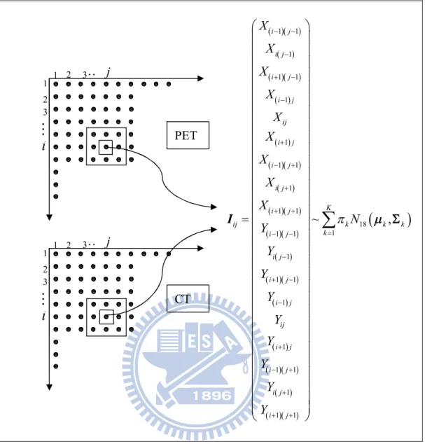
j PET CT

Next, the 1st and 2nd order spatial dependence are considered in GMM. The 1st order spatial dependence is to add the four adjacent points of each pixel on PET and CT images. A ten-dimensional GMM can be used to fit the data (PET and CT). The 2nd order spatial dependence is to add the eight points surrounding each pixel on PET and CT images. An eighteen-dimensional GMM can be used to fit the data (PET and CT). They are shown as follows:

Figure 2.3. 2: The 1st order spatial dependence in GMM.

i



3 3 j 2 1 2 1 j

i



3 3 j 2 1 2 1                





1 1 1 1 10 1 1 1 1 1 ~ , i j i j ij i j K i j ij k k k k i j i j ij i j i j X X X X X N Y Y Y Y Y                                               



I   j PET CT

Figure 2.3.3: The 2nd order spatial dependence in GMM.

2.3 Determine the Initial Parameters of GMM

The different initial values and number of clusters affect the clustering results in a GMM significantly. We will discuss how to select initial values of the GMM in this section.

Kernel density estimation (KDE) is a non-parametric approach to estimate the density function of data (Sheather and Jones, 1991). For a one-dimensional GMM, KDE can be applied to solve the issue of selecting initial values and the initial number of clusters. The K

i



3 3 j 2 1 2 1 j

i



3 3 j 2 1 2 1                                        





1 1 1 1 1 1 1 1 1 1 1 1 18 1 1 1 1 1 1 1 1 1 1 1 1 1 ~ , i j i j i j i j ij i j i j i j K i j ij k k k k i j i j i j i j ij i j i j i j i j X X X X X X X X X N Y Y Y Y Y Y Y Y Y                                                           _{ }                                



I   j PET CT

number of clusters K can be determined. The means and standard deviations of GMM can be determined by high peaks and low peaks. It is based on the 68-95-99.7 rule from a Gaussian distribution that about 99.7% data lie within the interval



3 , 3



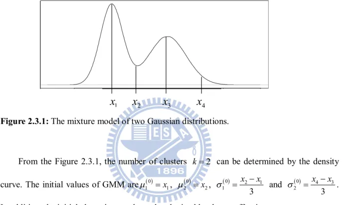
. The following is a basic example that shows a procedure to select the initial values of the GMM.

Figure 2.3.1: The mixture model of two Gaussian distributions.

From the Figure 2.3.1, the number of clusters k 2 can be determined by the density curve. The initial values of GMM are₁ 0 x₁,  ₂0 x₂,  0 2 1

1 3 x x    and  0 4 3 2 3 x x    .

In addition, the initial clustering result can be obtained by the cutoff point x . ₂

For a multi-dimensional GMM, we can reduce the data to one-dimension by averaging them. The initial clustering result can obtained by the cutoff points (low peaks) of the kernel density curve. And we use maximum likelihood estimator (MLE) of Multivariate Gaussian distribution to estimate the parameters of the multi-dimensional GMM. For k1, 2,,K,

  1 (0) I , xy k N I G xy k N    



( 0) , xy k xy I G k I N  



 3

x

1

x

x

₂

x

₄

(0) ( )( ) , xy k T xy k xy k I G k I I N    



  

where G represents the _k kth group, I_xy is d-dimensional vector.

In this study, Gaussian kernel functions are used to estimate the density function of image data. The bandwidth of KDE is determined by the program code of "density" in software R (Silverman,1986).

2.4 Bayesian Information Criterion for Model Selection

Bayesian information criterion (BIC) is a criterion for model selection developed by Schwarz (1978). It is similar to Akaike information criterion (AIC) (Akaike, 1974). The difference between BIC and AIC is that the penalty of the BIC for additional parameters is stronger than the penalty of the AIC. They are defined as follows:

 

2 log 2 AIC  L  p

 

 

2 log log BIC  L p N

where p is the number of free parameters, L is maximized value of likelihood function for the estimated model, and N is the number of data. The values of AIC and BIC are the same when the sample size N 7.389. When the sample size is greater than 7.389, the penalty term in BIC is greater than the AIC. Since the size of the image data are larger than 7.389, we will use BIC to select model. Given several estimated models, the model with the lower value of BIC is preferred. Hence, the number of clusters for GMM can be determined by the model with the minimum value of BIC.

intensity on images. CT, however, has a better outlining effect. The profiles of organs can be observed very clearly on CT images. We can combine the advantages of PET and CT. And we take weighed sum of PET and CT images to form one image as follow.









FusionPET 1 CT,  0, 1 .

In this study, let  0.5. That is, we take the average of PET and CT images to form fusion images. In addition, before we fused PET and CT images, we normalized the images between 0 and 1.

2.6 F-measure

In a statistical classification task, F-measure is a measure of testing accuracy (van Rijsbergen, 1979). It combines the precision (or we called Predicted Positive Value , PPV) and recall (or we called True Positive Rate, TPR) to form a single measure. Precision could be seen a measure of exactness and recall could be seen a measure of completeness. They are defined as following.

Table 2.6.1: The 2 2 contingency table of the real and estimated result. Real result

True False

True True Positive (TP) False Positive (FP) Estimated result

False False Negative (FN) True Negative(TN)

TP Precision , TP FP   TP Recall , TP FN  





2 Precision Recall . Precision Recall F    

The F-measure could be interpreted as the harmonic mean of precision and recall. It has the best performance when the value is 1 and worst performance when the value is 0.

2.7 Procedure

In this study, we have five procedures to segment the images shown as follows. And we will compare the accuracy of these methods by phantom study on Chapter 3.

Procedure 1: PET + GMM

Use one-dimensional GMM to segment PET images only. Procedure 2: Fusion + GMM

Use one-dimensional GMM to segment fusion images of PET and CT. Procedure 3: GMM (PET & CT)

Use two-dimensional GMM to segment PET/CT images. Procedure 4: 1st order spatial dependence in GMM (PET & CT)

Use the 1st order spatial dependence in GMM to segment PET/CT images. Procedure 5: 2nd order spatial dependence in GMM (PET & CT)

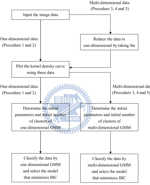
Figure 2.7.1: The procedure of segmenting images. One-dimensional data (Procedure 1 and 2) One-dimensional data (Procedure 1 and 2) (Procedure 3, 4 and 5) Plot the kernel density curve

using these data Input the image data

Reduce the data to one-dimensional by taking the

Determine the initial parameters and initial number

of clustersof one-dimensional GMM

Classify the data by one-dimensional GMM

and select the model that minimizes BIC

(Procedure 3, 4 and 5) Multi-dimensional data

Determine the initial parameters and initial number

of clustersof multi-dimensional GMM

Classify the data by multi-dimensional GMM

and select the model that minimizes BIC

Chapter 3 Phantom Study

The torso phantom data wereprovided by Dr. Tai-Been Chen from I-Shou University. It is designed for comparing the accuracy of different segmenting methods in this study. The information of phantom container is shown below. The region of the simulated heart container is injected a large amount of medicine. This makes the image appear in high intensity on PET images.

Figure 3.1: The information of phantom container.

PET and CT both have 114 slices where pixel size is 256 256 in the phantom experiment. The PET images which contain high intensity identify the area with high activity in the simulator. Different segmenting methods are used to segment the region of the highest activity in the simulator. The aim of this phantom study is to compare the accuracy of the highest region by these different segmenting methods. The following is the 43th slice of PET and CT images.

Figure 3.2: (A) The 43th slice of 114 PET images. (B) The 43th slice of 114 CT images.

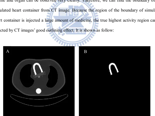
The region of high activity can be observed in the PET image. From CT image, the profile and organ can be observed very clearly. Therefore, we can find the boundary of the simulated heart container from CT image. Because the region of the boundary of simulated heart container is injected a large amount of medicine, the true highest activity region can be selected by CT images’ good outlining effect. It is shown as follow:

Figure 3.3: (A) The boundary of simulated heart container can be found from CT images. (B) The region of the true highest activity of 43th slice of CT image.

A B

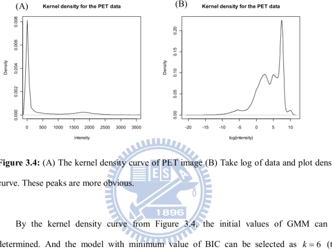
After obtaining the true highest activity region, we can compare the accuracy by F-measure (van Rijsbergen, 1979). First, the GMM is used to segment PET images. The following is kernel density curve of PET image data.

0 500 1000 1500 2000 2500 3000 3500 0 .0 0 0 0 .0 0 2 0 .0 0 4 0 .0 0 6 0 .0 0 8

Kernel density for the PET data

intensity D e n s it y -20 -15 -10 -5 0 5 10 0 .0 0 0 .0 5 0 .1 0 0 .1 5 0 .2 0

Kernel density for the PET data

log(intensity) D e n s it y

Figure 3.4: (A) The kernel density curve of PET image (B) Take log of data and plot density curve. These peaks are more obvious.

By the kernel density curve from Figure 3.4, the initial values of GMM can be determined. And the model with minimum value of BIC can be selected as k 6 (the number of clusters) from Figure 3.5 shown as follow.

7 3 8 0 0 0 7 4 0 0 0 0 7 4 2 0 0 0 7 4 4 0 0 0 7 4 6 0 0 0 7 4 8 0 0 0 PET B IC (A) (B)

The results of segmenting PET image by GMM shown as following. It obviously overestimates the real highest region.

Figure 3.6: k 6, The result of segmenting PET image by GMM with KDE.

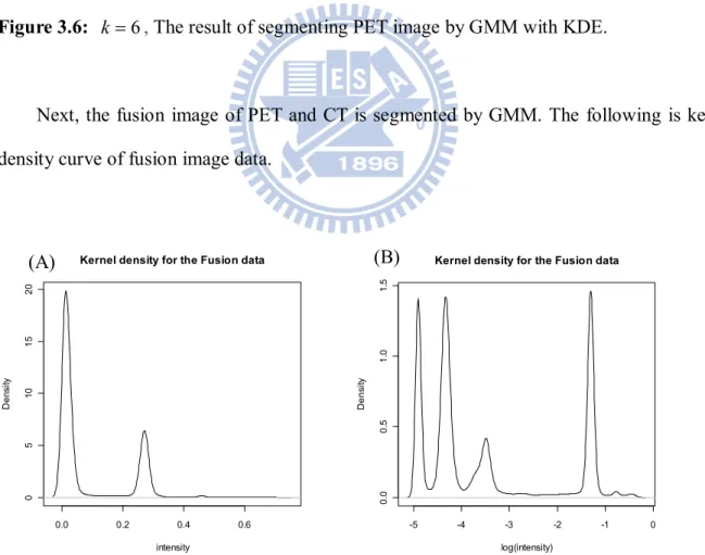
Next, the fusion image of PET and CT is segmented by GMM. The following is kernel density curve of fusion image data.

0.0 0.2 0.4 0.6 0 5 1 0 1 5 2 0

Kernel density for the Fusion data

intensity D e n s it y -5 -4 -3 -2 -1 0 0 .0 0 .5 1 .0 1 .5

Kernel density for the Fusion data

log(intensity) D e n s it y

Figure 3.7: (A) The kernel density curve of fusion image of PET and CT. (B) Take log of data and plot density curve. These peaks are more obvious.

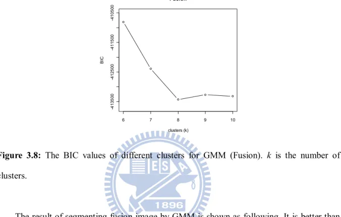
The initial values of GMM can be determined by the kernel density curve from Figure 3.7. And the model with minimum value of BIC can be selected as k 8 from Figure 3.8 shown as follow. 6 7 8 9 10 -4 1 3 5 0 0 -4 1 2 5 0 0 -4 1 1 5 0 0 -4 1 0 5 0 0 Fusion clusters (k) B IC

Figure 3.8: The BIC values of different clusters for GMM (Fusion). k is the number of clusters.

The result of segmenting fusion image by GMM is shown as following. It is better than the result of only implementing segmenting PET image at the highest region.

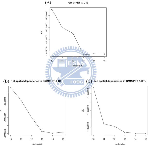
Finally, the two-dimensional GMM is fitted to the PET and CT data. And the 1st order and the 2nd order spatial dependence are used to in GMM as shown Figure 2.3.2 and Figure 2.3.3 on Chapter 2. The followings are the BIC values of different clusters of these three methods. 10 11 12 13 14 15 -1 0 2 5 0 0 0 -1 0 2 0 0 0 0 -1 0 1 5 0 0 0 -1 0 1 0 0 0 0 GMM(PET & CT) clusters (k) B IC 10 11 12 13 14 15 -6 0 8 0 0 0 0 -6 0 7 0 0 0 0 -6 0 6 0 0 0 0

1st spatial dependence in GMM(PET & CT)

clusters (k) B IC 10 11 12 13 14 15 -1 1 3 0 0 0 0 0 -1 1 2 6 0 0 0 0 -1 1 2 2 0 0 0 0

2nd spatial dependence in GMM(PET & CT)

clusters (k)

B

IC

Figure 3.10: The BIC values of different clusters. (A) GMM(PET & CT). (B) 1st spatial dependence in GMM(PET & CT). (C) 2nd spatial dependence in GMM(PET & CT).

(A)

From Figure 3.10, the cluster sizes can be selected k 13 for GMM(PET & CT), and k 14 for the 1st and 2nd spatial dependence GMM. These clustering results and accuracy are shown as following.

Figure 3.11: (A) k 13, the result of GMM (PET & CT). (B) k 14, the result of 1st spatial dependence GMM(PET & CT). (C) k 14, the result of 2nd spatial dependence GMM (PET & CT).

A

C B

Table 3.1: Comparison for the accuracy of the highest activity region of different methods by F-measure.

Recall (TRR) Precision (PPV) F-measure

PET + GMM 1.0000 0.5256 0.6891

Fusion + GMM 0.9682 0.9346 0.9511

GMM (PET&CT) 0.8962 0.9976 0.9442

1st order spatial GMM (PET&CT) 1.0000 0.7307 0.8444 2nt order spatial GMM (PET&CT) 0.9322 0.9692 0.9503

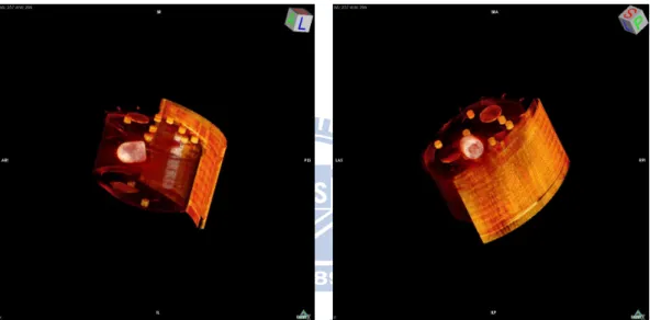
The comparison from Table 3.1 shows that the results of Fusion + GMM, GMM (PET&CT), 1st order spatial GMM (PET&CT) and 2nd order spatial GMM (PET&CT) all have higher accuracy than PET + GMM. Although GMM (PET&CT), the 1st and 2nd order spatial GMM (PET&CT) have slightly lower F-measure values than Fusion + GMM, they provided more information for the data. We can find the correlation of PET and CT on the regions of interesting. The correlation of the result of PET and CT could be used to detect the association pattern between the pixels of these two images. The correlation is positive as the area of a PET image has high (or low) isotope radioactivity and the area of a CT image has high (or low) X-ray absorption overlap very much. The correlation is negative as the area of a PET image with high (or low) isotope radioactivity and the area of a CT image with low (or high) X-ray absorption overlap very much. In addition, the correlations of neighbor points on PET and CT images also can be obtained by using spatial dependence in GMM. The following is some correlations of PET and CT on the result of using 2nd order spatial dependence in GMM.

Figure 3.12: The red regions show different correlations of PET and CT on the result of using 2nd order spatial dependence in GMM. (A) The correlation is -0.7575. (B) The correlation is 0.3704. (C) The correlation is -0.7540.

From Figure 3.12, the correlations of (A) and (C) are negative. It represents that the area of the PET image with high (or low) isotope radioactivity and the area of the CT image with low (or high) X-ray absorption overlap very much.

(C) A

Chapter 4 Conclusions

The information of CT images is used when segmenting PET images in this study. Besides segmenting fusion images of PET/CT and taking two-dimensional GMM fit the PET and CT data, we also used spatial dependence in GMM. These clustering results on the highest activity region all have better performance than the result of segmenting PET images only in Chapter 3. Besides the correlation of PET and CT, we also can find the correlations between neighbor points of PET and CT on the regions of interesting by using spatial dependence in GMM. Therefore, the model using spatial dependence is preferred in this phantom experiment since it provides more information for the data.

For further investigation, these methods can be tested for the stability of the performances with more phantom studies. Furthermore, it also could be applied in empirical study and judged by medical experts in the future.

Reference

[1] Akaike, H. (1974). A new look at the statistical model identification. IEEE Trans.

Automat. Ontr., 19, 716-723.

[2] Dempster, A.P., Laird, N.M., Rubin, D.B. (1977). Maximum likelihood from incomplete datavia the EM algorithm (with discussion). Journal of the Royal Statistical Society, B, 39, 1-38.

[3] Engel, J., Herrmann, E., Gasser, T. (1994). An iterative bandwidth selector for kernel estimation of densities and their derivatives. Journal of Nonparametric Statistics, 4, 21–34.

[4] Hsiao, I.T., Rangarajan, A., Gindi, G. (1998). Joint-Map Reconstruction/Segmentation for transmission Tomography Using Mixture-Model as Priors. Proc. IEEE Nuclear

Science Symposium and Medical Image Conference, 3, 1689-1693.

[5] Chiang H.Y. (2004). Segmentation of Dynamic MicroPET Images by K-mean and Mixture Methods. Master’s thesis, Institute of Statistics National Chiao Tung University.

[6] McLachlan, G.J., Basford, K.E. (1988). Mixture Model: Inference and Applications to

Clustering. Marcel Dekker, New York.

[7] Ye M.C. (2009). Segmentation of PET/CT images by Flexible Mixture Models and Comparison with K-means and Gaussian Mixture Models. Master’s thesis, Institute of Statistics National Chiao Tung University.

[8] Olinger, J.M., Fessler, J.A. (1997). Positron emission tomography. IEEE Signal

Processing Magazine, 14, 43-55.

kernel density estimation. Journal of Royal Statistics Society. B, 53, 683-690. [11] Silverman, B. W. (1986) Density Estimation. Chapman and Hall, London.

[12] Chen T.B. (2007). Statistical Applications of Maximized Likelihood Estimates with the Expectation-Maximization Algorithm for Reconstruction and Segmentation of MicroPET and Spotted Microarray Images. Ph.D. Dissertation, Institute of Statistics National Chiao Tung University.

[13] Townsend, D. W., Carney, J.P., Yap, J.T, Hall, N. C. (2004). PET/CT Today and Tomorrow. The Journal of Nuclear Medicine, 45, 4S-14S.

[14] Van Rijsbergen, C. J. (1979). Information Retrieval. London. 2nd Edition. Butterworth. London, England.

[15] Vardi, Y., Shepp, La., Kaufman, L. (1985). A statistical model for positron emission tomography. Journal of the American Statistics Association, 80, 8-20.

[16] Wong, K.P., Feng D., Meikle, S.R., Fulham, M.J. (2002). Segmentation of Dynamic PET Images Using Cluster Analysis. IEEE Transactions on Nuclear Science, 49, 200-207.