國立交通大學交通運輸研究所
碩士論文
不可儲存商品之生產績效衡量--整合式資料包絡分析模式
An Integrated Data Envelopment Analysis Model to
Evaluate the Performance of Non-storable Commodities
研 究 生:閻姿慧
9436505中 華 民 國 九十六 年 六 月
指導教授: 藍武王 博士
邱裕鈞 博士
不可儲存商品之生產績效衡量 -- 整合式資料包絡分析模式
研究生:閻姿慧 指導教授: 藍武王博士
邱裕鈞博士
國立大學交通運輸研究所
摘要
在評估不可儲存商品(如運輸服務)之生產績效時,由於生產效率與生產效 果之績效值並不等同,故應同時衡量兩部分,方不至於偏頗。當不可儲存商品一 旦生產且有一部分產出未能同時被消費時,則其生產效果(指技術效率與服務效 果的綜合效果)的績效值將小於生產效率的績效值。有鑑於此,本研究試圖建構 一整合式資料包絡分析 (Integrated Data Envelopment Analysis; IDEA) 模 式,以同時求解技術效率及服務效果的績效值。本 IDEA 模式可同時決定投入變 數、生產變數及消費變數的參數值,亦可證明具有「合理性」及「唯一性」。經 個案分析結果顯示,本 IDEA 模式的鑑別力較傳統 DEA 模式高。另,本文進一步 建構一般化 IDEA 模式,可看出權重變動對各個 DMU 之影響,俾提出更多改善效 率之方法。 關鍵字:整合式資料包絡分析模式,不可儲存商品,技術效率,技術效果。An Integrated Data Envelopment Analysis Model to
Evaluate the Performance of Non-storable Commodities
Student: Barbara T. H. Yen Advisors: Dr. Lawrence W. Lan
Dr. Yu-Chiun Chiou
Institute of Traffic and Transportation
National Chiao Tung University
Abstract
Efficiency and effectiveness for non-storable commodities such as transport services represent two distinct measurements. When such commodities are produced and a portion of which are not consumed instantaneously, the technical effectiveness (a combined effect of technical efficiency and service effectiveness) would be likely less than the technical efficiency. Based on this, this thesis attempts to develop an integrated data envelopment analysis (IDEA) model that can jointly determine the overall efficiency from the aspects of technical-efficiency, service-effectiveness, and technical-effectiveness. The core logic for the proposed IDEA model is to simultaneously determine the virtual multipliers associated with the variables of factor production and consumption. The underlying properties of reasonability and uniqueness of the proposed IDEA model are proven. The applicability of the proposed model is also demonstrated with a case study. It shows that our proposed IDEA model has higher discrimination power than the conventional separated DEA models.
Key Words: integrated DEA model, non-storable commodities, technical efficiency,
致謝
兩年的光陰悄悄飛逝,終於到了道離別的一刻,心中有滿足也有失落,滿足 於學業的完成,失落在分離即將到來。在交通大學的兩年中,結識了許多影響深 遠的好朋友以及尊長,在此謹以文字獻給陪伴我度過這兩年時光的大家。 首先,感謝指導教授 藍武王老師以及 邱裕鈞老師,在兩年之中給予我的諸 多指導與啟發。交通領域對我而言完全陌生,初入研究所的我是一張白紙,是由 藍老師在這張白紙上畫上第一道色彩,為我啟蒙,讓我見識到這個領域的精深廣 博。藍老師在這兩年當中给予我的不僅只有做學問的方法,還傳受了我許多禮儀 規範、做人處事的原則以及道理,最難能可貴的是老師總是以身作則。老師嚴以 律己的態度,讓我們有最好的典範可以參考、學習。做學問是一條無止盡的道路, 非常慶幸可以在這兩年中有藍老師的相伴與指導,相信這兩年會是我收穫最大的 兩年。若說藍老師領我入門,那那麼邱老師就是那枝負責點綴色彩的筆。邱老師 總是用最積極的態度與我們相處,教導我們如何做學問,讓我領略學問之深度之 廣泛,也常常給予我鼓勵與督促,總讓我們在做學問之餘,處處可以發現老師對 我們的關心與照顧。因此,在此深深感謝兩位老師。 在研究所兩年當中,非常感謝馮正民教授、徐淵靜教授、汪進財教授、黃台 生教授、黃承傳教授、許鉅秉教授以及陳穆臻教授對我們的教導與啟發。論文口 試與審查期間,承蒙胡均立教授以及游明敏撥冗細審,並且給予我許多寶貴之意 見,使本論文更加完善,在此非常感謝兩位老師。此外,特別感謝胡均立老師給 予我諸多額外的意見與指導,不論是在課堂中或是口試期間,本篇論文在其嚴格 的專業控管下甄於完美。 回想這兩年中,從大家一起進入研究所的那天,就開啟我們彼此的友誼之 窗,大家在這兩年中總是不吝惜對彼此伸出援手,互相幫忙互相扶持,謝謝大家 在這兩年中的陪伴,讓我知道同學之間的情誼可以這樣的深刻,如此的銘心,很 不想要互道珍重,但是大家有各自美好的前程,也做好展翅高飛的準備,所以我 預祝大家前程似錦、飛黃騰達。最後感謝你們陪我度過這兩年快樂又艱辛的日子。 心中尚有千言萬語未盡,想要感謝的人也太多,你們在我的生命中皆留下了 無可磨滅之痕跡,希望你們事事順心,身體健康。最後,感謝一路在我背後支持 我的家人,讓我得以順利完成學業,你們事我最大的動力來源,爸爸和媽媽無條 件的支持與付出讓我努力的很快樂,妹妹和弟弟的幫助讓我如虎添翼,所以在此 為你們的付出獻上十二萬分敬意。 2007 年 6 月 于台北 交通大學Table of Contents
1.
Introduction... 1
1.1.
Background ...1
1.2.
Purpose ...3
1.3.
Framework and organization...4
2.
Literature review ... 5
2.1.
Applications of DEA in transportation...5
2.1.1. Air transportation ... 5
2.1.2. Maritime transportation ... 6
2.1.3. Transit... 6
2.1.4. Railway ... 9
2.2.
DEA modeling ...10
2.3.
Comparisons of DEA with other methods...11
2.4.
Summary ...12
3.
Methodology ... 19
3.1.
Conventional DEA models ...19
3.1.1. CCR ... 19
3.1.2. BCC... 22
3.2.
Proposed IDEA models ...23
3.2.1. Proposed models ... 23
3.2.1.1. Cost efficiency...23
3.2.1.2. Service effectiveness...24
3.2.1.3. Integrated model ...25
4.
Properties of the proposed IDEA Models... 29
4.1.
Rationality ...29
4.1.1. Rationality for ICCR model ... 29
4.1.2. Rationality for IBCC model ... 30
4.2.
Uniqueness...32
5.
Case study ... 34
5.1.
Data ...34
5.2.
Efficiency scores...35
5.4.
Weight analysis for generalized IDEA model ...38
5.5.
Overall weight analysis ...55
6.
Conclusions and suggestions... 59
6.1.
Conclusions...59
6.2.
Suggestions ...60
List of Tables
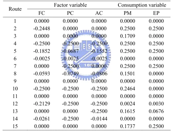
Table 1 Summary of literature review... 14 Table 2 Basic characteristics of the 15 domestic routes operated by Airline U 34 Table 3 Data of 15 domestic routes operated by Airline U (in %)... 35 Table 4 Scores of overall and separate efficiencies of each route under CRS.. 36 Table 5 Scores of overall and separate efficiencies of each route under VRS . 37 Table 6 Returns to scale of each route ... 37 Table 7 Slack values of factor and consumption variables under CRS ... 38 Table 8 The technical efficiency and service effectiveness of DMU 1 with
various weight combinations ... 40 Table 9 The technical efficiency and service effectiveness of DMU 2 with
various weight combinations ... 41 Table 10 The technical efficiency and service effectiveness of DMU 3 with
various weight combinations ... 42 Table 11 The technical efficiency and service effectiveness of DMU 4 with
various weight combinations ... 43 Table 12 The technical efficiency and service effectiveness of DMU 5 with
various weight combinations ... 44 Table 13 The technical efficiency and service effectiveness of DMU 6 with
various weight combinations ... 45 Table 14 The technical efficiency and service effectiveness of DMU 7 with
various weight combinations ... 46 Table 15 The technical efficiency and service effectiveness of DMU 8 with
various weight combinations ... 48 Table 16 The technical efficiency and service effectiveness of DMU 10 with
various weight combinations ... 49 Table 17 The technical efficiency and service effectiveness of DMU 9 with
various weight combinations ... 50 Table 18 The technical efficiency and service effectiveness of DMU 11 with
various weight combinations ... 51 Table 19 The technical efficiency and service effectiveness of DMU 12 with
various weight combinations ... 52 Table 20 The technical efficiency and service effectiveness of DMU 13 with
various weight combinations ... 53 Table 21 The technical efficiency and service effectiveness of DMU 14 with
various weight combinations ... 54 Table 22 The technical efficiency and service effectiveness of DMU 15 with
various weight combinations ... 55 Table 23 Technical efficiency of each DMU with various weight combinations ... 56 Table 24 Service effectiveness of each DMU with various weight combinations ... 57
List of Figures
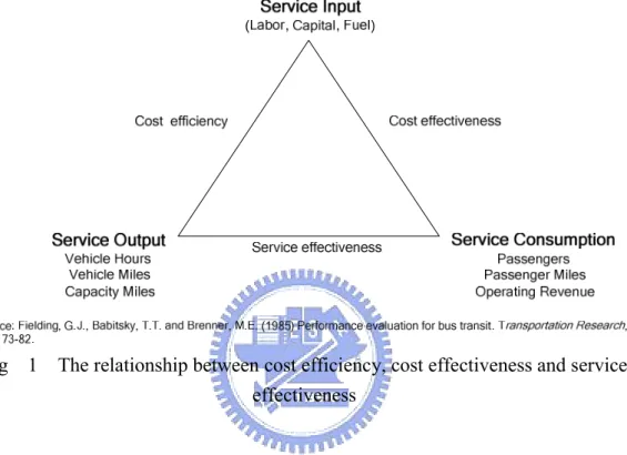
Fig 1 The relationship between cost efficiency, cost effectiveness and service effectiveness ...2
Fig 2 Research flowchart...4
Fig 3 The analysis framework...5
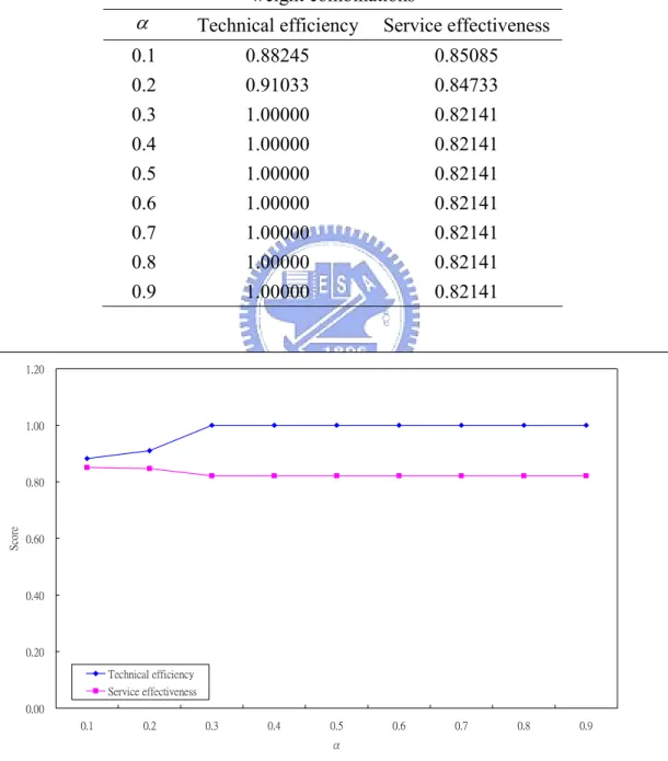
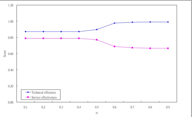
Fig 4 The shapes of technical efficiency and service effectiveness of DMU 1 with various weight combinations...40
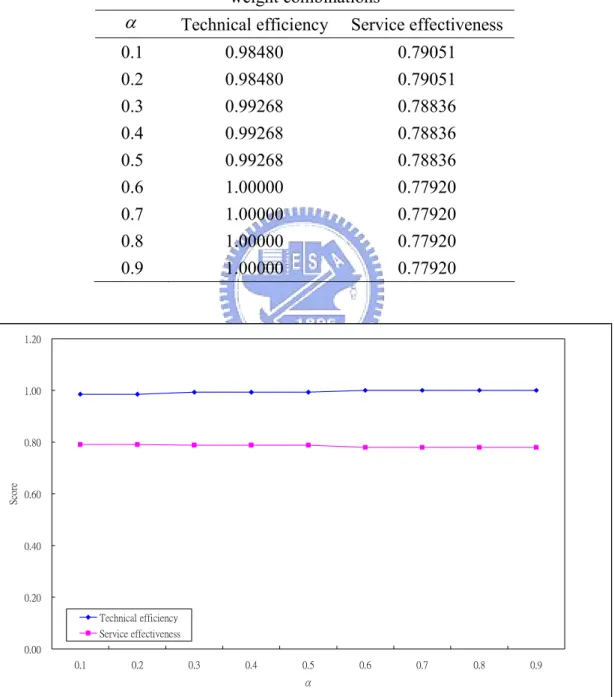
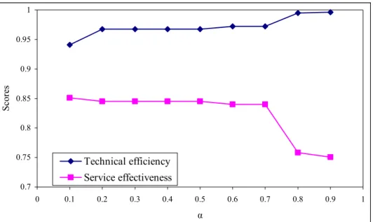
Fig 5 The shapes of technical efficiency and service effectiveness of DMU 2 with various weight combinations...41
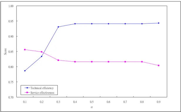
Fig 6 The shapes of technical efficiency and service effectiveness of DMU 3 with various weight combinations...43
Fig 7 The shapes of technical efficiency and service effectiveness of DMU 4 with various weight combinations...44
Fig 8 The shapes of technical efficiency and service effectiveness of DMU 5 with various weight combinations...45
Fig 9 The shapes of technical efficiency and service effectiveness of DMU 6 with various weight combinations...46
Fig 10 The shapes of technical efficiency and service effectiveness of DMU 7 with various weight combinations...47
Fig 11 The shapes of technical efficiency and service effectiveness of DMU 8 with various weight combinations...48
Fig 12 The shapes of technical efficiency and service effectiveness of DMU 10 with various weight combinations...49
Fig 13 The shapes of technical efficiency and service effectiveness of DMU 9 with various weight combinations...50
Fig 14 The shapes of technical efficiency and service effectiveness of DMU 11 with various weight combinations...51
Fig 15 The shapes of technical efficiency and service effectiveness of DMU 12 with various weight combinations...52
Fig 16 The shapes of technical efficiency and service effectiveness of DMU 13 with various weight combinations...53
Fig 17 The shapes of technical efficiency and service effectiveness of DMU 14 with various weight combinations...54
Fig 18 The shapes of technical efficiency and service effectiveness of DMU 15 with various weight combinations...55
Fig 19 The shapes of technical efficiency of Each DMU with various weight combinations ...56
Fig 20 The shapes of Service effectiveness of Each DMU with various weight combinations ...57
1. Introduction
1.1. Background
Data Envelopment Analysis (DEA) is a technique that provides a comprehensive insight into how comparatively well an organization performs. It can be used to rank quality level and analyze the performance with multiple inputs and outputs simultaneously. DEA imposes neither a specific functional relationship between production output and input, nor any assumptions on the specific statistical distribution of the error terms. DEA can be defined as a nonparametric method of measuring the efficiency of a Decision Making Unit (DMU).
DEA can be directly applied to evaluate the relative performance of the companies producing storable products, since these products can be stored for re-sell in the future even they cannot be sold instantly. The operating performance of such organization can be represented by its technical efficiency which is equivalent to technical effectiveness. However, in evaluating the industry producing non-storable products, such as transportation industry, technical efficiency only represent one aspect of the performance. The manager of a transport company might even more concern about technical effectiveness, which measures how many revenue passenger-miles or ton-miles are generated. Accordingly, Fielding (1985) proposed an analytical framework to evaluate the performance of a transportation industry by three aspects: cost-efficiency, service-effectiveness and cost-effectiveness, as depicted in Fig.1. In order to completely and fairly evaluate the relative performance of a transport organization, many studies employed DEA to evaluate the efficiency and effectiveness under respective aspect independently. For instance, Chiou and Chen (2006) employed DEA to evaluate the relative performance of domestic air routes operated by one airline under these three aspects respectively. However, some contradictory improvement suggestions were proposed based on the evaluating results of three independent DEA model. Lan and Lin (2003) employed a two-stage DEA model to evaluate the relative efficiency of various rail companies. They first use input-oriented DEA model to evaluate the cost-efficiency of these companies, then employ output-oriented DEA model to evaluate the service-effectiveness of these companies. The efficiency scores of cost-effectiveness aspect can be obtained as the product of the scores of cost-efficiency and service-effectiveness. Although this approach (two-stage DEA model) will not generate conflicting improvement suggestions, an unrealistic assumption have been made that the organization can be clearly divided into two departments: production and sales and be evaluated separately without any integration or coordination.
These unrealistic evaluation results of abovementioned studies are mainly rooted from their separate evaluation procedure. Therefore, a one-stage evaluation procedure is extremely essential to evaluate the performance of transportation industry for avoiding these problems. This study aims to develop an integrated DEA model to simultaneously evaluate the performance of transportation industry under three various aspects within one stage.
Fig 1 The relationship between cost efficiency, cost effectiveness and service effectiveness
1.2. Purpose
Based on the abovementioned background and motivation, the main purposes of this study are listed as follows:
1. Review and summarize the related studies in evaluating the performance of transportation industry by applying DEA model.
2. Develop and validate a one-stage DEA model for simultaneously evaluating the relative performances of transportation organizations under three aspects of cost-efficiency, service-effectiveness and cost-effectiveness.
3. Propose an effective and efficient solution algorithm for the one-stage DEA model.
4. Apply the proposed one-stage DEA model to evaluate the relative performances of domestic air routes and compare the results with those of Chiou and Chen(2006).
1.3. Framework and organization
The flowchart of this study is shown in Figure 2. Following this chapter, the thesis is organized as follows. Chapter 2 reviews some relevant literature on DEA. Chapter 3 introduces our proposed integrated DEA models. The essential
properties of the proposed models are proven in Chapter 4. A case study with the proposed IDEA models is conducted in Chapter 5. Final conclusions and future study are addressed in Chapter 6.
2. Literature review
2.1. Applications of DEA in transportation
DEA model has been widely applied to evaluate the relative performance of transportation industries, such as air transportation, maritime transportation, transit, railway, etc. The related studies are reviewed and summarized as follows.
2.1.1. Air transportation
Adler and Berechman (2001) use DEA to determine the relative efficiency or quality ranking of various West-European and other airports. The main source of data for this study was a questionnaire whose objective was to evaluate the quality level of 26 airports.
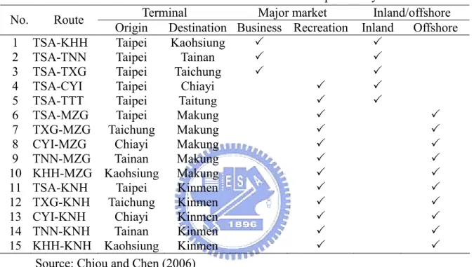
Chiou and Chen (2006) employ DEA approach to evaluate the performance of domestic air routes from the perspectives of cost efficiency, cost effectiveness and service effectiveness. The cost efficiency indicates the relative efficiency in the production; while the service effectiveness stands for the relative efficiency in the sale. The cost effectiveness therefore represents a combined effect of the relative efficiency in both production and sale. This paper adopts this framework to evaluate air route performance.
There are three input variables: fuel cost (FC), personnel cost (PC), including the salaries of cabin and ground-handling crews, and aircraft cost (AC), including maintenance costs, depreciation costs and interest payments. The production variables include number of flights (FL) and seat-mile (SM). The service variables include passenger-mile (PM) and embarkation passengers (EP), as shown in Fig. 3. This study also uses Tobit regression to identify variables are significant or not.
Peck et al. (1998) focus on discretionary maintenance strategies and their relationship to aircraft reliability, as measured by the percentage of scheduled flights delayed because of mechanical problems. The methodology of data envelopment analysis employed to identify the various strategies employed by the major airlines over the time period 1990-1994. The output variable was defined to be the percentage of all scheduled flights arrivals delayed for mechanical reasons not including weather or scheduling problems. The input variables represent all of the reported non-overlapping categories of maintenance expenses.
Tzeng and Chiang (2000) propose a new efficiency measure in data envelopment analysis: the efficiency achievement measure. Comparing with the traditional radial measure and distance measure proposed by Chang and Guh (1995) using different sets of multipliers to compute the efficiency ratio, the efficiency achievement measure does so by using the common multipliers that obtained easily by solving fuzzy multiple objectives programming.
2.1.2. Maritime transportation
Tongzon (2001) applies DEA to provide an efficiency measurement for four Australian and twelve other international container ports. This study uses two output and six input measures of port performance. The output measures are cargo throughput and ship working rate. Based on the production framework, port inputs can be generalized as land, labor and capital. The major capital inputs in port operations are the number of berths, cranes and tugs. This study has shown the suitability of DEA for port efficiency evaluation.
2.1.3. Transit
Karlaftis (2003) uncovers production characteristics of transit firms by relating efficiency with production in a less constraining environment. In this study uses data envelopment analysis to rank efficient subsets of transit systems and then based on the results of the DEA analysis, build globally efficient frontier production functions. The results indicate that when jointly considered, there is an improvement on both the theoretical and empirical aspects of examining efficiency and production in transit systems.
Fielding et al. (1984) use three categories of statistics-service inputs, service outputs and service consumption-provided the framework to organize
the much larger set of data. Cost-efficiency indicators measure service inputs (labor, capital, fuel) to the amount of service produced (service outputs: vehicle hours, vehicle miles, capacity miles, service reliability). Cost-effectiveness indicators measure the level of service consumption (passengers, passenger miles, operating revenue) against service inputs. Finally, service-effectiveness indicators measure the extent to which service outputs are consumed. Fig. 1 portrays the organizing framework.
Odeck and Alkadi (2001) focus on the performance of Norwegian bus companies subsidized by the government. The performance is evaluated from a productive efficiency point of view. The framework is DEA approach to efficiency measurement. In this study, the output variables are seat kilometers, vehicle kilometers, passenger kilometers, and passengers and the input variables are the total number of seats (TS) offered by the company, fuel consumption in liters (FC) and equipment (EQ) such as oil and tires. The average bus company is found to be exhibiting increasing return to scale. This means that the average company is smaller than the optimal size.
Viton (1998) examines the claim that US bus transit productivity has declined in recent years. These systems operated either conventional motor-bus (MB) or demand-responsive (DR) services (or both), but no other form of public transit. This paper uses a piecewise-linear best-practice DEA production frontier, computed for multi-modal bus transit between 1988 and 1992. The outputs are vehicle-miles, vehicle hours and passenger trips.
The inputs come from three sources. First is a set of variables describing the situation in which the system finds itself. These include the average fleet age and the number of directional miles provided by the MB. Second, we use a number of conventional inputs: the fleet sizes, and the number of gallons of fuel. It distinguishes four kinds of labor inputs: the number of person-hours of transportation, maintenance, administrative, capital and labor used by each mode in providing service. The final inputs are those for which there is no obvious summary physical measure. For these we use a cost measure. In this category we have the cost of tires and other materials and supplies, of services, of utilities, and of insurance.
The results do not support the pessimistic view of changes in the industry because both the efficiency and productivity approaches suggest an
improvement.
Cowie and Asenova (1999) claim that the ideal output measure is passenger kilometers, unfortunately due to commercial sensitivity such figures are unavailable. Nevertheless, clearly related to passenger kilometers is operating revenue. The inputs for each company reflect capital and labor elements. Labor is simply the total staff employed, both management and operational. This study shows strong evidence of increasing returns for smaller companies. This study uses technical, managerial and organizational efficiency. The technical efficiency of each company is assessed by a comparison of all companies in the data set. The level of managerial efficiency however, can be further isolated from overall technical efficiency by separating DMUs into the different sets of interest. The difference between technical and managerial efficiency represents the level of inefficiency attributed to the organizational structure.
Karlaftis (2004) uses data envelopment analysis and globally efficient frontier production functions to investigate two important issues in transit operations: first, the relationship between the two basic dimensions of performance, namely efficiency and effectiveness; second, the relationship between performance and scale economies.
This study found that systems performing well in one dimension (e.g. efficiency) generally perform well in the other dimensions (e.g. effectiveness). This is important since the performance scores can be useful in describing transit system performance both for internal and external purposes.
This study uses two outputs: vehicle-miles (often referred to as ‘‘produced output type’’) and passenger-miles (often referred to as ‘‘consumed output type’’). Transit systems most frequently use three input quantities, namely labor, fuel, and capital to produce output.
As many authors have suggested (for example Fielding, 1987), vehicle-miles are related to service efficiency while ridership (and passenger-miles) are related to effectiveness; a combined vehicle-miles and ridership output is related to a ‘‘combined’’ or ‘‘overall’’ performance measure. As such, in this paper we estimate three separate sets of models, each of them utilizing the same inputs but different outputs: the first is an efficiency
model, using total annual vehicle-miles as output; the second is an effectiveness model, using total annual ridership as the measure of output; the third is a multi-output model using both annual vehicle-miles and annual ridership as outputs to capture the combined performance.
2.1.4. Railway
Lan and Lin (2003) adopt various DEA approaches to investigate the technical efficiency and service effectiveness for some selected 76 railways. This paper attempts to estimate both of the technical efficiency and service effectiveness for worldwide rail systems by employing two-stage DEA. At the technical efficiency analysis stage, we use input orientation DEA by selecting length of lines, number of locomotives and cars, and number of employees as inputs and train-kilometer as output. At the service effectiveness analysis stage, we use output orientation DEA by selecting train-kilometer as input and passenger-kilometer and ton-kilometer as outputs. In addition, we perform a technical effectiveness analysis with one-stage DEA by choosing the same input factors and outputs.
Conventional DEA approaches neither consider the environmental differences across the DMUs nor account for the statistical error (data noise) and slack effects. Thus, the comparison can be seriously biased because all DMUs are not brought into a common platform. Fried et al. (2002) proposed a three-stage DEA approach with consideration of the environmental effects and statistical noise, but they still did not adjust the slack effects. Lan and Lin (2005) propose a four-stage DEA approach with further adjustment of slack effects. The empirical results show that proposed four-stage DEA approach has slightly more reasonable efficiency and effectiveness scores than those measured by Fried’s three-stage DEA approach.
This paper measures the technical efficiency by selecting number of passenger cars per kilometer of lines, number of freight cars per kilometer of lines, and number of employees per kilometer of lines as input factors and passenger train-kilometer per kilometer of lines and freight-train-kilometer per kilometer of lines as output variables. In measuring the service effectiveness, on the other hand, we choose passenger-kilometers and ton-kilometers as two consumptions and passenger train kilometers and freight train-kilometers as two outputs.
2.2. DEA modeling
Yun et al. (2004) suggest a model called generalized DEA (GDEA) model, which can treat the basic DEA models (CCR model, BCC model and FDH model) in a unified way. GDEA model can make a quantitative analysis for inefficiency on the basis of surplus of inputs and slack of outputs.
DEA was suggested by Charnes, Cooper and Rhodes (CCR) which is concerned with the estimation of technical efficiency and efficient frontiers. The CCR model generalized the single output/single input ratio efficiency measure for each decision making unit to multiple outputs/multiple inputs situations by forming the ratio of a weighted sum of outputs to a weighted sum of inputs. Tulkens introduced a relative efficiency to non-convex free disposable hull (FDH) of the observed data, and formulated a mixed integer programming to calculate the relative efficiency for each DMU.
Gautam and Paul (2006) provide an alternative framework for solving DEA models which, in comparison with the standard linear programming (LP) based approach that solves one LP for each DMU. The method of projection, which we use, is Fourier–Motzkin (F–M) elimination. It is shown that the output from the F–M method improves on existing methods of (i) establishing the returns to scale status of each DMU, (ii) calculating cross-efficiencies and (iii) dealing with weight flexibility.
El-Mahgary and Lahdlma (1995) examine various two-dimensional charts for illustrating the DEA efficiency results. The identification of reference units provides a general framework that can be used to define guideline for the inefficient units. Visualizing such results should help decision-maker to better understand the result of a DEA assessment.
Cooper et al. (2001) examine two approaches that are presently available in the DEA literature for use in identifying and analyzing congestion. These two approaches are due to Färe et al. (Färe, R., Grosskopf, S., Lovell, C.A.K., 1985, The measurement of efficiency of production, Kluwer-Nijhoff Publishing, Boston, MA) and Cooper et al. (Cooper, W.W., Thompson, R.G., Thrall, R.M., 1996, Introduction: extensions and new developments in DEA, Annals of Operations research 66, 3-45). This study shows that FGL model might fail to give correct result.
Cherchye et al. (2001) respond the problem that FGL model fails to identify congestion in Cooper et al. examples. Because FGL model was originally proposed for measuring structural efficiency rather than detecting congestion.
2.3. Comparisons of DEA with other methods
Cullinane et al. (2006) apply the two leading approaches to efficiency measurement, DEA and SFA, to the same data set for the container port industry. This study suggests that a dynamic application of these frontier techniques, utilizing panel data approaches, may be more germane to ascertaining the relative efficiency levels of the international ports industry. In a dynamic context, technical efficiency can be separated not only from scale efficiency, but also from technological take-up. This paper rank order of the technical efficiency derived from applying the alternative DEA and SFA approaches ranges from 0.63 to 1.00, indicating that these approaches yield similar efficiency rankings. The hypothesis of constant returns to scale in the production frontier for the industry could not be rejected when applying the stochastic frontier model. The application of the same sort of hypothesis test to the results yielded by the application of the DEA model is not appropriate, however, as the mathematical programming nature of DEA means that the underlying model does not possess any statistical assumptions or properties per se. Applying the DEA approach does, however, yield the results that the terminals in the sample were found to exhibit a mix of decreasing, increasing and constant returns to scale at current levels of output. Compared with the stochastic parametric frontier approach, DEA imposes neither a specific functional relationship between production output and input, nor any assumptions on the specific statistical distribution of the error terms. In so doing, the data are believed to be able to “speak for themselves” and the DEA approach has the advantage of minimal specification error. However, the DEA model does not allow for measurement error or random shocks. Instead, all these factors are attributed to efficiency, a characteristic that inevitably leads to potential estimation errors. In this paper, the main objective of a port is assumed to be the minimization of the use of input(s) and maximization of the output(s). The inputs of this paper are terminal length (m), terminal area (ha), quayside gantry (number), yard gantry (number) and straddle carrier (number) and the output of this paper is container throughput (TEU).
frontier analysis to determine efficiency rations for European airports. The SFA might be more flexible then DEA as SFA includes a noise term. However, this study suggests that more attention has to be paid to the “explaining” inefficiency, either using a stochastic frontier model or DEA output because the inputs used are not “standard” variable inputs. That means in the short run, they cannot be fully flexible. The estimation result of SFA is similar to DEA result. It appears that most airports are operating under increase returns to scale.
Coelli and Perelman (1999) discuss and compare a number of the different methods that have been used to estimate multi-output distance functions. This study focus upon the three most commonly used estimation methods:
(1) A parametric frontier using linear programming methods;
(2) A non-parametric piece-wise linear frontier using the linear programming method known as data envelopment analysis (DEA); and (3) A parametric frontier using corrected ordinary least squares (COLS).
The three different estimation methods provide similar information on the relative productive performance. The correlations between the various sets of technical efficiency predictions are all positive and significant. Furthermore, the parameter estimates obtained using the two parametric estimates are also quite similar in many respects. Given these observations, it appears that a researcher can safely select one of these methods without too much concern for their choice having a large influence upon results.
2.4. Summary
Table 1 summarizes of the literature review, from which, one can notice several points. First, some papers only use technical efficiency to evaluate the performance of transportation. That means these papers do not consider non-storable characteristic of transportation industries. Second, some papers use two stages (technical efficiency and service effectiveness) to evaluate the performance for transportation industries, however, these papers calculate the efficiency and effectiveness scores independently. One shall calculate the efficiency scores and effectiveness at the same time because one is evaluating two different departments in one company. One should treat these two departments dependently. Third, from these papers, one could discover that most
of them use labor, capital and fuel as input variable and use vehicle miles and passenger miles as output and service variables.
In this study, we will use cost efficiency, service effectiveness and cost effectiveness to evaluate the performance for transportation industry. In order to treat these three parts as an interactively dependent group, we try to formulate an integrated model to measure these three performance scores at the same time.
Table 1 Summary of literature review
No Author Year Industry Approach Evaluating aspect Input variables Output variables Service variables Model DMU
terminal length terminal area quayside gantry yard gantry 1 Cullinane et al. 2006 Port DEA SFA Technical efficiency straddle carrier container throughput - CCR BCC Country
Terminal size Air transport movement aircraft parking positions
at the terminal Passenger movement remote aircraft parking
positions
number of check-in desks 2 Pels et al. 2001 Airport DEA
SFA
Technical efficiency
number of baggage claim
-
- BCC City
Operating cost Vehicle-miles travelled Number of vehicles Passengers
Gallons of fuel 3 Karlaftis 2003 Transit DEA Technical
efficiency
Total employees -
- CCR US City
Questionnaire Service satisfacting Haul charge
Connection times 4 Adler and
Berechman 2001 Airport DEA
Technical efficiency
Average delay time
Number of terminals Number of runways Distance to the nearest
major city-center number of berths, cranes
and tugs cargo throughput number of port authority
employees ship working rate 5 Tongzon 2001 Port DEA Technical
efficiency
terminal area of the ports -
- CCR City
Cost efficiency fuel cost number of flights passenger-mile personnel cost seat-mile embarkation passengers Service
effectiveness aircraft cost 6 Chiou and
Chen 2006 Airport DEA
Cost effectiveness - - -
CCR
BCC Airline labor vehicle hours passengers
Technical
efficiency capital vehicle miles passenger miles
fuel capacity miles operating revenue Service
effectiveness service reliability 7 Fielding et
al. 1984 Transit DEA
Technical effectiveness
-
- -
CCR US City
Non-interes expense Deposits Interest income plus
8 Yun et al 2004 Bank DEA GDEA Technical efficiency non-interest income - - CCR BCC FDH Bank
- labor expenses on
airframes flights arrivals delayed labor expenses on aircraft
engines for mechanical reasons expenditures on airframe repairs expenditures on engine repairs material expenditures on airframes
9 Peck et al. 1998 Airport DEA Technical efficiency
material expenditures on engines
-
- BCC Airlines
total number of seats seat kilometers fuel consumption vehicle kilometers consumption equipment passenger kilometers 10 Odeck and
Alkadi 2001 Transit DEA
Technical efficiency
- passengers
- BCC Bus company fleet sizes vehicle-miles
number of gallons of fuel passenger trips number of person-hours
of transportation vehicle hours 11 Philip A.
Viton 1998 Transit DEA
Technical efficiency
number of person-hours -
- BCC Transit industry
of maintenance number of person-hours
of administrative capital
the cost of tires and other materials
the cost of services the cost of utilities the cost of insurance
total staff employed operating revenue Technical
efficiency fleet size Managerial
efficiency 12 Cowie and
Asenova 1999 Transit DEA
Organisational efficiency
- -
- BCC Bus company
length of lines train-kilometer passenger-kilometer Technical
efficiency number of locomotives
and cars ton-kilometer number of employees
13 Lan and Lin 2003 Railway DEA
Service effectiveness - - - CCR BCC EXO CAT Railway
Lines passenger train-kilometer passenger-kilometers 14 Lan and Lin 2005 Railway DEA Technical
efficiency Passenger cars freight-train-kilometer ton-kilometers
BCC
Freight cars Stage) Service
effectiveness Employees - - total capital net operation revenue
number of employees passenger-kilometers 15 Tzeng and
Chiang 2000 Airport DEA
Technical efficiency
total number of seats
- CCR BCC
Airline company Number of vehicles vehicle-miles passenger-miles
Technical
efficiency gallons of fuel Total employees Service
effectiveness 16 Karlaftis 2004 Transit DEA
Technical effectiveness
-
- - BCC City
annual mean of monthly
data on staff€ levels passenger services available freight wagons freight services coach transport capacities
in tones
coach transport capacities in seats 17 Coelli and Perelman 1999 Railway DEA SFA COLS Technical efficiency
total length of lines
-
- BCC Company
EXO DEA: exogenously fixed inputs model
CAT DEA: To compare the performance measurements in a homogeneous environment can be formulated according to appropriate categorical variables. COLS: A parametric frontier using corrected ordinary least squares
3. Methodology
3.1. Conventional DEA models
DEA was initially developed as a method for assessing the comparative efficiencies of organizational units. The key feature which makes the units comparable is that they perform the same function in terms of the kinds of inputs they use and the types of outputs they produce.
DEA was first developed by Charnes et al. (1978), who generalized the single-output/single-input ratio efficiency measure for each DMU. The CCR model generalized the single output/single input ratio efficiency measure for DMU to multiple outputs/multiple inputs situations by forming the ratio of a weighted sum of outputs to a weighted sum of inputs. Based on the CCR model, Banker et al. (1984) suggested a model for estimating technical efficiency and scale inefficiency in DEA by adding convexity constrain. The BCC model relaxed the constant returns to scale assumption of the CCR model and made it possible to investigate whether the performance of each DMU was conducted in region of increasing, constant or decreasing returns to scale in multiple outputs and multiple inputs situations.
The main characteristics of DEA are that (i) it can be applied to analyze multiple outputs and multiple inputs without pre-assigned weights, (ii) it can be used for measuring a relative efficiency based on the observed data without knowing information on the production function.
Two basic DEA models are CCR model and BCC model. These two basic forms are illustrated as following.
3.1.1. CCR
DMU k is assumed to be evaluated. And there are i DMUs, each utilizes j kinds of inputs, (x1i,x2i,K,xji), and purchases r kinds of
outputs, )(y1i,y2i,K,yri . The efficiency of DMU k can be estimated by
v u Max ,
∑
∑
= = = m j kj j s r kr r k x v y u h 1 1 s.t. 1 1 1 ≤∑
∑
= = m j ij j s r ir r x v y u , i=1 L,2, ,n (1-1) 0 ≥ j v , j=1 L,2, ,m 0 ≥ r u , r =1 L,2, ,sThe model (1-1) is an input oriented programming problem, which can be formulated as output oriented problem by following programming.
μ ω, Min
∑
∑
= = = s r kr r m j kj j k y x g 1 1 μ ω s.t. 1 1 1 ≥∑
∑
= = s r ir r m j ij j y x μ ω , i=1 L,2, ,n (1-2) 0 ≥ j ω , j=1 L,2, ,m 0 ≥ r μ , r=1 L,2, ,sThen, one can transform above model (1-1) into an ordinary linear problem, show as following.
v u Max , =
∑
= s r kr r k u y h 1 s.t. 0 1 1 ≤ −∑
∑
= = m j ij j s r ir ry v x u , i=1 L,2, ,n (1-3) 1 1 =∑
= m j kj jx v , 0 ≥ j v , j=1 L,2, ,m0 ≥ r
u , r =1 L,2, ,s
Because model (1-3) is a linear problem, one can transform it into dual problem as follows. i z Min λ , z s.t. 0 1 ≥ −
∑
= n i i ij kj x zx λ , j=1 L,2, ,m (1-4) 0 1 ≥ + −∑
= n i i ir kr y y λ , r=1 L,2, ,s 0 ≥ i λ , i=1 L,2, ,nz is a scalar, which is the efficiency of kth firm, and it ranges from zero to unity. If z equals to one, the firm is efficient. And if z is less then one, the firm is inefficient.
One also can transform output oriented model (1-2) into linear problem (1-5) and then one can find its dual problem (1-6), show as follows.
μ ω, Min
∑
= = m j kj j k x g 1 ω s.t. 0 1 1 ≥ + −∑
∑
= = m j ij j s r ir ry ω x μ , i=1 L,2, ,n (1-5) 1 1 =∑
= s r kr ry μ , 0 ≥ j v , j=1 L,2, ,m 0 ≥ r u , r =1 L,2, ,s Dual problem, i z Max λ , φ s.t. 0 1 ≥ + ⋅ −∑
= n i i ir kr y y λ φ , r=1 L,2, ,s 0 1 ≥ −∑
= n i i ij kj x x λ , j=1 L,2, ,m (1-6)0 ≥ i
λ , i=1 L,2, ,n
3.1.2. BCC
Model (1-4) and model (1-6) are input and output oriented DEA models under the assumption of constant returns to scale (CRS) production technology. Then Banker, Charnes and Cooper (1984) relaxed this CRS constrain to variable returns to scale (VRS) technology by adding convexity constraint, as following models. Then one can get BCC input (1-7) and output oriented model (1-8) as following.
i z Min λ , z s.t. 0 1 ≥ −
∑
= n i i ij kj x zx λ , j=1 L,2, ,m (1-7) 0 1 ≥ + −∑
= n i i ir kr y y λ , r=1 L,2, ,s 0 ≥ i λ , i=1 L,2, ,n 1 1 =∑
= n i i λ i z Max λ , φ s.t. 0 1 ≥ + ⋅ −∑
= n i i ir kr y y λ φ , r=1 L,2, ,s 0 1 ≥ −∑
= n i i ij kj x x λ , j=1 L,2, ,m (1-8) 0 ≥ i λ , i=1 L,2, ,n 1 1 =∑
= n i i λOnce one knows the basic models for DEA, one can use these models to evaluate relative efficiency for each DMU. One usually uses two stages DEA to evaluate non-storable commodities. That means one uses input oriented DEA model to evaluate technical efficiency and use output oriented DEA model to evaluate service effectiveness.
From these two stages DEA, one would know how to improve the efficiency in each department. If one uses two stages DEA to calculate
the value of technical efficiency and service effectiveness respectively, it means one treats these two departments as independent. However, these two departments are dependent; namely, one cannot calculate the efficiency value independently. One should calculate the technical efficiency and service effectiveness at the same time for non-storable commodities. The main purpose of this research is to formulate an integrated model which can determine the efficiency value for non-storable commodities at the same time.
3.2. Proposed IDEA models
DEA is a useful method to evaluate the performance for firms. If we want to evaluate the performance of a transportation industry, we need to pay attention to the main characteristics of transportation, which provides non-storable commodities. That means we should not use cost efficiency only. We can use the framework proposed by Fielding et al. (1978) to evaluate the performance of transportation. This framework indicates that one needs to evaluate cost efficiency, service effectiveness and cost effectiveness jointly. Figure 1 portrays this framework.
3.2.1. Proposed models
3.2.1.1. Cost efficiency
We use the following input-oriented DEA model to evaluate the performance of DMU between inputs and outputs. From k
IO k
h , we would know the proportion of inputs we should decrease.
v u Max ,
∑
∑
= = = m j kj j s r kr r IO k x v y u h 1 1 (2-1) s.t. 1 1 1 ≤∑
∑
= = m j ij j s r ir r x v y u , i=1 L,2, ,n 0 ≥ j v , j=1 L,2, ,m 0 ≥ r u , r =1 L,2, ,sThe symbols are assigned the following means: i
DMU , i=1 L,2, ,n ij
x , observed amount of input j=1 L,2, ,m used by DMU . i ir
y , observed amount of input r =1 L,2, ,s used by DMU . i kj
x , observed amount of input j=1 L,2, ,m used by DMU . k kr
y , observed amount of input r=1 L,2, ,s used by DMU . k j
v , u , DEA weight on the j th input and r th output. r
Then, we transform above model to a dual problem and we can get the following input-oriented DEA model. We can use this model to get the value of cost efficiency.
i z Min λ , IO z (2-2) s.t.
∑
= ≥ n i i ij kj IO x x z 1 λ , j=1 L,2, ,m∑
= ≤ n i i ir kr y y 1 λ , r=1 L,2, ,s 0 ≥ i λ , i=1 L,2, ,n3.2.1.2. Service effectiveness
We use an input-oriented DEA model to evaluate the performance of k
DMU between outputs and services. From this result, we would know
the proportion of outputs we should reduce.
w u Max ,
∑
∑
= = = s r kr r p q kq q OS k y u l w h 1 1 (2-3) s.t. 1 1 1 ≤∑
∑
= = s r ir r q iq q y u l w , i=1 L,2, ,n 0 ≥ r u , r =1 L,2, ,s 0 ≥ q w , q=1 L,2, ,pThe symbols are assigned the following means:
iq
l , observed amount of input q=1 L,2, , p used by DMU . i kq
l , observed amount of input q=1 L,2, ,p used by DMU . k q
w , DEA weight on the q th service.
We also can transform this model into dual problem. Then we can get the following input-oriented DEA model.
i z Min λ , OS z (2-4) s.t.
∑
= ≥ n i i ir kr OS y y z 1 λ , r =1 L,2, ,s∑
= ≤ n i i iq kq l l 1 λ , q=1 L,2, ,p 0 ≥ i λ , i=1 L,2, ,n3.2.1.3. Integrated model
3.2.1.3.1.
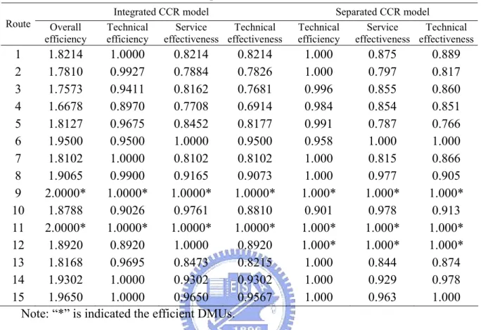
Constant returns to scaleIn this part, we use individual model to develop an integrated CCR model (ICCR). We let each model decide its multiplier in the integrated model at the same time. Technical efficiency stands for production sector and service effectiveness represents sale sector; however, technical effectiveness doesn’t stand for any sector as non-storable commodities are produced. That’s why this study doesn’t employ technical effectiveness to evaluate the performance.
w v u Max , , ⎟⎟ ⎟ ⎟ ⎟ ⎠ ⎞ ⎜⎜ ⎜ ⎜ ⎜ ⎝ ⎛ + ⎟⎟ ⎟ ⎟ ⎟ ⎠ ⎞ ⎜⎜ ⎜ ⎜ ⎜ ⎝ ⎛
∑
∑
∑
∑
= = = = s r kr r p q kq q m j kj j s r kr r y u l w x v y u 1 1 1 1 (2-7) s.t.∑
∑
= = ≤ m j ij j s r ir ry v x u 1 1 , i=1 L,2, ,n∑
∑
= = ≤ s r ir r p q iq ql u y w 1 1 , i=1 L,2, ,n0 ≥ j v , j=1 L,2, ,m 0 ≥ q w , q=1 L,2, ,p 0 ≥ r u , r =1 L,2, ,s
Once we proposed the original model, we can add slack analysis in this model. In order to do slack analysis, we add slack variables in each variable. The ICCR model shows as following and ICCR model assumes production and sale sector is equal weight.
w v u Max , , ⎟⎟ ⎟ ⎟ ⎟ ⎠ ⎞ ⎜⎜ ⎜ ⎜ ⎜ ⎝ ⎛ + ⎟⎟ ⎟ ⎟ ⎟ ⎠ ⎞ ⎜⎜ ⎜ ⎜ ⎜ ⎝ ⎛
∑
∑
∑
∑
= = = = s r kr r p q kq q m j kj j s r kr r y u l w x v y u 1 1 1 1 (2-8) s.t.∑
∑
(
)
= = − ≤ m j kj kj j s r ir ry v x s u 1 1 , i=1 L,2, ,n(
)
∑
∑
= = ≤ + s r ir r p q kq kq q l s u y w 1 1 , i=1 L,2, ,n 0 ≥ j v , j=1 L,2, ,m 0 ≥ q w , q=1 L,2, ,p 0 ≥ r u , r =1 L,2, ,sIn the revised model, we hold production variable ( y ) ir unchanged. That means we only have to minimize the input and maximize the service value. In other words, there wouldn’t be slack value of production variable. Through this model, we can get the performance value and slack variable.
Then we can rewrite this model as following:
⎟⎟ ⎠ ⎞ ⎜⎜ ⎝ ⎛ ⎟⎟ ⎠ ⎞ ⎜⎜ ⎝ ⎛ + ⎟ ⎠ ⎞ ⎜ ⎝ ⎛ ⎟ ⎠ ⎞ ⎜ ⎝ ⎛ =
∑
∑
∑
∑
= = = = m j kj j p q kq q s r kr r s r kr ry u y w l v x u h 1 1 1 1 w v uMax
, ,s.t. 1 1 1 = ⎟ ⎠ ⎞ ⎜ ⎝ ⎛ ⎟⎟ ⎠ ⎞ ⎜⎜ ⎝ ⎛
∑
∑
= = s r ir r m j ij jx u y v (2-9)(
)
∑
∑
= = − ≤ m j kj kj j s r ir ry v x s u 1 1 , i=1 L,2, ,n(
)
∑
∑
= = ≤ + s r ir r p q kq kq q l s u y w 1 1 , i=1 L,2, ,n 0 ≥ j v , j=1 L,2, ,m 0 ≥ q w , q=1 L,2, ,p 0 ≥ r u , r =1 L,2, ,sWe can use this integrated model to calculate the value of cost efficiency and service effectiveness for each DMU. Then we would know which DMU has the best performance and how does it improve its performance. This IDEA model cannot transfer to dual form, because IDEA model isn’t the linear programming problem.
In eg. 2-8, h stands for the overall efficiency score, which is the efficiency of kth firm, and it ranges from zero to two. If h equals to two, the firm is efficient. And if h is less two, the firm is inefficient. If firm is inefficiency, one can check the efficiency scores, which respectively calculated from the integrated model (cost efficiency, service effectiveness and cost effectiveness) to see which part need to improve.
3.2.1.3.2.
Variable returns to scaleIn order to fit the true production behavior, we are going to change CRS production technique into VRS production technique. Because our model form is a nonlinear problem, we can not use conventional way to add VRS variable (
∑
λ=1) in dual problem. We add our VRS variable in following BCC model (IBCC).w v u Max , , ⎟⎟ ⎟ ⎟ ⎟ ⎠ ⎞ ⎜⎜ ⎜ ⎜ ⎜ ⎝ ⎛ − − + ⎟⎟ ⎟ ⎟ ⎟ ⎠ ⎞ ⎜⎜ ⎜ ⎜ ⎜ ⎝ ⎛ −
∑
∑
∑
∑
= = = = 0 1 1 1 1 0 1 u y u u l w x v u y u s r kr r p q kq q m j kj j s r kr r (2-10) s.t.∑
∑
(
)
= = − ≤ − m j kj kj j s r ir ry u v x s u 1 0 1 , i=1 L,2, ,n(
)
0 1 1 1 u y u u s l w s r ir r p q kq kq q + − ≤∑
−∑
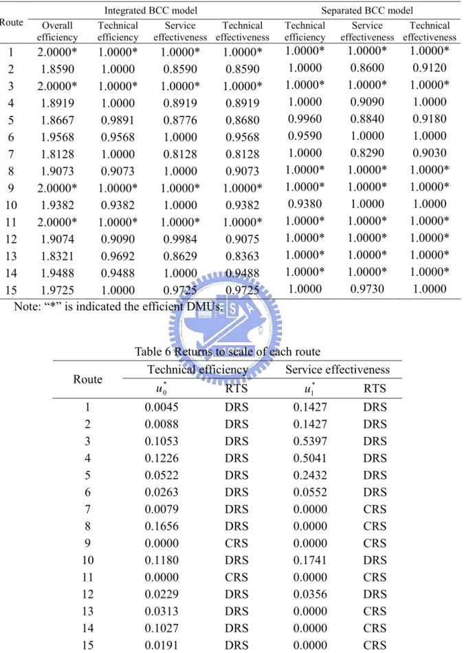
= = , i=1 L,2, ,n 0 ≥ j v , j=1 L,2, ,m 0 ≥ q w , q=1 L,2, ,p 0 ≥ r u , r =1 L,2, ,sWe can use this model to get the performance value of each DMU under VRS technique. From this proposed model we can get efficiency value, slack value and we also can know each DMU is in increase, decrease or constant returns to scale.
4. Properties of the proposed IDEA Models
In this chapter, we prove that the proposed IDEA models exhibits two essential properties: rationality and uniqueness.
4.1. Rationality
4.1.1.
Rationality for ICCR modelAccording to Charnes, et al. (1978), their proposed measure of the efficiency of any DMU is obtained as the maximum of a ratio of weighted outputs, subject to the condition that the similar ratio for every DMU be less than or equal to unity. Since the proposed integrated DEA model is to maximize two aspects of efficiency values, the overall efficiency value should be less than or equal to two. Our proposed measure of the efficiency of any DMU can also be obtained in a similar way. Mathematically,
[ICCR’] w v u Max , , ⎟ ⎟ ⎟ ⎟ ⎠ ⎞ ⎜ ⎜ ⎜ ⎜ ⎝ ⎛ + ⎟⎟ ⎟ ⎟ ⎟ ⎠ ⎞ ⎜⎜ ⎜ ⎜ ⎜ ⎝ ⎛
∑
∑
∑
∑
= = = = R r kr r S s ks s J j kj j R r kr r y u l w x v y u 1 1 1 1 st. 1 1 1 ≤∑
∑
= = J j ij j R r ir r x v y u , i=1 L,2, ,I 1 1 1 ≤∑
∑
= = R r ir r S s is s y u l w , i=1 L,2, ,I 0 ≥ j v , j=1 L,2, ,J 0 ≥ s w , s=1 L,2, ,S 0 ≥ r u , r=1 L,2, ,R Let r R r x x E′ = and R r r l lE′′= respectively represent the technical
efficiency (ratios of inputs at a given output) and service effectiveness (ratios of consumptions at a given output), where x is the minimum input that can R
produce the given output and x is the actual input being rated from the r same output. Likewise, l is the maximum yield that can be generated from R
the given output and l is the actual yield being rated from the same output. r Then, the overall efficiency can be calculated as
R r r R r r r l l x x E E E = ′ + ′′= + .
Essentially, 20≤Er ≤ .
Alternately, we can also derive the overall efficiency, E , from our r proposal integrated DEA model as follows. For any given output y,
v u Max , r r r r r uy wl vx uy h = + s.t. ≤1 R R vx uy , 1 ≤ r r vx uy , 1 ≤ R R uy wl , 1 ≤ r r uy wl , u , v ,w≥0
Let u*,v*, w*represent the optimal pair of corresponding values. Since r R x x ≤ , lR ≥lr and yR = yr = y , it implies u yr u yR v xR * * * = = and R R r u y w l y
u* = * = * . We then have the following results and relationship:
Technical efficiency= r r R r R r r E x v x v x v y u x v y u = = = ′ * * * * * * Service effectiveness= r R r R r r r E l w l w y u l w y u l w = = = ′′ * * * * * * Thus, r r r r o y u l w x v y u h * * * * + = =Er′ +Er′′=Er.
In conclusion, the efficiency scores determined by the proposed integrated DEA model are proven with an essential property of reasonability because the optimal values of the proposed model have satisfied the definition of efficiency.
4.1.2.
Rationality for IBCC model[IBCC’] w v u Max , , ⎟ ⎟ ⎟ ⎟ ⎠ ⎞ ⎜ ⎜ ⎜ ⎜ ⎝ ⎛ − − + ⎟⎟ ⎟ ⎟ ⎟ ⎠ ⎞ ⎜⎜ ⎜ ⎜ ⎜ ⎝ ⎛ −
∑
∑
∑
∑
= = = = R r kr r S s ks s J j kj j R r kr r u y u u l w x v u y u 1 0 1 1 1 1 0 s.t. 1 1 1 0 ≤ −∑
∑
= = J j ij j R r ir r x v u y u , i=1 L,2, ,I 1 1 0 1 1 ≤ − −∑
∑
= = R r ir r S s is s u y u u l w , i=1 L,2, ,I vj ≥0, j=1 L,2, ,J ws ≥0, s=1 L,2, ,S ur ≥0, r=1 L,2, ,RThe definition of efficiency is the same as in ICCR model. We can derive the overall efficiency from our proposal integrated DEA model as follows.
v u Max , 0 1 0 u uy u wl vx u uy h r r r r r − − + − = s.t. − 0 ≤1 R R vx u uy , 1 0 ≤ − r r vx u uy , 1 0 1 ≤ − − u uy u wl R R , 1 0 1 ≤ − − u uy u wl r r , u , v ,w≥0 Let *
u ,v*, w*, u*0, u represent the optimal pair of corresponding 1*
values. Since xR ≤xr , lR ≥lr and yR = yr = y , it implies
R R
r u u y u v x
y
u* − 0 = * − 0 = * and u*yr −u0 =u*yR −u0 =w*lR −u1. We then have the following results and relationship:
Technical efficiency = r r R r R r r E x v x v x v u y u x v u y u ′ = = − = − * * * 0 * * 0 *
Service effectiveness 1 * 1 * 0 * 1 * 0 * 1 * u l w u l w u y u u l w u y u u l w R r R r r r − − = − − = − − = * 1 * 1 * 1 * * 1 *
)
(
)
(
w
u
l
w
u
l
w
u
l
w
w
u
l
w
R r R r−
−
=
−
−
=
0 <Service effectiveness= E w u l w u l R r ~ * 1 * 1 = − − <1,Where u is a scale variable. 1
When 0u1> , we can get the result: 1* w
u l
lr > r − . That means DMU r needs to downsize. Then it can reach optimal scale.
When 0u1= , we can get the result: 1* w u l
lr = r − . That means DMU r reaches optimal scale.
When 0u1< , we can get the result: 1* w u l
lr < r − . That means DMU r needs to upsize. Then it can reach optimal scale.
In conclusion, the efficiency scores determined by the proposed integrated DEA model are proven with an essential property of rationality. Furthermore, IBBC model can determine the optimal scale of each DMU.
4.2. Uniqueness
To show the uniqueness of joint efficiency measurement of the proposed model, we have to prove that the virtual multipliers of u, v, and w determined by the proposed model are a global optimal solution, not a local one. For a nonlinear programming problem, only for the model with a convex or concave objective function under a convex feasible region (i.e. sufficient conditions) would the solutions, obtained via the Karush-Kuhn-Tucker (KKT) conditions (i.e. necessary conditions), guarantee a global optimum. In other words, the convexity or concavity of objective function together with the convexity of feasible region must be examined. For simplicity, without loss of generality, the mathematical model of [ICCR-S] and [IBCC-S] are examined and only the case of single input, output and service variable is presented.
Since all the constraints in [ICCR-S] and [IBCC-S] are linear, the feasible set defined by these constraints is convex. Then the bordered Hessian matrix of
objective function of [ICCR-S] can be computed as: w lu y yv x lu y yv x u yv x lu y H 3 1 2 1 2 1 2 1 3 1 2 1 2 2 0 0 0 − − − − − − − − − − − − − − − − =
The signs of the first, second and third leading principal minors of H are 0
1 ≤
H , H2 ≥0and H3 ≤0 indicating that the bordered Hessian is negative
semi-definite and the objective function is a concave function. In other words, the sufficient conditions for a global maximum are proven.
The bordered Hessian matrix of objective function of [IBCC-S] can be computed as: = H
(
)
(
)
(
)
( )
( )
(
)
(
)
(
)
( )
(
)
(
)(
)
(
)(
)
(
)
( )
(
)
(
)(
)
(
)(
)
3 0 1 2 3 0 1 2 0 2 2 0 3 0 1 3 0 1 2 0 2 2 0 2 0 2 0 2 2 0 3 1 2 0 2 0 2 2 2 2 0 0 0 0 2 0 0 0 0 − − − − − − − − − − − − − − − − − − − − − − − − − − − − − − − − − − − − − − − − − − − u uy u wl y u uy u wl y u uy y vx xy u uy yl u uy u wl y u uy u wl u uy vx x u uy l u uy y u uy vx xy vx x u uy v x u uy yl u uy lThe signs of principal minors of H are H1 ≤0, H2 ≥0, H3 ≤0,
0
4 ≥
H and H5 ≤0. This indicating that the bordered Hessian is negative
semi-definite and the objective function is a concave function. In other words, the sufficient conditions for a global maximum are proven.