最小化線性退化性工件總完工時間之 單機一次維修排程問題

國立交通大學

工業工程與管理學系

碩士論文

最小化線性退化性工件總完工時間之

單機一次維修排程問題

Scheduling Linear Deteriorating Jobs on a Single

Machine with a Rate-modifying Activity to Minimize

Flow Time

研究生

：

楊承翰

指導教授

：

許錫美 博士

洪暉智 博士

最小化線性退化性工件總完工時間之

單機一次維修排程問題

Scheduling Linear Deteriorating Jobs on a Single Machine with a

Rate-modifying Activity to Minimize Flow Time

研究生：楊承翰 Student: Cheng-Han Yang

指導教授：許錫美 博士 Advisor: Dr. Hsi-mei Hsu

國立交通大學

工業工程與管理學系

碩士論文

A Thesis

Submitted to Department of Industrial Engineering and Management

College of Management

National Chiao Tung University

in Partial Fulfillment of the Requirements

for the Degree of

Master

in

Industrial Engineering

June 2013

Hsin-Chu, Taiwan, Republic of China

中 華 民 國 一 百 零 二 年 六 月

Dr. Hui-chih Hung

洪暉智 博士

i

最小化線性退化性工件總完工時間之

單機一次維修排程問題

研究生:楊承翰 指導教授:許錫美 博士

洪暉智 博士

國立交通大學工業工程與管理學系碩士班

摘要

ii

Scheduling Linear Deteriorating Jobs on a Single Machine with a

Rate-modifying Activity to Minimize Flow Time

Student: Cheng-Han Yang Advisor: Dr. Hsi-Mei Hsu Dr. Hui-Chih Hung

Department of Industrial Engineering and Management National Chiao Tung University

Abstract

Consider a scheduling problem with deteriorating jobs and single rate-modify activity on a single machine, we attempt to determine the job sequence and RMA position for minimizing the flow time. We first show that the problem is NP-complete. Then, we explore several important properties for the optimal solutions. We find that the coefficients of the objective function are the key factor to determine the value of flow time and purpose a heuristic on those properties. Numerical studies are implemented to verify the efficiency of the proposed heuristic.

iii

Contents

1.1 Research background and motivation. ... 1

1.2 Research scopes ... 3

Chapter 2. Literature Reviews ... 4

2.1 Deteriorating jobs... 4

2.2 Optimal scheduling properties ... 5

2.3 Rate-modifying activity ... 5

Chapter 3. Problem formulation ... 7

3.1 Problem definition ... 7

3.2 Assumptions ... 8

3.3 Notations ... 8

3.4 Formulation ... 9

Chapter 4. Properties and solution approaches ... 11

4.1 Problem complexity ... 11

4.2 Optimality properties ... 11

4.3 Solutions approach ... 15

Chapter 5. Experiment design and numerical study ... 22

5.1 Generating of experiment data ... 22

5.2 Experiment results ... 22

Chapter 6. Conclusions and future researches ... 27

iv

Table Contents

Table 1. Coefficients for , and for 4 job example. ... 16

Table 2. Deteriorating rates of a 10 job example. ... 17

Table 3. Coefficients for , and for a 10 job example. ... 18

Table 4. and for Subroutine Improvement Two ... 21

Table 5. Relative errors for α~U 0,1 ,α~U 0,3 ,α~U 0,5 and α~U 0,10 ... 23

Table 6. Relative errors for α~U 0,20 ,α~U 0,30 and α~U 0,40 ... 24

Table 7. Relative errors for α~U 10,40 ,α~U 20,40 and α~U 30,40 ... 25

v

Figure Contents

Figure 1. Research scopes. ... 3 Figure 2. Problem scopes ... 7 Figure 3. Computational times ... 26

1

Chapter 1. Introduction

We first introduce the background and motivation of this study. Then, we show the research structure.

1.1 Research background and motivation.

Most previous scheduling research has focused on problems with a standard set of assumptions. One of these assumptions is that processing times of the jobs are constant, but this is not proper for some real life situations. In reality, the processing time of a job may be variable. The processing time of a job may be influenced by various factors. The scheduling problem with varying processing times has received increasing attention in recent years.

Generally, there are two types of problems with varying processing time. One is varying from time, which is called the time-dependent processing times, and the other is varying from position, which is called the position-dependent processing times. In our study, we consider the time-dependent processing times only.

Actually, there are two kinds of time-dependent processing times, the first kind of time-dependent processing times is called learning effect. This learning effect leads to a result that the later of job being processed, the shorter of its processing time to be required. The second kind is called deteriorating effect. The processing time of a job is characterized as a non-decreasing function of its start time to be processed. For the deteriorating effect, a job which is processed later in time has a longer processing time. In our study, this deteriorating effect is what we primarily focus on.

For example, ion implantation is a process used in semiconductor and materials science research. In semiconductor, implantation is used to changing the surface properties and electrical characteristics of the wafer. Implantation equipment includes an ion source, an

2

accelerator and a target chamber. Ion source generate an ion beam and be accelerated in electrical field, then implant the ions to the wafer. During the implantation, the processing time increases due to the decreasing of the ion beam, and this phenomenon is called deteriorating. In order to find a way of dealing with this difficulty, a mechanism called rate-modify activity (RMA) occurred.

The problems mentioned above have led to a number of discussions recently. A rate-modify activity (RMA) is an activity that changes the production rate of the equipment or machine under some considerations. In our study, RMA is defined as a maintenance activity and the machine is not available during its being maintained. The status of a machine after RMA is assumed to return to its initial state.

This study considers the scheduling deteriorating jobs on a signal machine with a rate-modify activity (RMA). We attempt to determine the job sequence and the RMA position for minimizing jobs flow time.

3

1.2 Research scopes

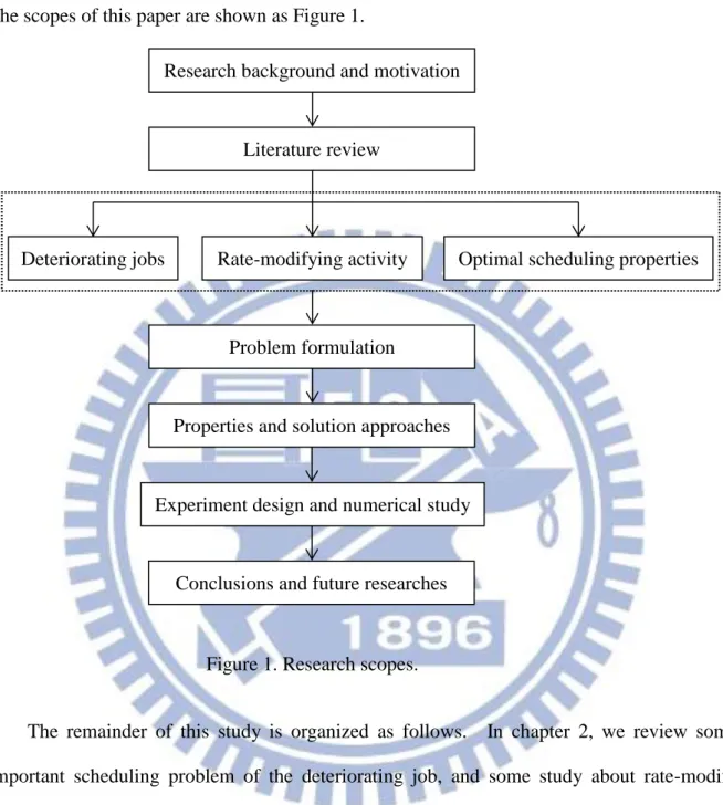
The scopes of this paper are shown as Figure 1.

Figure 1. Research scopes.

The remainder of this study is organized as follows. In chapter 2, we review some important scheduling problem of the deteriorating job, and some study about rate-modify activity. In chapter 3, we first define our problem and show the assumptions and notations used in this study. Then, our problem is formulated as a mathematical programming mode. In chapter 4, we prove some important properties and develop our heuristic. In chapter 5, we do experiment design and numerical study. Finally, the conclusions and future works are presented in the last section.

Problem formulation

Properties and solution approaches Research background and motivation

Literature review

Deteriorating jobs Rate-modifying activity Optimal scheduling properties

Experiment design and numerical study

4

Chapter 2. Literature Reviews

Literature related to our study focus arises on deteriorating jobs, the optimal scheduling properties and rate-modifying activity.

2.1 Deteriorating jobs

Gupta and Gupta (1988) introduced a scheduling model to determine the job sequence. The objective is to minimize the makespan where the processing times of jobs are described as a monotonically increasing function of their starting time. They proposed an effective heuristic for a nonlinear deteriorating function. Browne and Yechiali (1990) was the first one who defined the phenomenon of deterioration in processing time described by Gupta and Gupta (1988) as deteriorating jobs. They assumed that the processing time of job increases linearly based on its starting time. Under this assumption, they presented optimal scheduling polices to minimize the makespan for n jobs on a single machine. Mosheiov (1991) considered a problem with flow time minimization where the complexity is higher than the problem with makespan minimization. He modified the deteriorating function of Browne and Yechiali (1990) with an identical basic processing time to reduce the complexity. He proposed several important properties relating to the optimal policy. Mosheiov (1994) further simplified the model to a simple linear deteriorating function and observed a fact that the makespan won’t be affected by the sequence of jobs. Furthermore, Mosheiov (1995) considered piecewise linear deteriorating functions and showed that this is a NP-complete problem. He formulated this problem as an integer programming model. He proposed an algorithm and illustrates a lot of numerical examples to show the accurate and efficient of the algorithm. Bachman et al. (2002) showed that minimizing the weighted flow time is a NP complete problem. Mosheiov (2002) considered different production scenarios such as job shop, flow shop and open shop for minimizing the makespan of n jobs on multiple machines.

5

After that, Mosheiov (2005) studied a different type of function which based on exponentially deteriorating of its position, and purposed some important properties to minimize flow time.

2.2 Optimal scheduling properties

Brown and Yechiali (1990) study a scheduling problem to minimize makespan. They assumed that a job’s actual processing time can be described as a linear function of its starting time𝑝_𝑗+ 𝛼_𝑗𝑠_𝑗, where 𝑝_𝑗 is a job’s basic processing time, 𝛼_𝑗 is the job’s deteriorating rate, and 𝑠_𝑗 is the job’s starting time. In their study, they proved that to schedule jobs in a non-decreasing order of the ratio 𝑝_𝑗⁄ 𝛼_𝑗 is an optimal policy. Mosheiov (1991) consider the deteriorating problem of minimizing the flow time of jobs with an identical basic processing time and different deteriorating rates. He proved that the optimal sequence of jobs must satisfy a V-shape. They defined V-shape as “jobs are arranged in descending order of growth rate if they are placed before the minimal growth rate job, and in ascending order if placed after it.” This paper is a very important reference for our study.

Some researchers considered the situations of a scheduling problem where the processing time of a job is an increasing function of its position in the sequence. Mosheiov (2005) studied a scheduling problem to minimize flow time with exponentially deteriorating function which could be described as 𝑝_{𝑗 𝑗}𝛼 (𝛼 > 0), where 𝑝_𝑗 is a job’s basic processing time, 𝑗 is the job’s position, and 𝛼 is a constant which describes the deteriorating rate.

And the author showed that an optimal schedule is V-shaped with respect to job’s processing time.

2.3 Rate-modifying activity

Rate-modifying activity (RMA) is an issue appeared recently and first introduced by Leo and Leon (2001). Motivated by a problem found in electronic assembly lines, they defined

6

RMA as an activity that changes the production rate of the equipment under consideration. The decisions are when to schedule the RMA and the sequence of jobs under different objectives. They also developed polynomial time algorithms and a pseudo-polynomial time algorithm for various performance measures. Lee and Lin (2001) considered the problems involving repair and maintenance activities which they also called RMA. They studied two types of processing cases, resumable and nonresumable. The resumable job is defined as follows: Once the job is interrupted during it been processed, the job can keep processing after interruption. On the other hand, if the job could not continue its processing after interruption, these jobs are called nonresumable job. The objective functions in their paper are makespan minimization, flow time minimization and maximum lateness minimization respectively. Zhao et al. (2009) considered the two-parallel machines scheduling problem with RMA. They provided polynomial and pseudo-polynomial time algorithms to solve the weighted flow time minimization problem. Ozturkoglu and Bulfin (2010) considered the problem with the job sequence, the number of RMAs and RMA positions. They formulated integer programming models to solve makespan and flow time minimization problems. They also proposed efficient heuristic algorithms for solving large size problems. Lodree and Geiger (2010) studied the scheduling problem to minimize makespan with both time-dependent processing time and RMA. They show that the optimal policy is to schedule the RMA in the middle of the task sequence under certain conditions.

7

Chapter 3. Problem formulation

We first define our problem and show the assumptions and notations used in thisstudy. Then, our problem is formulated as a mathematical programming model.

3.1 Problem definition

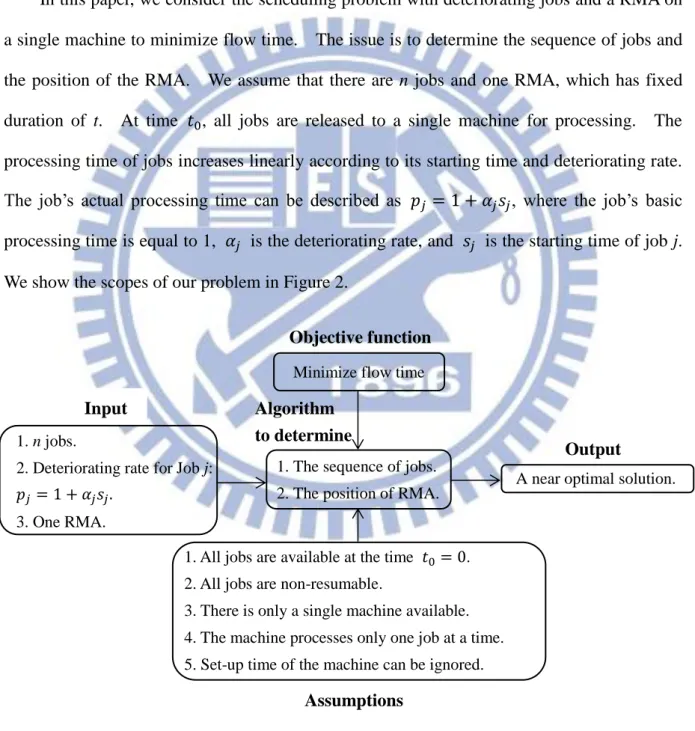
In this paper, we consider the scheduling problem with deteriorating jobs and a RMA on a single machine to minimize flow time. The issue is to determine the sequence of jobs and the position of the RMA. We assume that there are n jobs and one RMA, which has fixed duration of t. At time 𝑡 , all jobs are released to a single machine for processing. The processing time of jobs increases linearly according to its starting time and deteriorating rate. The job’s actual processing time can be described as 𝑝𝑗 = 1 + 𝛼𝑗𝑠𝑗, where the job’s basic

processing time is equal to 1, 𝛼_𝑗 is the deteriorating rate, and 𝑠_𝑗 is the starting time of job j. We show the scopes of our problem in Figure 2.

Figure 2. Problem scopes

Minimize flow time

Objective function

A near optimal solution.

Output Algorithm

to determine

1. The sequence of jobs. 2. The position of RMA. 𝑝_𝑗= 1 + 𝛼_𝑗𝑠_𝑗.

1. n jobs.

2. Deteriorating rate for Job j:

3. One RMA.

Input

Assumptions

1. All jobs are available at the time 𝑡 = 0. 2. All jobs are non-resumable.

3. There is only a single machine available. 4. The machine processes only one job at a time. 5. Set-up time of the machine can be ignored.

8

3.2 Assumptions

There are some assumptions used in this paper. 1. All jobs are available at the time 𝑡 = 0.

2. All jobs are non-resumable. That is, any job being processed should not be interrupted or separated.

3. There is only a single machine available. 4. The machine processes only one job at a time.

5. Set-up time of the machine can be ignored. That is, when the machine’s RMA is finished, jobs can be processed immediately.

3.3 Notations

Now we define the notations for formulating our mathematical model. 𝑁 : The set of jobs, where 𝑁 = {1,2, … , 𝑛} and |𝑁| = 𝑛.

𝑗 : The index of jobs, where 𝑗 𝑁. 𝑠_𝑗 : The starting time of Job 𝑗, for 𝑗 𝑁.

𝛼𝑗 : The deteriorating rate of Job 𝑗, for 𝑗 𝑁. Note that 𝛽𝑗 = 1 + 𝛼𝑗.

𝑝_𝑗 : The actual processing time of Job 𝑗, where 𝑝𝑗 = 1 + 𝛼𝑗𝑠𝑗, for 𝑗 𝑁.

𝐶𝑗 : The completion time of Job 𝑗, for 𝑗 𝑁.

𝐾 : The set of jobs arranged before RMA, where |𝐾| = 𝑘. Note that 𝑁\𝐾 is the set of jobs arranged after RMA.

𝑡 : The fixed duration of RMA.

𝜋 : A sequence of n jobs, where 𝜋 = 𝜋 , 𝜋 , … , 𝜋 and 𝜋 is the r-th job in 𝜋.

𝜋𝑘∗ _{: The optimal sequence of 𝑛 jobs subject to exact 𝑘 jobs arranged before}

9

𝐼 𝜋 : The inverse sequence of 𝜋. Note that 𝐼 𝜋 = 𝜋 , … , 𝜋 , 𝜋 , for 𝜋 = 𝜋 , 𝜋 , … , 𝜋 .

𝐶_𝑘 : The terms in the objective function with 𝛽 subject to exact 𝑘 jobs arranged before RMA.

𝑘 = 𝐶𝑘 /𝛽 .

3.4 Formulation

There are n deteriorating jobs and one RMA to be scheduled on a single machine. The processing times of jobs increase linearly based on its starting time and the actual processing time can be defined as 𝑝_𝑗 = 1 + 𝛼_𝑗𝑠_𝑗. Given a schedule 𝜋 = 𝜋 , 𝜋 , … , 𝜋 , where 𝜋 is the th job in 𝜋. We assume that all jobs are available at the time 𝑡 = 0. For the schedule 𝜋, Jobs 𝜋 , 𝜋 , … , 𝜋_𝑘 are arranged before RMA and Jobs 𝜋_𝑘+ , 𝜋_𝑘+ , … , 𝜋 are arranged after RMA.

First, we consider the jobs before RMA. The actual processing time for 𝜋 is 𝑝_𝜋1 = 1 and the completion time for 𝜋 is 𝐶_𝜋1 = 1. For those jobs before RMA, the completion time for 𝜋 is

where 𝛽_𝜋𝑠 = 1 + 𝛼_𝜋𝑠.

Then, we consider the jobs after RMA. The actual processing time for 𝜋_𝑘+ is 𝑝_𝜋𝑘+1 = 1 and the completion time for 𝜋_𝑘+ is

For those jobs after RMA, the completion time for 𝜋 is

𝐶𝜋𝑟 = 𝛽𝜋𝑠 𝑘 𝑠=𝑖+ 𝑘 𝑖= + 𝑡 + 𝛽𝜋𝑠 𝑟 𝑠=𝑖+ 𝑟 𝑖=𝑘+ , for 𝑟 = 𝑘 + 1, 𝑘 + 2, … , 𝑛. (3.2) (3.1) 𝐶𝜋𝑟 = 𝛽𝜋𝑠 𝑟 𝑠=𝑖+ 𝑟 𝑖= , , for 𝑟 = 1,2, … , 𝑘, 𝐶𝜋𝑘+1 = 𝐶𝜋𝑘+ 𝑡 + 𝑝𝜋𝑘+1 = 𝛽𝜋𝑠 𝑘 =𝑖+ 𝑘 𝑖= + 𝑡 + 1.

10

By Equation (3.1) and (3.2), for given schedule 𝜋 and RMA position k, the flow time Z 𝜋, 𝑘 is

Our objective is to minimize flow time. Therefore, we can formulate our problem as follows:

For 𝑁 ⊆ 𝑁 and |𝑁 | = n − 𝑘, 𝜋 represents an arbitrary permutation of 𝑁 . If we consider the problem after RMA, we can formulate the Subproblem B as follows:

𝑍 𝜋, 𝑘 = 𝛽𝜋𝑠 ℎ =𝑖+ + 𝑛 − 𝑘 𝛽𝜋𝑠 𝑘 =𝑖+ 𝑘 𝑖= + 𝑡 ℎ 𝑖= 𝑘 ℎ= + 𝛽𝜋𝑠 ℎ =𝑖+ ℎ 𝑖=𝑘+ ℎ=𝑘+ . min 𝜋,𝑘 𝑍 𝜋, 𝑘 s.t. 𝑍 𝜋, 𝑘 = 𝛽_𝜋𝑠 ℎ 𝑠=𝑖+ + 𝑛 − 𝑘 𝛽𝜋𝑠 𝑘 𝑠=𝑖+ 𝑘 𝑖= + 𝑡 ℎ 𝑖= 𝑘 ℎ= 𝑘 = 1,2, … , 𝑛 − 1. (A) min 𝜋0 𝑍 𝜋 s.t. 𝑍 𝜋 = 𝛽_𝜋 𝑠0 ℎ 𝑠= 𝑛−𝑘 ℎ= (B)

11

Chapter 4. Properties and solution approaches

In this chapter, we first show the complexity of our problem, and then prove some important properties. We also propose a heuristic based on those properties.

4.1 Problem complexity

One of the special cases 𝑘 = 0 of our problem is the same as the problem considered by Mosheiov (1991). Moreover, Mosheiov have proved that his problem is NP-complete and the complexity of his problem is O 2 . Therefore, our problem is NP-complete.

In order to solve our problem, we have to explore some important properties and develop a heuristic based on those properties.

4.2 Optimality properties

We first show that the jobs with the largest and the second largest deteriorating rates should be placed at the first positions or the positions right after the RMA.

Property 1. Consider Problem A with given k jobs arranged before RMA. We have 𝛽_𝜋

ℎ 𝑘∗ ≥ 𝛽_𝜋

𝑞

𝑘∗, for ℎ = 1 𝑜 𝑘 + 1 𝑎𝑛𝑑 𝑜 𝑞 𝑁\{1, 𝑘 + 1}.

Proof. Suppose we have a sequence 𝜋𝑘∗ = (𝜋𝑘∗, 𝜋𝑘∗, … , 𝜋𝑘∗), where 𝛽_𝜋

1 𝑘∗ < 𝛽_𝜋

𝑞 𝑘∗ for

some 𝑞 𝑁\{1, 𝑘 + 1}. We have an interchange between positions 1 and q which called sequence 𝜋′. That is 𝜋′ = 𝜋′, 𝜋′, … , 𝜋′ , where 𝜋′ = 𝜋𝑞𝑘∗, 𝜋𝑞′ = 𝜋𝑘∗, and 𝜋𝑖′ = 𝜋𝑖𝑘∗, for

12

From Problem A, we have

where the above inequality holds because 𝛽_𝜋𝑞′ = 𝛽_𝜋 1 𝑘∗ < 𝛽_𝜋

𝑞

𝑘∗. Thus, 𝜋𝑘∗ will never be

optimal. Contradiction.

Similarly, 𝛽_𝜋

ℎ𝑘∗ ≥ 𝛽𝜋𝑞𝑘∗, for ℎ = 𝑘 + 1 and 𝑞 𝑁\{1, 𝑘 + 1}. ∎

Property 2. Consider Problem A with given k jobs arranged before RMA. Define 𝜋 = 𝜋 , 𝜎 , 𝜋_𝑘+ , 𝜎 and 𝜋′_{= 𝜋 , 𝜎 , 𝜋}

𝑘+ , 𝐼 𝜎 , where 𝜎 = 𝜋 , 𝜋 , … , 𝜋𝑘 and

𝜎 = 𝜋𝑘+ , 𝜋𝑘+ , … , 𝜋 . We have 𝑍 𝜋 = 𝑍 𝜋′ .

Proof. From Problem A with given k jobs arranged before RMA, we can derived as follow 𝑍 𝜋 − 𝑍 𝜋′ = 𝛽_𝜋𝑠 ℎ =𝑖+ ℎ 𝑖=𝑘+ ℎ=𝑘+ − 𝛽_𝜋𝑠′ ℎ =𝑖+ ℎ 𝑖=𝑘+ ℎ=𝑘+ = (1 + 𝜋𝛽𝑘+2) + (1 + 𝜋𝛽𝑘+2𝜋𝛽𝑘+3+ 𝜋𝛽𝑘+3) + ⋯ +(1 + 𝜋_𝛽𝑘+2… 𝜋_𝛽𝑛−1 + ⋯ + 𝜋_𝛽𝑛−1) + 1 + 𝜋_𝛽𝑘+2… 𝜋_𝛽𝑛−1𝜋_𝛽𝑛 + ⋯ + 𝜋_𝛽𝑛−1𝜋_𝛽𝑛+ 𝜋_𝛽𝑛 −[ 1 + 𝜋_𝛽𝑛 + 1 + 𝜋_𝛽𝑛𝜋_𝛽𝑛−1 + 𝜋_𝛽𝑛−1 + ⋯ + 1 + 𝜋_𝛽𝑛… 𝜋_𝛽𝑘+3+ ⋯ + 𝜋_𝛽𝑘+3 + 1 + 𝜋_𝛽𝑘+2… 𝜋_𝛽𝑛−1𝜋_𝛽𝑛 + ⋯ + 𝜋_𝛽𝑛−1𝜋_𝛽𝑛+ 𝜋_𝛽𝑛 ] = 0. = (

𝛽

𝛽

𝛽

𝛽

𝛽

𝛽

13

Consequently, 𝑍 𝜋 = 𝑍 𝜋′ . ∎

Property 3. Consider Problem A with given k jobs arranged before RMA. We have 𝛽_𝜋

ℎ 𝑘∗ ≥ 𝛽_𝜋

𝑞

𝑘∗, for ℎ = 𝑘 + 2 or 𝑛 and for some 𝑞 {𝑘 + 3, 𝑘 + 4, … , 𝑛 − 1}.

Proof. Suppose we have a sequence 𝜋𝑘∗ = 𝜋𝑘∗, 𝜋𝑘∗, … , 𝜋𝑘∗ , where 𝛽_𝜋

𝑘+2 𝑘∗ < 𝛽_𝜋

𝑞 𝑘∗ for

all 𝑞 {𝑘 + 3, 𝑘 + 4, … , 𝑛 − 1}. Then, we interchange 𝜋_𝑘+ 𝑘∗ and 𝜋_𝑘+ 𝑘∗ which called sequence 𝜋′. That is 𝜋′= 𝜋′, 𝜋′… , 𝜋′ , where 𝜋_𝑘+ ′ = 𝜋_𝑘+ 𝑘∗ , 𝜋_𝑘+ ′ = 𝜋_𝑘+ 𝑘∗ .

From Problem A, we have

where 𝛽_𝜋 𝑖 𝑘∗ ≥ 1 , for 𝑖 = 1,2, … , 𝑛 and 𝛽_𝜋 𝑘+2 𝑘∗ ≤ 𝛽_𝜋 𝑘+3

𝑘∗ . The above expression is

nonpositive. Thus, 𝜋𝑘∗ will never be optimal. Contradiction. Similarly, 𝛽_𝜋

ℎ𝑘∗ ≥ 𝛽𝜋𝑞𝑘∗, for ℎ = 𝑛 and for some 𝑞 𝑁\{1, 𝑘 + 1}. ∎

Property 4. Consider Problem A with given k jobs arranged before RMA. Let 𝑖 − 1, i, i+1 be three consecutive positions in a sequence and 𝑖 + 1 ≤ 𝑘. If 𝛽_𝜋

𝑖 𝑘∗ > 𝛽_𝜋 𝑖−1𝑘∗ and 𝛽_𝜋 𝑖 𝑘∗ > 𝛽_𝜋 𝑖+1

𝑘∗ , then 𝜋𝑘∗ is not optimal.

Proof. Suppose we have a sequence 𝜋𝑘∗ = 𝜋𝑘∗, 𝜋𝑘∗, … , 𝜋𝑘∗ where 𝛽_𝜋

𝑖 𝑘∗ > 𝛽_𝜋 𝑖−1𝑘∗ and 𝛽_𝜋 𝑖 𝑘∗ > 𝛽_𝜋 𝑖+1

𝑘∗ . We have an interchange between 𝜋_𝑖− 𝑘∗ and 𝜋_𝑖𝑘∗ or between 𝜋_𝑖𝑘∗ and 𝜋_𝑖+ 𝑘∗ .

The sequence with interchange between 𝜋_𝑖− 𝑘∗ and 𝜋_𝑖𝑘∗ is 𝜋 , and the sequence with interchange between 𝜋_𝑖𝑘∗ and 𝜋_𝑖+ 𝑘∗ is 𝜋 .

From Problem A, we have

𝑍 𝜋′ _{− 𝑍 𝜋}𝑘∗ _{= 𝛽}

𝜋_𝑘+2𝑘∗ − 𝛽𝜋_𝑘+3𝑘∗ 𝛽𝜋𝑠𝑘∗

𝑙 =𝑘+ 𝑙=𝑘+4 ,

14

and

.

Let 𝑋 = ∑_𝑙= 𝑖− ∏𝑖− _=𝑙𝛽_𝜋𝑠𝑘∗, 𝑌 = ∑_𝑙=𝑖+ 𝑘 ∏ _=𝑖+ 𝑙 𝛽_𝜋𝑘∗_𝑠 , and 𝑍 = ∏𝑘 _=𝑖+ 𝛽_𝜋𝑠𝑘∗. From Equation (4.1) and (4.2), we have

If the two inequalities hold, then 𝑋 > 𝛽_𝜋 𝑖+1 𝑘∗ 𝑌 + 1 + 𝑛 − 𝑘 𝛽_𝜋 𝑖+1 𝑘∗ 𝑍 𝑌 > 𝛽_𝜋 𝑖−1 𝑘∗ 𝑋 + 1 − 𝑛 − 𝑘 𝑍

By adding Equations (4.3) and (4.4), we have 𝑋 + 𝑌 > (𝛽_𝜋 𝑖+1 𝑘∗ 𝑌 + 𝛽_𝜋 𝑖−1 𝑘∗ 𝑋) + 𝛽_𝜋 𝑖+1𝑘∗ + 𝛽𝜋𝑖−1𝑘∗ + 𝑛 − 𝑘 𝑍 𝛽𝜋𝑖+1𝑘∗ − 1 = (𝛽_𝜋 𝑖 𝑘∗− 𝛽_𝜋 𝑖−1𝑘∗ ) 𝑋 + (𝛽𝜋𝑖−1𝑘∗ − 𝛽𝜋𝑖𝑘∗) 𝛽𝜋𝑘∗𝑖+1 𝑌 + 1 + (𝛽𝜋𝑖−1𝑘∗ − 𝛽𝜋𝑖𝑘∗) 𝑛 − 𝑘 𝛽𝜋𝑖+1𝑘∗ 𝑍 > 0, 𝑍 𝜋 − 𝑍 𝜋𝑘∗ = (𝛽_𝜋 𝑖𝑘∗− 𝛽𝜋𝑖−1𝑘∗ ) 𝛽𝜋𝑠𝑘∗ 𝑖− =𝑙 𝑖− 𝑙= + (𝛽_𝜋 𝑖−1 𝑘∗ − 𝛽_𝜋 𝑖 𝑘∗) 𝛽_𝜋 𝑠 𝑘∗ 𝑙 =𝑖+ 𝑘 𝑙=𝑖+ 𝑍 𝜋 − 𝑍 𝜋𝑘∗ = (𝛽_𝜋 𝑖−1 𝑘∗ − 𝛽_𝜋 𝑖 𝑘∗) 𝛽_𝜋 𝑠 𝑘∗ 𝑖− =𝑙 𝑖− 𝑙= + (𝛽_𝜋 𝑖 𝑘∗− 𝛽_𝜋 𝑖+1 𝑘∗ ) 𝛽_𝜋 𝑠𝑘∗ 𝑙 =𝑖+ 𝑘 𝑙=𝑖+ 𝑍 𝜋 − 𝑍 𝜋𝑘∗ 𝑍 𝜋 − 𝑍 𝜋𝑘∗ + (𝛽_𝜋 𝑖−1 𝑘∗ − 𝛽_𝜋 𝑖 𝑘∗) 𝑛 − 𝑘 𝛽_𝜋 𝑠𝑘∗ 𝑘 =𝑖+ (4.1) + (𝛽_𝜋 𝑖 𝑘∗− 𝛽_𝜋 𝑖+1 𝑘∗ ) 𝑛 − 𝑘 𝛽_𝜋 𝑠𝑘∗ 𝑘 =𝑖+ (4.2) = 𝛽_𝜋 𝑖−1𝑘∗ 𝑋 + 1 (𝛽𝜋𝑖+1𝑘∗ − 𝛽𝜋𝑖𝑘∗) + (𝛽𝜋𝑘∗𝑖 − 𝛽𝜋𝑖+1𝑘∗ ) 𝑌 + (𝛽𝜋𝑖𝑘∗− 𝛽𝜋𝑖+1𝑘∗ ) 𝑛 − 𝑘 𝑍 > 0. (4.3) (4.4)

15

The above inequality is a contradiction because 𝛽_𝜋

𝑖

𝑘∗ ≥ 1, for 𝑖 = 1,2, … , 𝑛.

Therefore either 𝜋 or 𝜋 are better policies than 𝜋𝑘∗. Contradiction. ∎

Property 5. Consider Problem A with given k jobs arranged before RMA. Let ℎ − 1, ℎ, ℎ + 1 be three consecutive positions in a sequence and 𝑘 ≤ ℎ − 1. If 𝛽_𝜋

ℎ 𝑘∗ > 𝛽_𝜋 ℎ−1 𝑘∗ and 𝛽_𝜋 ℎ 𝑘∗ > 𝛽_𝜋 ℎ+1

𝑘∗ , then 𝜋𝑘∗ is not optimal.

Proof. The Problem considered by Mosheiov is the same with Subproblem B. Thus, the optimal schedule of Subproblem B must be V-shape. In addition to V-shape property, we still have to determine the position of RMA and the sequence before RMA. ∎

Property 6. Consider Problem A with given k jobs arranged before RMA. Subsequence

𝜋𝑘∗_{, 𝜋}𝑘∗_{, … , 𝜋}

𝑘𝑘∗ must be in non-increasing or V-shape deteriorating rate order. Moreover,

subsequence 𝜋_𝑘+ 𝑘∗ , 𝜋_𝑘+ 𝑘∗ , … , 𝜋𝑘∗ must be in V-shape deteriorating rate order.

Proof. Directly form Properties 1 and 4, subsequence 𝜋𝑘∗, 𝜋𝑘∗, … , 𝜋_𝑘𝑘∗ must be in non-increasing or V-shape deteriorating rate order. Since Subproblem B is equilvent to the problem considered by Mosheiov. Subsequence 𝜋_𝑘+ 𝑘∗ , 𝜋_𝑘+ 𝑘∗ , … , 𝜋𝑘∗ must be in V-shape deteriorating rate order according to Mosheiov (1991). ∎

4.3 Solutions approach

In this section, we introduce our heuristic which is based on our properties. Our heuristic is divided into three parts, including the generation of initial solutions and two steps of improvement procedures.

We observe that the coefficients of objective function represent the number of occurrences for 𝛽 in our problem. Thus, the objective value is related to the coefficients of 𝛽 . Obviously, jobs with larger deteriorating rates should be assigned to the position

16

with the smaller coefficients. In the objective function, we have single terms and combination terms of 𝛽 . For Problem A with exact 𝑘 jobs before the RMA, define 𝑘 as the number of combination terms with 𝛽 , and 𝑘 as the number of single terms with 𝛽 . Moreover, set

𝑘 ₌ 𝑘 ₊ 𝑘 _.

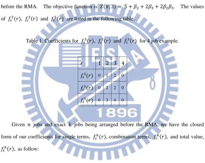
For illustration, we consider an example with 4 jobs and exact 3 jobs being arranged before the RMA. The objective function is 𝑍 𝜋, 3 = 5 + 𝛽 + 2𝛽 + 2𝛽 𝛽 . The values of , and are listed in the following table.

Table 1. Coefficients for , and for 4 job example.

r 1 2 3 4 0 1 2 0

0 2 2 0

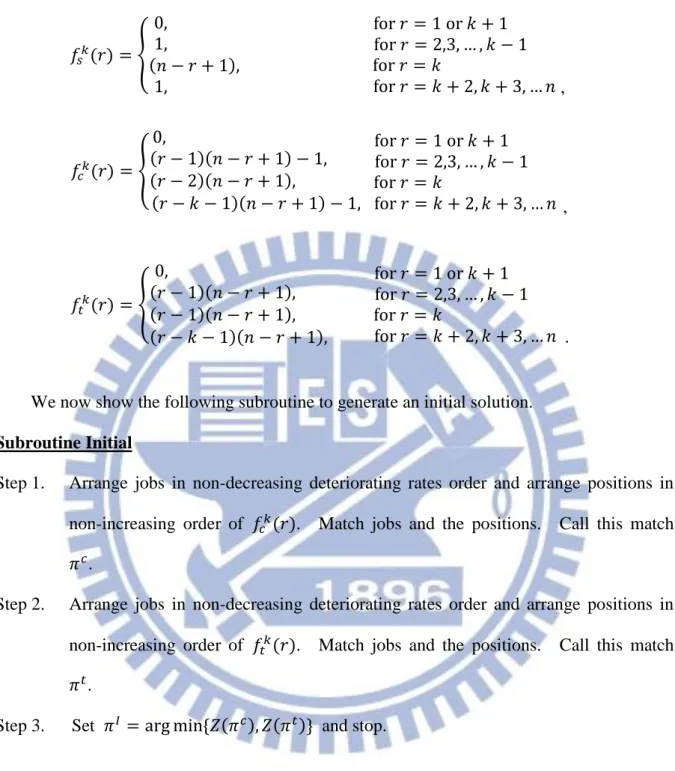
0 3 4 0

Given 𝑛 jobs and exact 𝑘 jobs being arranged before the RMA, we have the closed form of our coefficients for single terms, 𝑘 , combination terms, 𝑘 , and total value,

17

We now show the following subroutine to generate an initial solution. Subroutine Initial

Step 1. Arrange jobs in non-decreasing deteriorating rates order and arrange positions in non-increasing order of 𝑘 . Match jobs and the positions. Call this match 𝜋 .

Step 2. Arrange jobs in non-decreasing deteriorating rates order and arrange positions in non-increasing order of 𝑘 . Match jobs and the positions. Call this match 𝜋 .

Step 3. Set 𝜋 = r min {𝑍 𝜋 , 𝑍 𝜋 } and stop.

For illustration, we take a 10 job example and exact 5 jobs are arranged before RMA. Table 2. Deteriorating rates of a 10 job example.

𝑗 1 2 3 4 5 6 7 8 9 10 𝛼_𝑗 0.39 0.69 0.78 0.82 1.55 1.56 2.08 2.54 3.32 4.92 𝛽_𝑗 1.39 1.69 1.78 1.82 2.55 2.56 3.08 3.54 4.32 5.92 . 𝑓_𝑐𝑘 _{𝑟 =} 0, 𝑟 − 1 𝑛 − 𝑟 + 1 − 1, 𝑟 − 2 𝑛 − 𝑟 + 1 , 𝑟 − 𝑘 − 1 𝑛 − 𝑟 + 1 − 1, 𝑓_𝑠𝑘 _{𝑟 =} 0, 1, 𝑛 − 𝑟 + 1 , 1, for 𝑟 = 1 or 𝑘 + 1 for 𝑟 = 2,3, … , 𝑘 − 1 for 𝑟 = 𝑘 for 𝑟 = 𝑘 + 2, 𝑘 + 3, … 𝑛 𝑓𝑡𝑘 𝑟 = 0, 𝑟 − 1 𝑛 − 𝑟 + 1 , 𝑟 − 1 𝑛 − 𝑟 + 1 , 𝑟 − 𝑘 − 1 𝑛 − 𝑟 + 1 , for 𝑟 = 1 or 𝑘 + 1 for 𝑟 = 2,3, … , 𝑘 − 1 for 𝑟 = 𝑘 for 𝑟 = 𝑘 + 2, 𝑘 + 3, … 𝑛 for 𝑟 = 1 or 𝑘 + 1 for 𝑟 = 2,3, … , 𝑘 − 1 for 𝑟 = 𝑘 for 𝑟 = 𝑘 + 2, 𝑘 + 3, … 𝑛 , ,

18

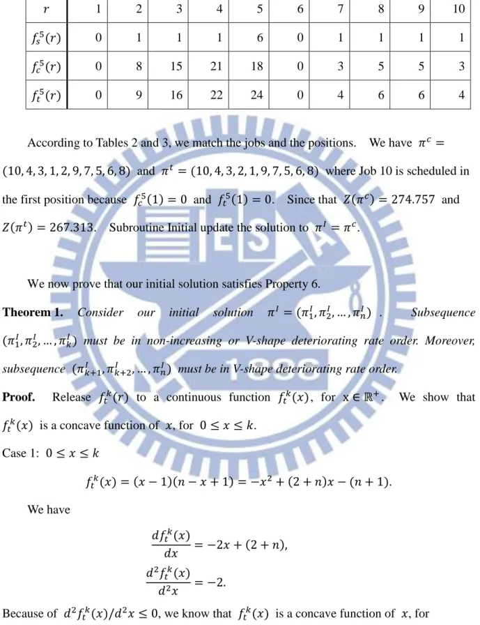
Table 3. Coefficients for , and for a 10 job example.

1 2 3 4 5 6 7 8 9 10

0 1 1 1 6 0 1 1 1 1

0 8 15 21 18 0 3 5 5 3

0 9 16 22 24 0 4 6 6 4

According to Tables 2 and 3, we match the jobs and the positions. We have 𝜋 = 10, 4, 3, 1, 2, 9, 7, 5, 6, 8 and 𝜋 = 10, 4, 3, 2, 1, 9, 7, 5, 6, 8 where Job 10 is scheduled in the first position because 1 = 0 and 1 = 0. Since that 𝑍 𝜋 = 274.757 and 𝑍 𝜋 = 267.313. Subroutine Initial update the solution to 𝜋 = 𝜋 .

We now prove that our initial solution satisfies Property 6.

Theorem 1. Consider our initial solution 𝜋 = 𝜋 , 𝜋 , … , 𝜋 . Subsequence 𝜋 , 𝜋 , … , 𝜋_𝑘 must be in non-increasing or V-shape deteriorating rate order. Moreover, subsequence 𝜋_𝑘+ , 𝜋_𝑘+ , … , 𝜋 must be in V-shape deteriorating rate order.

Proof. Release 𝑘 to a continuous function 𝑘 , for x ℝ+. We show that

𝑘 _{is a concave function of , for 0 ≤ ≤ 𝑘.}

Case 1: 0 ≤ ≤ 𝑘 𝑘 _{= − 1 𝑛 − + 1 = − + 2 + 𝑛 − 𝑛 + 1 .} We have 𝑑 𝑘 𝑑 = −2 + 2 + 𝑛 , 𝑑 𝑘 𝑑 = −2.

Because of 𝑑 𝑘 /𝑑 ≤ 0, we know that 𝑘 is a concave function of , for 0 ≤ ≤ 𝑘. The global optimum at ∗ _{= 𝑛 + 2 /2 > 0. Because} ∗ _{≥ 0,} 𝑘 _will

19

not be monotonic decreasing function.

Then, we show that 𝑘 is a concave function of for 𝑘 + 1 ≤ ≤ 𝑛. Case 2: 𝑘 + 1 ≤ ≤ 𝑛 𝑘 _{= − 𝑘 − 1 𝑛 − + 1 = − + 𝑛 + 𝑘 + 2 − 𝑘𝑛 + 𝑘 + 𝑛 + 1 .} We have 𝑑 𝑘 𝑑 = −2 + 𝑛 + 𝑘 + 2 , 𝑑 𝑘 𝑑 = −2.

Because of 𝑑 𝑘 /𝑑 ≤ 0, we know that 𝑘 is a concave function of , for 0 ≤ ≤ 𝑘.

Since that 𝑘 is a concave function for x ℝ+ and our initial solution is to assign the jobs with larger deteriorating rate to the position with the small coefficient. Our initial solution satisfies properties 6. ∎

After we have our initial solution, we show our Subroutine Improvement One. Subroutine Improvement One

Step 1. Input 𝜋 = 𝜋 , 𝜋 , … 𝜋 where 𝑝 = r m x𝑖= , ,…,𝑘{𝛽_𝜋𝑖} and

𝑞 = r m x𝑖=𝑘+ ,𝑘+ ,…, {𝛽_𝜋𝑖}. Swap 𝜋 and 𝜋𝑞. Call this new sequence 𝜋 .

Step 2.1 Arrange 𝜋 , 𝜋 , … , 𝜋_𝑘 in non-decreasing deteriorating rates order and arrange positions in non-increasing order of 𝑘 , for = 1,2, … , 𝑘. Match jobs and the positions and update match 𝜋 .

Step 2.2 Arrange 𝜋_𝑘+ , 𝜋_𝑘+ , … , 𝜋 in non-decreasing deteriorating rates order and arrange positions in non-increasing order of 𝑘 , for = 𝑘 + 1, 𝑘 + 2, … , 𝑛. Match jobs and the positions and update match 𝜋 .

20

To illustrate Subroutine Improvement One, we adopt the same example. With initial solution 𝜋 = 10, 4, 3, 1, 2, 9, 7, 5, 6, 8 , we swap Job 8 and Job 4 and get 𝜋 = 10, 8, 3, 2, 1, 9, 6, 4, 5, 7 . Since that 𝑍 𝜋 = 274.757 and 𝑍 𝜋 = 267.313 . Subroutine Improvement One update the initial solution to 𝜋 = 𝜋 .

To show our Subroutine Improvement Two, define:

Finally, we show our Subroutine Improvement Two. Subroutine Improvement Two

Step 1. Input 𝜋 . Set ℎ = 0 and 𝜋 = 𝜋 . Step 2. For 𝜋 ℎ , calculate 𝐶_𝑘 ℎ and _𝑘 ℎ .

Step 3. Arrange jobs in non-decreasing deteriorating rates order and arrange positions in non-increasing order of _𝑘 ℎ . Match jobs and the positions. Call this match 𝜋 ℎ+ _.

Step 4. If 𝑍(𝜋 ℎ ) > 𝑍(𝜋 ℎ+ ), then set ℎ = ℎ + 1 and go to step 2. Otherwise, set 𝜋𝑘 =𝜋 ℎ and stop.

To illustrate Subroutine Improvement Two, we adopt the same example. With solution 𝜋 _{= 𝜋 = 10, 8, 3, 2, 1, 9, 6, 4, 5, 7 , we calculate in Table 4 and rematch our}

jobs and the positions and get 𝜋 = 10, 6, 3, 2, 1, 9, 7, 4, 5, 8 . Since 𝑍(𝜋 ) =

𝑘 = 𝐶_𝑘 𝛽 _. 𝐶𝑘 𝑟 = 𝛽𝑣 _𝑠 𝑠=𝑖 𝑘 𝑣=𝑟 𝑟 𝑖= + 𝑛 − 𝑘 𝛽𝑠 𝑘 𝑠=𝑖 𝑟 𝑖= , 𝛽𝑠 , 𝑣 𝑠=𝑖 𝑛 𝑣=𝑟 𝑟 𝑖=𝑘+ for 𝑟 = 1,2, … , 𝑘 for 𝑟 = 𝑘 + 1, 𝑘 + 2, … , 𝑛 ,

21

267.3313 and 𝑍(𝜋 _{) = 259.233, we calculate in Table 4 and rematch again}

and get 𝜋 = 10, 6, 3, 2, 1, 9, 7, 4, 5, 8 . Since 𝑍(𝜋 ) = 𝑍(𝜋 ) , Subroutine Improvement Two update our solution to 𝜋𝑘=𝜋 1 .

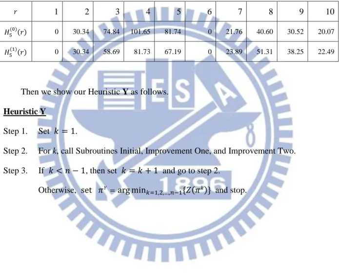
Table 4. and for Subroutine Improvement Two

1 2 3 4 5 6 7 8 9 10

0 30.34 74.84 101.65 81.74 0 21.76 40.60 30.52 20.07

0 30.34 58.69 81.73 67.19 0 23.89 51.31 38.25 22.49

Then we show our Heuristic Y as follows. Heuristic Y

Step 1. Set 𝑘 = 1.

Step 2. For k, call Subroutines Initial, Improvement One, and Improvement Two. Step 3. If 𝑘 < 𝑛 − 1, then set 𝑘 = 𝑘 + 1 and go to step 2.

22

Chapter 5. Experiment design and numerical study

We design different scenarios with different parameter. Under each scenario, we randomly generate 30 examples to verify the efficiency of the proposed heuristic.

5.1 Generating of experiment data

Without loss of generality, we set the value of the duration of RMA 𝑡 = 0. The scenarios are designed as follows: (i) The number of jobs n is from 3 to 12; and (ii) The deteriorating rates α is following uniform distributions of U 0,1 , U 0,3 , U 0,5 , U 0,10 , U 0,20 , U 0,30 , U 0,40 , U 10,40 , U 20,40 and U 30,40 . Therefore, we consider 100 scenarios in our numerical studies. For each scenario, we generate 30 examples. Totally, there are 3000 examples in our numerical study.

5.2 Experiment results

We determine the near optimal sequence of jobs and RMA and its flow time 𝑍𝑌 by the proposed heuristic stated in Chapter 4 for each example. We also use exhaustive search to find the exactly optimal sequence of jobs and RMA and its flow time 𝑍𝑘∗ . Then we mean the relative errors and the computational times of 30 examples in each scenario. The relative error is defined as

R l iv rror % = 𝑍𝑌− 𝑍∗

𝑍∗ × 100%.

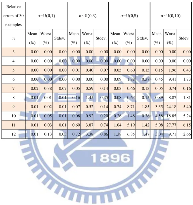
Tables 5 and 6 show the mean relative error, the worst relative error and the standard deviation of each scenario.

23

Table 5. Relative errors for α~U 0,1 ,α~U 0,3 ,α~U 0,5 and α~U 0,10

Relative errors of 30

examples

α~U 0,1 α~U 0,3 α~U 0,5 α~U 0,10

𝑛 Mean (%) Worst (%) Stdev. Mean (%) Worst (%) Stdev. Mean (%) Worst (%) Stdev. Mean (%) Worst (%) Stdev. 3 0.00 0.00 0.00 0.00 0.00 0.00 0.00 0.00 0.00 0.00 0.00 0.00 4 0.00 0.00 0.00 0.00 0.00 0.00 0.00 0.00 0.00 0.00 0.00 0.00 5 0.00 0.00 0.00 0.01 0.40 0.07 0.05 0.60 0.15 0.15 1.96 0.43 6 0.00 0.00 0.00 0.00 0.00 0.00 0.09 1.88 0.37 0.45 9.41 1.73 7 0.02 0.38 0.07 0.05 0.59 0.14 0.03 0.66 0.13 0.05 0.74 0.16 8 0.01 0.01 0.01 0.16 1.45 0.35 0.08 0.63 0.15 0.89 8.87 1.81 9 0.01 0.02 0.01 0.07 0.52 0.14 0.74 8.71 1.85 3.35 24.18 5.40 10 0.01 0.05 0.01 0.08 0.92 0.20 0.26 1.48 0.36 4.58 18.85 5.24 11 0.01 0.03 0.01 0.60 3.87 0.74 1.04 5.19 1.42 5.08 27.77 6.15 12 0.01 0.13 0.03 0.72 3.38 0.86 1.38 6.85 1.47 3.04 9.71 2.66

24

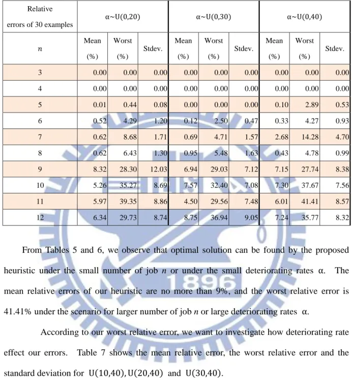
Table 6. Relative errors for α~U 0,20 ,α~U 0,30 and α~U 0,40

From Tables 5 and 6, we observe that optimal solution can be found by the proposed heuristic under the small number of job n or under the small deteriorating rates α. The mean relative errors of our heuristic are no more than 9%, and the worst relative error is 41.41% under the scenario for larger number of job n or large deteriorating rates α.

According to our worst relative error, we want to investigate how deteriorating rate effect our errors. Table 7 shows the mean relative error, the worst relative error and the standard deviation for U 10,40 , U 20,40 and U 30,40 .

Relative errors of 30 examples

α~U 0,20 α~U 0,30 α~U 0,40

𝑛 Mean (%) Worst (%) Stdev. Mean (%) Worst (%) Stdev. Mean (%) Worst (%) Stdev. 3 0.00 0.00 0.00 0.00 0.00 0.00 0.00 0.00 0.00 4 0.00 0.00 0.00 0.00 0.00 0.00 0.00 0.00 0.00 5 0.01 0.44 0.08 0.00 0.00 0.00 0.10 2.89 0.53 6 0.52 4.29 1.20 0.12 2.50 0.47 0.33 4.27 0.93 7 0.62 8.68 1.71 0.69 4.71 1.57 2.68 14.28 4.70 8 0.62 6.43 1.30 0.95 5.48 1.63 0.43 4.78 0.99 9 8.32 28.30 12.03 6.94 29.03 7.12 7.15 27.74 8.38 10 5.26 35.27 8.69 7.57 32.40 7.08 7.30 37.67 7.56 11 5.97 39.35 8.86 4.50 29.56 7.48 6.01 41.41 8.57 12 6.34 29.73 8.74 8.75 36.94 9.05 7.24 35.77 8.32

25

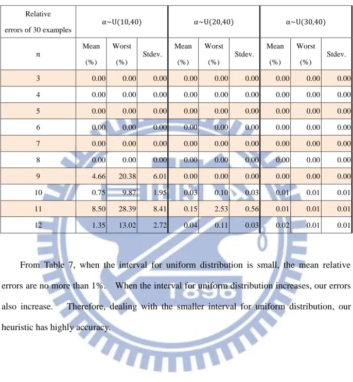
Table 7. Relative errors for α~U 10,40 ,α~U 20,40 and α~U 30,40

From Table 7, when the interval for uniform distribution is small, the mean relative errors are no more than 1%. When the interval for uniform distribution increases, our errors also increase. Therefore, dealing with the smaller interval for uniform distribution, our heuristic has highly accuracy.

Relative errors of 30 examples

α~U 10,40 α~U 20,40 α~U 30,40

𝑛 Mean (%) Worst (%) Stdev. Mean (%) Worst (%) Stdev. Mean (%) Worst (%) Stdev. 3 0.00 0.00 0.00 0.00 0.00 0.00 0.00 0.00 0.00 4 0.00 0.00 0.00 0.00 0.00 0.00 0.00 0.00 0.00 5 0.00 0.00 0.00 0.00 0.00 0.00 0.00 0.00 0.00 6 0.00 0.00 0.00 0.00 0.00 0.00 0.00 0.00 0.00 7 0.00 0.00 0.00 0.00 0.00 0.00 0.00 0.00 0.00 8 0.00 0.00 0.00 0.00 0.00 0.00 0.00 0.00 0.00 9 4.66 20.38 6.01 0.00 0.00 0.00 0.00 0.00 0.00 10 0.75 9.87 1.95 0.03 0.10 0.03 0.01 0.01 0.01 11 8.50 28.39 8.41 0.15 2.53 0.56 0.01 0.01 0.01 12 1.35 13.02 2.72 0.04 0.11 0.03 0.02 0.01 0.01

26

We show the mean computational times in Table 8 and graph the results in Figure 3.

Table 8. Computational times

Mean Computational times (sec.) Heuristic Y Exhaustive search 𝑛 = 3 0.0314 0.0018 𝑛 = 4 0.0504 0.0024 𝑛 = 5 0.0738 0.0026 𝑛 = 6 0.0966 0.0030 𝑛 = 7 0.1260 0.0040 𝑛 = 8 0.1620 0.0166 𝑛 = 9 0.2104 0.1478 𝑛 = 10 0.2540 1.8026 𝑛 = 11 0.3102 23.6875 𝑛 = 12 0.3958 339.6359

Figure 3. Computational times

0 50 100 150 200 250 300 350 3 4 5 6 7 8 9 10 11 12 Time (sec.) Number of jobs Heuristic Y Exhaustive search

27

From Table 8 and Figure 3, when the number of jobs is less than ten, the computational times of exhaustive search are less than those of our proposed heuristic. When the number of jobs increases, the computational times of exhaustive search increase significantly. But the computational times of our proposed heuristic under the large number of job size is increase slightly.

Chapter 6. Conclusions and future researches

In this paper, we consider a scheduling problem of deteriorating jobs and single RMA on a single machine. Our objective is to minimize the flow time and the main purpose is to determine the sequence of jobs and RMA. We first examine the complexity of our problem. Then we purpose some optimality properties. Besides, we also find that the coefficients of the objective function are the key factor to determine the value of flow time. Based on those properties, we propose a heuristic to solve the problem.

In order to validate the performance of our heuristic, we randomly generate examples among some scenarios and do the numerical studies. Then, with the proposed heuristic, we find that the mean relative errors of our heuristic in all examples are no more than 9%. The computational times with the proposed heuristic are not significantly increasing in the examples of large job size n.

In the future, we would like to improve our mean relative errors first. We could also study problem for different scenario. For example, we extend our problem to multiple RMAs with multiple machines. We could also consider different deteriorating function such as step function and quadratic function.

28

Reference

Bachman, A., Janiak, A., and Kovalyov, M.Y., 2002. Minimizing the total weighted completion time of deteriorating jobs. Information Processing Letters 81, 81-84 Browne, S., and Yechiali, U., 1990. Scheduling deteriorating jobs on a single

process. Operations Research 38, 495-498.

Gupta, J.N.D., and Gupta, S.K., 1988. Single facility scheduling with nonlinear processing times. Computers & Industry Engineering 14, 387-393.

Kubale, M., and Ocetkiewicz, K.M., 2009. A new optimal algorithm for a time-dependent scheduling problem. Control and Cybernetics 38, 713-721. Lee, C.Y., and Leon V.J., 2001. Machine scheduling with rate-modifying activity.

European Journal of Operational Research 128, 119-128.

Lee, C.Y., and Lin, C.S., 2001. Single-machine scheduling with maintenance and repair rate modifying activities. European Journal of Operational Research 135, 493-513.

Lodree, E.J. and Geiger, C.D., 2010. A note on the optimal sequence position for a rate-modifying activity under simple linear deterioration, European Journal of Operational Research 201(2), 644-648

Mosheiov, G., 1991. V-shaped policies for scheduling deteriorating jobs. Operations Research 39, 979-991.

Mosheiov, G., 1994. Scheduling jobs under linear deterioration. Computers & Operations Research 21, 653-659.

Mosheiov, G., 1995. Scheduling jobs with step-deterioration: minimizing makespan on single and multi-machine. Computers & Industry Engineering 28, 869-879. Mosheiov, G., 2002. Complexity analysis of job-shop scheduling with deteriorating

29

Mosheiov, G., 2005. A note on scheduling deteriorating jobs. Mathematical and Computer Modeling 41, 883-886.

Ozturkoglu, Y. and Bulfin, R.L., 2010. A unique integer mathematical model for scheduling deteriorating jobs with rate-modifying activities on a single machine. The International Journal of Advanced Manufacturing Technology, DOI:10.1007/s00170-011-3303-9

Zhao, C.L., Tang, H.Y., and Cheng, C.D., 2009. Two-parallel machines scheduling with rate-modifying activities to minimize total completion time. European Journal of Operational Research 198, 354-357.