國
立
交
通
大
學
網路工程研究所
碩
士
論
文
無線隨意網路在具不可靠節點與
連線環境中之網路連通性
Connectivity of the Wireless Ad Hoc Networks
with Unreliable Nodes and Links
研 究 生:林國維
指導教授:易志偉
無線隨意網路在具不可靠節點與連線環境中之網路連通性
Connectivity of the Wireless Ad Hoc Networks
with Unreliable Nodes and Links
研 究 生:林國維 Student:Kuo-Wei Lin
指導教授:易志偉 Advisor:Chih-Wei Yi
國 立 交 通 大 學
網 路 工 程 研 究 所
碩 士 論 文
A ThesisSubmitted to Institute of Network Engineering College of Computer Science
National Chiao Tung University in partial Fulfillment of the Requirements
for the Degree of Master
in
Computer Science July 2007
Hsinchu, Taiwan, Republic of China
Connectivity of the Wireless Ad Hoc
Networks with Unreliable Nodes and Links
Student: Kuo-Wei Lin
Advisor: Dr. Chih-Wei Yi
Institute of Network Engineering
National Chiao Tung University
Abstract
In randomly-deployed wireless ad hoc networks with reliable nodes and links, vanish-ment of isolated nodes asymptotically implies connectivity of networks. However, in a realistic system, nodes may become inactive, and links may become down. The inactive nodes and down links cannot take part in routing/relaying and thus may affect the con-nectivity. In this paper, we study the connectivity of a wireless ad hoc network that is composed of unreliable nodes and links by investigating the distribution of the number of isolated nodes in the network. We assume that the wireless ad hoc network consists of n nodes which are distributed independently and uniformly in an unit-area disk or square. Nodes are active independently with probability 0 < p1 ≤ 1, and links are up
independently with probability 0 < p2 ≤ 1. A node is said to be isolated if it doesn’t
have an up link to active nodes. We show that if all nodes have a maximum transmis-sion radius rn=
q
ln n+ξ
πp1p2n for some constant ξ, then the total number of isolated nodes is
asymptotically Poisson with mean p1e−ξ. In addition, the work can be extended for secure
wireless networks which adopt m-composite key predistribution schemes or multiple-space key predistribution scheme in which a node is said to be isolated if it doesn’t have a secure link to its neighbor nodes. Let p denote the probability of the event that two neighbor nodes have a secure link. We show that if all nodes have a maximum transmission radius
rn =
q
ln n+ξ
πpn for some constant ξ, then the total number of isolated nodes is
asymptoti-cally Poisson with mean e−ξ. We also give extensive simulations. The convergence of the
asymptotic critical transmission radius was verified by simulations. In our simulations, various network scenarios were considered, and the average and cumulative distribution function of critical transmission radii were investigated.
Keywords
Connectivity, isolated nodes, asymptotic distribution, random geometric graphs, ran-dom key predistribution.
Contents
List of Figures vii List of Tables viii
1 Introduction 1
1.1 What is the Wireless Ad Hoc Network . . . 1 1.2 Motivation and Model . . . 2 1.3 Related Works . . . 3
2 Preliminaries 5
2.1 Geometry of Disks . . . 6 2.2 Limits of integrals . . . 11
3 Main Results 20
3.1 Wireless Ad Hoc Newtorks with Bernoulli Model . . . 20 3.2 Key Predistribution Scheme . . . 23 4 Asymptotic Distribution of The Number of Isolated Nodes 26 4.1 Networks with Bernoulli Nodes and Links . . . 27
4.2 Secure Wireless Networks . . . 31
5 Simulations and Conclusions 34 5.1 Simulation Setup and Notations . . . 34
5.2 Native Models . . . 36
5.3 Networks with Bernoulli Nodes . . . 38
5.4 Networks with Bernoulli Nodes and Links . . . 44
5.5 Secure Wireless Networks . . . 52
5.6 Conclusions . . . 54
List of Figures
2.1 The partitions of the unit-area disk Ω. . . 6
2.2 The half-disk and the triangle. . . 7
2.3 The area of two intersecting disks. . . 8
5.1 The r-disk graph over an unit-area disk. . . 36
5.2 The c.d.f. of CTR’s of r-disk graphs over an unit-area disk. . . 37
5.3 The r-disk graph over an unit-area disk with unreliable nodes. . . 38
5.4 The c.d.f. of CTR’s over an unit-area disk with unreliable nodes. . . 39
5.5 The c.d.f. of CTR’s over an unit-area square with unreliable nodes. . . 42
5.6 The r-disk graph with waking/sleeping nodes and listening links. . . 43
5.7 The c.d.f. of CTR’s with waking/sleeping nodes and listening links. . . 45
5.8 The r-disk graph with unreliable nodes and links. . . 47
5.9 The c.d.f. of CTR’s with unreliable nodes and links. . . 48
5.10 The c.d.f. of CTR’s with waking/sleeping nodes and unreliable links. . . . 51
5.11 The secure networks with K = 40, k = 10, and m = 2. . . 52
List of Tables
5.1 The average CTR’s corresponding to Figure 5.2. . . 37
5.2 The average CTR’s corresponding to Figure 5.4. . . 40
5.3 The average CTR’s corresponding to Figure 5.5. . . 41
5.4 The average CTR’s corresponding to Figure 5.7. . . 46
5.5 The average CTR’s corresponding to Figure 5.8. . . 49
5.6 The average CTR’s corresponding to Figure 5.10. . . 50
Chapter 1
Introduction
1.1
What is the Wireless Ad Hoc Network
A wireless ad hoc network is composed of a collection of wireless devices distributed over a geograhic region. Instead of wired lines, wireless devices transmit/receive data via omnidirectional antennas. A communacation session is established either through a single-hop radio transmission if the communication parties are close enough, or through relaying by intermediate devices otherwise. Routing is required to be done autonomously by the devices for multi-hop transmission. Due to no need for a fixed infrastructure, wireless ad hoc networks can be flexibly deployed at low cost for various missions. In many applications, wireless devices are deployed in a large volume. The sheer large number of devices deployed coupled with the potential harsh environment often eliminates the possibility of strategic device placement. Consequently, random deployment is often the only viable option.
pro-posed in the last few years. In 2003, the IEEE 802.15.4 standard [1] was propro-posed as a MAC and PHY layer standard for low-rate wireless personal area ad hoc networks, and ZigBee specifications [2] were ratified in 2004 as one of the leading standards for wireless ad hoc and sensor networks. J. Zhu and S. Roy (2005) [3] proposed a mesh architec-ture based on two-radio 802.11 access points (AP’s). The IEEE 802.16 standard [4] also known as ”WiMAX” was approved in 2004, and the MAC layer supports a primarily point-to-multipoint architecture with an optional mesh topology.
1.2
Motivation and Model
The connectivity of wireless ad hoc networks is an essential problem. If a network is not connected, it seperates into several disconnected components. There are no commu-nication links between components. So devices in one component can not communicate with devices in other components. Intuitively, there is a tradeoff between the network connectivity and the transmission power of the devices. The larger the transmission power is, the more likely the network is connected. But larger transmission power costs more energy and causes serious interference. In this study, we would like to figure out a balance between network connectivity and transmission power.
To model a randomly deployed wireless ad hoc network, it is natural to represent the ad hoc devices by a finite random point process over the deployment region [5] [6] [7] [8] [9]. In addition, due to the short transmission range of radio links, two wireless devices can build a communication link only if they are within each other’s transmission range. Assume all devices have the same transmission radius r, then the induced network
topology is a r-disk graph in which two nodes are joined by an edge if and only if their distance is at most r. This is a variant of the model proposed by Gilbert (1961) [10] and referred as a random geometric graph.
1.3
Related Works
A node is said to be isolated if it does not have any 1-hop neighbors. The vanishment of isolated nodes in an ad hoc network is a prerequisite of network connectivity. The connectivity of random geometric graphs has been studied by Dette and Henze (1989) [11], Penrose (1997) [12], and others [5] [6] [13] [14]. For an uniform n-point process over an unit-area square, Dette and Henze (1989) [11] showed that for any constant ξ, the µq
ln n+ξ
πn
-disk graph has no isolated nodes with probability exp¡−e−ξ¢ asymptotically.
Later, Penrose (1997) [12] established that if a random geometric graph induced by an uniform point process or Poisson point process has no isolated nodes, then it is almost surely connected.
However, in a realistic system, nodes may become inactive due to, for example, inter-nal breakdown or being in the listening state, and links may become down due to, for example, harsh environment or barriers between nodes. The inactive nodes and down links cannot take part in routing/relaying and thus may affect the connectivity. To model the unreliability of nodes, Wan and Yi et al [6] [14] assume that every nodes independently break down with the same probability p. They showed that if the maximum transmis-sion radius of every nodes is
q
ln n+ξ
πpn for some constant ξ, the network is connected with
Based on the work in [6], we study a more general case of the connectivity of a wireless network with both unreliable nodes and links. We assume nodes are active independently with the same probability p1 and links are up independently with the same probability
p2. We show that if all nodes have a maximum transmission radius rn =
q
ln n+ξ
πp1p2n for
some constant ξ, then the total number of isolated nodes is asymptotically Poisson with mean e−ξ and the total number of isolated active nodes is also asymptotically Poisson
with mean p1e−ξ. In addition, the work can be extended for secure wireless networks with
m-composite key predistribution schemes [19] [20] [21] [23]. In many applications, the
wireless sensor networks are composed of low cost devices. Traditional security schemes and key management algorithms, such as Diffie-Hellman key agreement [17] and RSA signatures [18], are too complex and not feasible for such systems. The m-composite key predistribution schemes are proposed to offer security for randomly-deployed wireless sensor networks, and are more adaptive to wireless sensor networks. We assume every links have probability p to be secure independently, and show that if all nodes have a maximum transmission radius rn =
q
ln n+ξ
πpn for some constant ξ, then the total number
of isolated nodes is asymptotically Poisson with mean e−ξ.
The remaining of this paper is organized as follows. In chapter 2, we present several useful geometric results and integrals. In chapter 3, the main results of the study are given. The distribution of the number of isolated nodes is derived in chapter 4. In chapter 5, we give both simulation results and the conclusions.
Chapter 2
Preliminaries
In preparation for our main study, we adopt notations and terminologies used in [6]. For completeness, we give their definitions here. Most lemmas in this chapter can also be found corresponding ones in [6].
In what follows, all integrals considered will be Lebesgue integrals. For any set S and positive integer k, the k-fold Cartesian product of S is denoted by Sk. kxk is the Euclidean
norm of a point x ∈ R2, and |x| is the shorthand for 2-dimensional Lebesgue measure (or
area) of a measure set A ⊂ R2. The topological boundary of a set A ⊂ R2 is denoted by
∂A. The disk of radius r centered at x is denoted by B (x, r). The special unit-area disk
or square centered at the origin o is denoted by Ω. The symbols o and ∼ always refer to the limit n → ∞. To avoid trivialities, we tacitly assume n to be sufficiently large if necessary. For simplicity of notation, the dependence of sets and random variables on n will be frequently suppressed.
Let r be the transmission radius of the nodes. For any finite set of nodes {x1, ..., xk}
an edge between two nodes if and only if their Euclidean distance is at most r. For any positive integers k and m with 1 ≤ m ≤ k, let Ckm denote the set of (x1, ..., xk) ∈ Ωk
satisfying that G2r(x1, ..., xk) has exactly m connected components.
2.1
Geometry of Disks
00000000000 00000000000 00000000000 00000000000 00000000000 00000000000 00000000000 00000000000 00000000000 00000000000 00000000000 00000000000 00000000000 00000000000 00000000000 00000000000 00000000000 00000000000 00000000000 00000000000 00000000000 00000000000 11111111111 11111111111 11111111111 11111111111 11111111111 11111111111 11111111111 11111111111 11111111111 11111111111 11111111111 11111111111 11111111111 11111111111 11111111111 11111111111 11111111111 11111111111 11111111111 11111111111 11111111111 11111111111 π 1 Ω(2) r Ω(0) Ω(1) r oFigure 2.1: The partitions of the unit-area disk Ω.
We partition the disk Ω into three regions Ω(0), Ω(1), Ω(2) centered at the origin o. As shown in Figure 2.1, Ω(0) is the disk of radius 1/√π − r; Ω(1) is the annulus of radii
1/√π − r and p1/π − r2; and Ω(2) is the annulus of radiip1/π − r2 and 1/√π. Then
the areas of the three partitions are
|Ω(0)| = (1/√π − r)2π = (1 −√πr)2,
|Ω(1)| = (p1/π − r2)2π − (1 −√πr)2 = 2πr(1/√π − r),
|Ω(2)| = πr2.
For any set S ⊆ Ω and r > 0, the r-neighborhood of S is the set Sx∈SB (x, r) ∩ Ω.
000000 000000 000000 000000 000000 000000 000000 000000 000000 000000 000000 000000 000000 000000 000000 000000 000000 000000 000000 000000 000000 111111 111111 111111 111111 111111 111111 111111 111111 111111 111111 111111 111111 111111 111111 111111 111111 111111 111111 111111 111111 111111
000
000
000
000
000
000
000
000
000
000
000
111
111
111
111
111
111
111
111
111
111
111
o x y b aFigure 2.2: The half-disk and the triangle.
abusing the notation, to denote the r-neighborhood of S itself. Ovbiously, for any x ∈ Ω,
vr(x) ≥ πr2/3. If x ∈ Ω(0), vr(x) = πr2. If x ∈ Ω(1), Lemma 1 gives a tighter lower
bound on vr(x).
Lemma 1 For any x ∈ Ω(1),
vr(x) ≥ πr2 2 + µ 1 √ π − kxk ¶ r.
Proof. Intuitively, the transmission radius of Ω = kyk = 1/√π. Let y be the point
in ∂Ω such that ky − xk = √1
π − kxk, and ab be the diameter of B (x, r) perpendicular to
xy (see Figure 2.2). Then vr(x) contains a half-disk of B (x, r) to the side of ab opposite
to y, and the triangle aby. Since the area of the triangle aby is exactly ³ 1 √ π − kxk ´ r, the lemma follows.
Lemma 2 Assume that
r ≤ 1/ √ π 12/π + π/12 ≈ 0.245/ √ π.
Figure 2.3: The area of two intersecting disks.
Let x1, ..., xk be a sequence of k ≥ 2 nodes in Ω such that x1 has the largest norm, and
kxi− xjk ≤ 2r if and only if |i − j| ≤ 1. then
vr(x1, ..., xk) ≥ vr(x1) + π 12r k−1 X i=1 kxi+1− xik .
Proof. We prove the lemma by induction on k. When k = 2, let t = kx2− x1k and
f (t) = |B (x2, r) /B (x1, r)|. First, we show that f (t) ≥ (π/2) rt. As shown in Figure
2.3(a), let y1y2 be the common chord of ∂B (x1, r) and ∂B (x2, r), and z1z2 be another
chord of ∂B (x2, r) that is parallel to y1y2 and has the same length as y1y2. Then f (t) is
also equal to the area of the portion of B (x2, r) between the two chords y1y2 and z1z2.
Thus, f0(t) = ky
1y2k, which is decreasing over [0, 2r]. Therefore, f (t) is concave over
[0, 2r]. Since f (0) = 0 and f (2r) = πr2, we have f (t) ≥ (π/2) rt.
Now we are ready to prove the lemma for k = 2. If x1 ∈ Ω (0), then vr(x1, x2)−vr(x1)
is exactly f (t), and thus the lemma follows immediately from f (t) ≥ (π/2) rt. So we assume that x1 ∈ Ω (0). Note that for the same distance t, v/ r(x1, x2) − vr(x1) achieves
its minimum when both x1 and x2 are in ∂Ω. It is sufficient to prove the lemma for
x1, x2 ∈ ∂Ω. As shown in Figure 2.3(b), let y1y2 and z1z2 be the two chords of ∂B (x2, r)
as above with y2 ∈ Ω, and ` be the line through the two intersection points between ∂Ω
and ∂ (B (x1, r) ∪ B (x2, r)). A1 denotes the portion of B (x2, r) \B (x1, r) which lies in
the same side of ` as y2; A2 denotes the portion of B (x2, r) which is surrounded by y1y2,
z1z2, `, and the short arc between y2 and z2; and A3 denotes the rectanle surrounded by
y1y2, z1z2, `, and the line through x1 and x2. Intuitively, |A1| = |A2|. Then
vr(x1, x2) − vr(x1) ≥ |A1| = |A2| = f (t) /2 − |A3| .
An upper bound on |A3| can be obtained as follows. Let a be the intersection point
between y1y2 and `, b be the intersection point between y1y2 and ∂Ω, and c be the
intersection point between ` and ∂Ω. See Figure 2.3(c). Then kack ≤ 2r, and
koak = q kock2− kack ≥ r 1 π − (2r) 2. Hence,
kabk = kobk − koak ≤ 1 π − r 1 π − (2r) 2 = 4r 2 1 π + q 1 π − (2r) 2
Note that one side of A3 is exactly t and the other side is at most kabk. Thus
|A3| ≤ 4r2 1 π + q 1 π − (2r) 2
As f (t) ≥ (π/2) rt, we have vr(x1, x2) − vr(x1) ≥ f (t) /2 − |A3| = π 4 − 4r 1 π + q 1 π − (2r) 2 rt It is straightforward to verify that if
r ≤ 1/ √ π 12/π + π/12 ≈ 0.245/ √ π, then π 4 − 4r 1 π + q 1 π − (2r) 2 ≥ π 12 and thereby the lemma for k = 2 follows.
In the next, we assume the lemma is true for at most k − 1 nodes. We shall show that the lemma is true for k nodes. If k = 3, then
vr(x1, x2, x3) ≥ vr(x1) + vr(x3) ≥ vr(x1) + πr2 3 = vr(x1) + π 12r · 2 · 2r ≥ vr(x1) + π 12 2 X i=1 kxi+1− xik .
If k > 3, then by the induction hypothesis
vr(x1, ..., xk) ≥ vr(x1, ..., xk−2) + vr(xk) ≥ vr(x1) + π 12 k−3 X i=1 kxi+1− xik + π 12r · 4r ≥ vr(x1) + π 12 k−1 X i=1 kxi+1− xik
Corollary 3 Assume that r ≤ 1/ √ π 12/π + π/12 ≈ 0.245/ √ π.
Then for any (x1, ..., xk) ∈ Ck1 with x1 being the one of the largest norm among x1, ..., xk,
vr(x1, ..., xk) ≥ vr(x1) +
π
12r max2≤i≤kkxi− x1k .
Proof. Without loss of generality, we assume that kxk− x1k achieves
max2≤i≤kkxi− x1k. Let P be a path between x1 and xk with minimum hop counts
in G2r(x1, x2, ..., xk) and t be the total length of P . Then every pair of nodes in P that
does not establish a link (not adjacent) are seperated by a distance of more than 2r. Thus by applying Lemma 2 to the nodes in P , we obtain
vr({xi | xi ∈ P }) ≥ vr(x1) + π
12rt. Since vr(x1, ..., xk) ≥ vr({xi | xi ∈ P }) and t ≥ kxk− x1k, we have
vr(x1, ..., xk) ≥ vr({xi | xi ∈ P }) ≥ vr(x1) + π 12r kxk− x1k ≥ vr(x1) + π 12r max2≤i≤kkxi− x1k ,
and the corollary follows.
2.2
Limits of integrals
In the remaining of this chapter, we give the limits of several integrals which is useful for chapter 4. Similar lemmas can be found in [6].
Lemma 4 For any z ∈£0,1 2
¤
,
e−z−z2 ≤ 1 − z ≤ e−z.
Proof. For any z ≥ 0, 1 − z ≤ e−z ≤ 1 − z + z2
2 . If z ∈ £0,1 2 ¤ , then ez−z2 ≤ µ 1 − z + z 2 2 ¶ µ 1 − z2+z4 2 ¶ = 1 − z − z2 µ 1 2− z ¶ − 1 4z 5(2 − z) ≤ 1 − z,
and the lemma follows.
Lemma 5 If limn→∞p ln n = ∞ and r =
q
ln n+ξ
πpn for some constant ξ, then
n Z Ω e−npvr(x)dx ∼ e−ξ, n Z Ω (1 − pvr(x))n−1dx ∼ e−ξ. Proof. By Lemma 4, e−pvr(x)−(pvr(x))2 ≤ 1 − pv r(x) ≤ e−pvr(x). Then e−npvr(x)−n(pvr(x))2 ≤ (1 − pv r(x))n≤ e−npvr(x). Therefore, e−npvr(x)−npvr(x)2 = e−npvr(x)· e−npvr(x)2 = e−npvr(x)· e−c ln2 nn = e−npvr(x).
Note that npvr(x) = c ln n, 13 ≤ c ≤ 1. Thus, n (pvr(x))2 = (npvr(x))2 n = c2ln 2n n ∼ 0.
By the squeeze theorem, we have
n Z Ω (1 − pvr(x))n−1dx ∼ n Z Ω e−npvr(x)dx,
and the second equality would follow from the first one. We only have to give the proof of the first asymptotic equiality. First we calculate the integration over Ω (0).
n Z Ω(0) e−npvr(x)dx ≤ ne−npπr2|Ω (0)| ∼ ne−npπr2 = e−ξ.
Next, we calculate the integration over Ω (2) .
n Z Ω(2) e−npvr(x)dx ≤ ne−13npπr2|Ω (2)| = nπr2e−1 3npπr2 = o (1) .
Now we calculate the integration over Ω (1). By Lemma 1, n Z Ω(1) e−npvr(x)dx ≤ ne−npπr22 n Z Ω(1) e−npr “ 1 √ π−kxk ” dx = 2πne−npπr22 Z √1 π−r2 1 √ π−r pe−npr “ 1 √ π−ρ ” dρ ≤ 2πne−npπr22 Z √1 π 1 √ π−r pe−npr “ 1 √ π−ρ ” dρ ≤ 2√πne−npπr22 Z √1 π 1 √ π−r e−npr “ 1 √ π−ρ ” dρ = 2√πne−npπr22 Z r 0 e−nprtdt ≤ 2 √ π p 1 re −npπr22 = O (1) (ln n)−12 = o (1) . Therefore, n Z Ω e−npvr(x)dx ∼ e−ξ.
Lemma 6 If limn→∞p ln n = ∞ and r =
q
ln n+ξ
πpn for some constant ξ, then for any fixed
integer k ≥ 2, nk Z Ck1 e−npvr(x1,x2,··· ,xk) k Y i=1 dxi = o (1) , nk Z Ck1 (1 − pvr(x1, x2, · · · , xk))n−k k Y i=1 dxi = o (1) . Proof. Since (1 − pvr(x1, x2, · · · , xk))n−k ≤ e −npvr(x1,x2,··· ,xk) (1 − pkπr2)k ,
the second equality would follow from the first one. Hence, we only have to prove the first one. Let S denote the set of (x1, x2, ..., xk) ∈ Ck1 satisfying that x1 is the one with largest
norm among x1, ..., xk and x2 is the one with longest distance from x1 among x2, ..., xk.
Then nk Z Ck1 e−npvr(x1,x2,··· ,xk) k Y i=1 dxi ≤ k (k − 1) nk Z S e−npvr(x1,x2,··· ,xk) k Y i=1 dxi. It suffices to prove nk Z Ck1 e−npvr(x1,x2,··· ,xk) k Y i=1 dxi = o (1) .
Note that for any (x1, x2, ..., xk) ∈ S,
vr(x1) + cr kx2− x1k ≤ vr(x1, x2, ..., xk)
≤ kπr2
for some constant c, and
xi ∈ B (x1, kx2− x1k) , 3 ≤ i ≤ k;
Thus, nk Z S e−npvr(x1,x2,··· ,xk) k Y i=1 dxi ≤ nk Z S e−np(vr(x1)+crkx2−x1k) k Y i=1 dxi ≤ nk Z Ω e−npvr(x1)dx 1 Z B(x1,2(k−1)r) e−npcrkx2−x1kdx 2 k Y i=3 Z B(x1,kx2−x1k) dxi = nk Z Ω e−npvr(x1)dx 1 Z B(x1,2(k−1)r) e−npcrkx2−x1k¡π kx 2 − x1k2 ¢k−2 dx2 = 2πk−1 µ nk Z Ω e−npvr(x1)dx 1 ¶ Ã nk−1 Z 2(k−1)r 0 e−npcrρρ2k−3dρ ! < 2πk−1 µ nk Z Ω e−npvr(x1)dx 1 ¶ µ nk−1 Z ∞ 0 e−npcrρρ2k−3dρ ¶ = (2k − 3)!2π k−1nk−1 (npcr)2k−2 µ nk Z Ω e−npvr(x1)dx 1 ¶ = O (1)n kR Ωe−npvr(x1)dx1 (ln n)k−1 = o (1) , where the last equality follows from Lemma 5. Lemma 7 Let limn→∞p ln n = ∞ and r =
q
ln n+ξ
πpn for some constant ξ. Then for any
fixed integers 2 ≤ m < k. nk Z Ckm e−npvr(x1,x2,··· ,xk) k Y i=1 dxi = o (1) , nk Z Ckm (1 − pvr(x1, x2, · · · , xk))n−k k Y i=1 dxi = o (1) . Proof. Since (1 − pvr(x1, x2, · · · , xk))n−k ≤ e−npvr(x1,x2,··· ,xk) (1 − pkπr2)k ,
the second equality would follow from the first one, and thus we only have to prove the first one. For any m-partition Π = {K1, K2, ..., Km} of {1, 2, ..., k}, let Ωk(Π) denote the
set of (x1, x2, ..., xk) ∈ Ωk such that for any 1 ≤ j ≤ m, the nodes {xi : i ∈ Kj} form
a connected component of G2r(x1, x2, ..., xk). Then Ckm is the union of Ωk(Π) over all
m-partitions Π of {1, 2, ..., k}. So it is sufficient to show that for any m-partition Π of {1, 2, ..., k}, nk Z Ωk(Π) e−npvr(x1,x2,··· ,xk) k Y i=1 dxi = o (1) .
Now fix a m-partition Π = {K1, K2, ..., Km} of {1, 2, ..., k}, and let lj = |Kj| for
1 ≤ j ≤ m. Then, Ωk(Π) ⊆ m Y j=1 Clj1,
and for any (x1, x2, ..., xk) ∈ Ωk(Π),
vr(x1, x2, ..., xk) = m X i=1 vr({xi | i ∈ Kj}) . Thus, nk Z Ωk(Π) e−npvr(x1,x2,··· ,xk) k Y i=1 dxi = nk Z Ωk(Π) e−npPmj=1vr({xi|i∈Kj}) k Y i=1 dxi = nk Z Ωk(Π) m Y i=1 e−npvr({xi|i∈Kj}) k Y i=1 dxi ≤ nk m Y i=1 Z Clj 1 e−npvr({xi|i∈Kj}) Y i∈Kj dxi = m Y i=1 nlj Z Clj 1 e−npvr({xi|i∈Kj}) Y i∈Kj dxi = o (1) ,
Lemma 8 Let limn→∞p ln n = ∞ and r =
q
ln n+ξ
πpn for some constant ξ. Then for any
fixed integer k ≥ 2, nk Z Ckk e−npvr(x1,x2,··· ,xk) k Y i=1 dxi ∼ e−kξ, nk Z Ckk (1 − pvr(x1, x2, · · · , xk))n−k k Y i=1 dxi ∼ e−kξ.
Proof. We again only give the proof of the first asymptotic equality and remark that the second one can be proved in the similar manner together with the inequalities in Lemma 4. For any (x1, x2, · · · , xk) ∈ Ckk,
vr(x1, x2, · · · , xk) = k X i=1 vr(xi) . Thus, nk Z Ckk e−npvr(x1,x2,··· ,xk) k Y i=1 dxi = nk Z Ckk e−npPki=1vr(xi) k Y i=1 dxi = nk Z Ωk e−npPki=1vr(xi) k Y i=1 dxi− nk Z Ωk\Ckk e−npPki=1vr(xi) k Y i=1 dxi.
We show the first term is asymptotically equal to e−kξ, and the second term is
asymptot-ically negligible. Indeed,
nk Z Ωk e−npPki=1vr(xi) k Y i=1 dxi = nk Z Ωk k Y i=1 e−npvr(xi) k Y i=1 dxi = k Y i=1 µ nk Z Ω e−npvr(xi)dx i ¶ ∼ e−kξ,
where the last equality follows from Lemma 5. Note that for any (x1, x2, ..., xk) ∈ Ωk\Ckk,
vr(x1, x2, ..., xk) ≤ k
X
i=1
Thus, nk Z Ωk\Ckk e−npPki=1vr(xi) k Y i=1 dxi ≤ nk Z Ωk\Ckk e−npvr(x1,xx,...,xk) k Y i=1 dxi = k−1 X m=1 nk Z Ckm e−npvr(x1,xx,...,xk) k Y i=1 dxi = o (1) , where the last equality follows from Lemma 6 and 7.
Chapter 3
Main Results
3.1
Wireless Ad Hoc Newtorks with Bernoulli Model
In 802.11 wireless networks, two basic service sets (BSS) are defined: infrastucture BSS and independent BSS. In infrastucture BSS, access points (AP’s) which are similar to the base stations in mobile networks are connected to the Internet directly. AP accounts for all the communicaitons in the network. To gain the ability to access the network, devices with a wireless card can only connect to the access point. In independent BBS, devices in ad hoc mode only do one-hop transmission with another device, and multi-hop communication is not allowed. An instance is the most common wireless networks with 802.11b [15] and 802.11g [16] protocols nowadays.
As we mentioned in chapter 1, wireless ad hoc networks show another concept. A wireless ad hoc network is composed of a collection of mobile devices with wireless com-munication ability, such as laptops, PDAs, and smartphones. Devices in wireless ad hoc networks have the responsiblility to relay packets for others, and multi-hop
communica-tion can be achieved. There are several characteristics:
• Mobility: Every devices in the network may move at anytime in any direction
inde-pendently without breaking down the network. The capability to tolerate mobility is necessary for a wireless ad hoc network.
• Self-organization: No fixed infrastructure is needed in a wireless ad hoc network.
The devices in the network can automatically forms a network topology by either distributed or centralized schemes.
• Scalability: Some applications of ad hoc networks require large amount of devices,
e.g. pollution monitoring in industrial estates and adversary investigation on bat-tlefields. Besides, devices with mobility will join and leave the network dynamically and frequently. Scalibility is an essential consideration.
• Security: Wireless communications via radio are easily eavesdropped if links are not
protected by security schemes. In addition, wireless ad hoc networks can also be jammed or spoofed by packet replicas. Security is an important issue of wireless ad hoc networks.
To simplify the analysis of probability distribution in the following chapter, we make some assumptions first. The wireless ad hoc network is represented by an uniform point process or Poission point process with mean n over an unit-area region Ω. All nodes in the network are homogeneous, and are associated with a maximum transmission radius r which is a function of n. Two nodes may have a link if the distance between them is at most r. The approach used in this study is based on the method used in [6].
We study the connectivity of a wireless network with both unreliable nodes and links by investigating the number of isolated nodes. To model unreliable nodes and links in ad hoc networks, we introduce the Bernoulli model: assume nodes are active independently with the same probability p1 and inactive with probability 1 − p1 for 0 < p1 ≤ 1; and links
are up independently with the same probability p2 and down with probability 1 − p2 for
0 < p2 ≤ 1. Here p1 and p2 can be constants or functions of n. Depending on the meaning
of the ”inactive” nodes, there may have two types of network connectivity: (1) all active nodes form a connected network; and (2) all active nodes form a connected network and each inactive node is adjacent to at least one active node. In both cases, a node is said to be isolated, if it doesn’t have up links with active nodes. We shall prove that the number of isolated nodes is with asymptotic Poisson distributions.
We have the following theorem about the total number of isolated (active) nodes in wireless ad hoc networks. It will be proved in chapter 4.
Theorem 9 Suppose that limn→∞p1p2ln n = ∞ and nodes have the same maximum
transmission radius r =
q
ln n+ξ
np1p2π for some constant ξ. Then the total number of isolated
nodes is asymptotically Poisson with mean e−ξ, and the total number of isolated active
nodes is also asymptotically Poisson with mean p1e−ξ.
So we are able to estimate the transmission radius of nodes in a wireless ad hoc network for good connectivity. For instance, assume the deployment region of nodes is known in a pollution monitoring application. By proper scaling, we can estimate the number of nodes to be deployed according to the maximum transmission radius of nodes.
3.2
Key Predistribution Scheme
The study can be extended for secure wireless networks which adopt the m-composite key predistribution schemes. The m-composite key predistribution scheme is a key-management scheme for wireless sensor networks composed of large number of microsen-sors. Different from mobile devices like laptops and handheld devices, microsensors only have limited power resource (usually batteries), memory storage, computation power, and transmission bandwidth. With such strict hardware limitations, a security scheme shall be less complicated on encryption/decrption computation, but still be strong enough against attacks.
In the m-composite key predistribution schemes [19] [21], a key pool contains K dis-tinct keys which are randomly chosen from the key space, and a key ring is composed of k distinct keys drawn from the key pool. Before deployed, each node randomly loads
k distinct keys drawn from the key pool, which is called a key ring, into its memory.
After deployed, two nodes within each other’s transmission range have a secure link if their key rings have at least m common keys. Only secure links can participate in the communication task.
Whether a security scheme is qualified or not can be judged by certain criteria:
• Resilience against node capture: After deployment, we assume the adversary can
reach and capture microsensors easily. The adversary may decompose the hardware and steal the secret informations from the memory storage. We say the resilience is great if the leaked information from one sensor does not compromise the other secure links.
• Revocation: When a node is detected to be captured or falsified by the adversary,
the node should be revoked rapidly. The keys and other secret data are removed dynamically from the network.
• Scalability: There are often a large number of sensors in the network. To adapt to
this characteristic, the security scheme must be scalable, too.
Due to the m-composite key predistribution scheme, every nodes have the capability for self-revocation without network-wide broadcast messages. Revocation of the keys is simple and fast for each captured node due to the small size of the key ring. The scalability is also great. Both the key pre-distribution and shared-key discovery are simple.
To strengthen the resilience, Du, Deng, Han, and Varshney proposed the multiple-space key predistribution scheme [23] using multiple key multiple-spaces. We first constructed ω key spaces using Blom’s scheme [24], and each node randomly selects τ (2 ≤ τ < ω) spaces. If two nodes select a common key space, they can compute their pairwise secret key. These two nodes within each other’s transmission range can establish a secure link via the pairwise key. In the analysis of the global connectivity of secure networks, we found the similarity between the m-composite key predistribution scheme and the multiple-space key predistribution scheme. The ω key spaces in the multiple-space key predistribution scheme can be treated as the key pool size K in the m-composite key predistribution scheme, and the τ key spaces in the multiple-space key predistribution scheme can be treated as the key ring size k in the m-composite key predistribution scheme.
Similarly, we shall prove that the number of isolated nodes in the secure wireless network have asymptotic Poisson distributions. Hence, the secure wireless network is the
graph in which two nodes have an edge if their distance is at most r and they have at least m common keys in their key rings. A node is said to be isolated, if it doesn’t have a secure link. Let qi denote the probability of the event that two key rings have exactly
i common keys. If two key rings have exactly i common keys, the second one contains i
keys from the k keys of the first one and k − i keys from the remaining K − k keys not of the first one. Therefore,
qi = ¡k i ¢¡K−k k−i ¢ ¡K k ¢ .
Let p denote the probability of the event that two nodes (or key rings) have at least m common keys and q denote the probability of the event that two key rings have at most
m − 1 common keys. Then,
q = q0+ q1+ · · · + qm−1
p = 1 − q
(3.1)
We have the following theorem about the total number of isolated nodes in the secure wireless network.
Theorem 10 In m-composite key predistribution schemes, let p be given by Eq. (3.1). If limn→∞p ln n = ∞ and nodes have the same maximum transmission radius r =
q
ln n+ξ
πpn
for some constant ξ, then the total number of isolated nodes is asymptotically Poisson with mean e−ξ.
Chapter 4
Asymptotic Distribution of The
Number of Isolated Nodes
Theorem 9 and 10 will be proved by using Brun’s sieve in the form described, for example, in [22], chapter 8, which is an implication of the Bonferroni inequalities.
Theorem 11 Let B1, · · · , Bn be events and Y be the number of Bi that hold. Suppose
that for any set {i1, · · · , ik} ⊆ {1, · · · , n}
Pr (Bi1∧ · · · ∧ Bik) = Pr (B1∧ · · · ∧ Bk) ,
and there is a constant µ so that for any fixed k
nkPr (B
1∧ · · · ∧ Bk) ∼ µk.
4.1
Networks with Bernoulli Nodes and Links
In the Bernoulli model, for applying Theorem 11, let Bibe the event that Xiis isolated
for 1 ≤ i ≤ n and Y be the number of Bi that hold. Then Y is exactly the number of
isolated nodes. Similarly, let B0
i be the event that Xi is isolated and active for 1 ≤ i ≤ n
and Y0 be the number of B0
i that hold. Then Y0 is exactly the number of isolated active
nodes. Obviously, for any set {i1, · · · , ik} ⊆ {1, · · · , n} ,
Pr (Bi1∧ · · · ∧ Bik) = Pr (B1∧ · · · ∧ Bk) ,
Pr¡Bi01∧ · · · ∧ B0ik¢= Pr (B10 ∧ · · · ∧ B0k) . In addition,
Pr (B0
1∧ · · · ∧ B0k) = (p1)kPr (B1∧ · · · ∧ Bk) .
Thus, in order to prove Theorem 9, it suffices to show that if r = q
ln n+ξ
πp1p2n for some
constant ξ, then for any fixed k,
nkPr (B
1∧ · · · ∧ Bk) ∼ e−kξ. (4.1)
The proof of this asymptotic equality will use the following two lemmas. For convenience, let q1 = 1 − p1 and q2 = 1 − p2.
Lemma 12 For any x ∈ Ω,
Pr (B1 | X1 = x) = (1 − p1p2vr(x))n−1.
Proof. For any x ∈ Ω, let N1 and N2 denote the number of active nodes and the
links between X1 and those N1 active nodes. If X1 are isolated, all of those N1 links must be down. So Pr (B1 | N1 = i, N2 = j) = Pr
all links of X1 to active
nodes are down
¯ ¯ ¯ ¯ ¯ ¯ ¯ ¯ N1 = i, N2 = j = (q2)i, and Pr (N1 = i, N2 = j | X1 = x) = µ n − 1 i, j ¶ (1 − vr(x))n−1−i−j(p1vr(x))i(q1vr(x))j. Thus Pr (B1 | X1 = x) = n−1 X i+j=0 Pr (B1 | N1 = i, N2 = j) · Pr (N1 = i, N2 = j | X1 = x) = n−1 X i+j=0 (q2)i ¡n−1 i,j ¢ (1 − vr(x))n−1−i−j· (p1vr(x))i(q1vr(x))j = (1 − p1p2vr(x))n−1.
Therefore, the lemma is proved.
Lemma 13 For any k ≥ 2 and (x1, · · · , xk) ∈ Ωk,
Pr (B1∧ · · · ∧ Bk | Xi = xi, 1 ≤ i ≤ k)
In addition, the equality is achieved for (x1, · · · , xk) ∈ Ckk.
Proof. For any (x1, · · · , xk) ∈ Ωk, let N1 and N2 be the number of active nodes and
the number of inactive nodes of Xk+1, · · · , Xn within vr(X1, · · · , Xk) respectively. There
are at least N1 links between X1, · · · , Xk and those N1 active nodes. If X1, · · · , Xk are
isolated, all of those links must be down. So
Pr (B1∧ · · · ∧ Bk|N1 = i, N2 = j ) = Pr links of X1, · · · , Xk to
active nodes are down ¯ ¯ ¯ ¯ ¯ ¯ ¯ ¯ N1 = i, N2 = j ≤ (q2)i. Thus, Pr (B1∧ · · · ∧ Bk | Xi = xi, 1 ≤ i ≤ k) = n−k X i+j=0 Pr (B1∧ · · · ∧ Bk| N1 = i, N2 = j) · Pr (N1 = i, N2 = j | Xi = xi for 1 ≤ i ≤ k) ≤ n−k X i+j=0 (q2)i ¡n−k i,j ¢ (1 − vr(x1, · · · , xk))n−k−i−j· (p1vr(x1, · · · , xk))i(q1vr(x1, · · · , xk))j = (1 − p1p2vr(x1, · · · , xk))n−k.
For any (x1, · · · , xk) ∈ Ckk, Pr (B1∧ · · · ∧ Bk | Xi = xi, 1 ≤ i ≤ k) = Pr ∀1 ≤ i ≤ k, Xi has no up links to active nodes of Xk+1, · · · , Xn = n−k X m1+···+mk=0 Pr ∀1 ≤ i ≤ k, vr(xi) contains
mi active nodes, m0i inactive
nodes, and links of Xi to
active nodes are down
= n−k X m1+···+mk+ m0 1+···+m0k=0 µ n − k m1, · · · , mk, m01, · · · , m0k ¶ · Ã k Y i=1 (q2p1vr(xi))mi ! Ã k Y i=1 (q1vr(xi))m 0 i ! · (1 − vr(x1, · · · , xk)) n−k−Pk i=1( mi+m0i) = (1 − p1p2vr(x1, · · · , xk))n−k.
Therefore, the lemma is proved.
Now we are ready to prove the asymptotic equality (4.1). From Lemma 12 and Lemma 5,
n Pr (B1) = n
Z
Ω
So the asymptotic equality (4.1) is true for k = 1. Now we fix k ≥ 2. From Lemma 13, Lemma 6 and Lemma 7,
nkPr¡B1∧ · · · ∧ Bk and (X1, · · · , Xk) ∈ Ωk\ Ckk ¢ ≤ nk Z Ωk\C kk (1 − p1p2vr(x1, · · · , xk))n−k k Y i=1 dxi = o (1) .
>From Lemma 13 and Lemma 8,
nkPr (B1∧ · · · ∧ Bk and (X1, · · · , Xk) ∈ Ckk) = nk Z Ckk (1 − p1p2vr(x1, · · · , xk))n−k k Y i=1 dxi ∼ e−kξ.
Thus, the asymptotic equality (4.1) is also true for any fixed k ≥ 2. This completes the proof of Theorem 9.
4.2
Secure Wireless Networks
In secure wireless networks, for applying Theorem 11, let Bi be the event that Xi is
isolated for 1 ≤ i ≤ n and Y be the number of Bi that hold. Then Y is exactly the
number of isolated nodes. Obviously, for any set {i1, · · · , ik} ⊆ {1, · · · , n} ,
Pr (Bi1∧ · · · ∧ Bik) = Pr (B1∧ · · · ∧ Bk) .
Thus, in order to prove Theorem 10, it suffices to show that if r = q
ln n+ξ
πpn for some
constant ξ, then for any fixed k,
The proof of this asymptotic equality will use the following two lemmas. For convenience, let q = 1 − p. (Here p is the probability of the event that two key rings have at least m common keys.)
Lemma 14 For any x ∈ Ω,
Pr (B1 | X1 = x) = (1 − pvr(x))n−1.
Proof. For any x ∈ Ω, let N denote the number of nodes of X2, · · · , Xn within
vr(X1). If X1 is isolated, all X1’s neighbors may have at most m − 1 keys that are also
in the key ring of X1. For X1’s neighbors, the event is independent and identical. Thus,
Pr (B1 | X1 = x) = n−1 X i=0 Pr (X1 is isolated | N = i) Pr (N = i | X1 = x) = n−1 X i=0 qi µ n − 1 i ¶ (1 − vr(x))n−1−ivr(x)i = (1 − vr(x) + qvr(x))n−1= (1 − pvr(x))n−1.
Therefore, the lemma is proved.
Lemma 15 For any k ≥ 2 and (x1, · · · , xk) ∈ Ωk,
Pr (B1∧ · · · ∧ Bk | Xi = xi, 1 ≤ i ≤ k)
≤ (1 − pvr(x1, · · · , xk))n−k.
In addition, the equality is achieved for (x1, · · · , xk) ∈ Ckk.
Proof. For any (x1, · · · , xk) ∈ Ωk, let N denote the number of nodes of Xk+1, · · · , Xn
but the link is not secured. Therefore, we have Pr (B1∧ · · · ∧ Bk | N = i) ≤ qi. Thus, Pr (B1∧ · · · ∧ Bk | Xi = xi, 1 ≤ i ≤ k) = n−k X i=0 Pr (B1∧ · · · ∧ Bk | N = i) · Pr (N = i | Xi = xi for 1 ≤ i ≤ k) ≤ n−k X i=0 qi¡n−k i ¢ (1 − vr(x1, · · · , xk))n−k−i vr(x1, · · · , xk)i = (1 − vr(x1, · · · , xk) + qvr(x1, · · · , xk))n−k = (1 − pvr(x1, · · · , xk))n−k.
For any (x1, · · · , xk) ∈ Ckk, each of those N nodes has exactly one neighbor among
X1, · · · , Xk. Therefore, we have Pr (B1∧ · · · ∧ Bk | N = i) = qi and
Pr (B1∧ · · · ∧ Bk | Xi = xi, 1 ≤ i ≤ k)
= (1 − pvr(x1, · · · , xk))n−k.
Therefore, the lemma is proved.
The asymptotic equality (4.2) can be proved by applying the same argument used for the Bernoulli model but replacing Lemma 12 and 13 by Lemma 14 and 15. Thus, we complete the proof of Theorem 10.
Chapter 5
Simulations and Conclusions
In chapter 1, we already introduced several different models of connectivity of wireless ad hoc networks. In the general case, the vanishment of isolated nodes in wireless ad hoc networks is a necessary but not sufficient condition for network connectivity. That is to say, the critical transmission radius (CTR) for connectivity is at least as large as the critical transmission radius for without isolated nodes. In this chapter, the difference between the two CTR’s and our theoretical CTR will be investigated by running extensive simulations. To verify the correctness of the theory, first we will give the simulation result of the native model, and then the results of the other models.
5.1
Simulation Setup and Notations
In the simulation, the locations of wireless ad hoc devices are generated by a uniform point process over an unit-area region with node density n = 100, n = 400, and n = 1600. Both unit-area disk and square will be considered. 800 sets of random points are generated
for each network scenario. Each scenario will simulate for 800 times with different sets of random points generated independently. To maintain the consistency of our notations, we assume each node has probability p1 to be active independently, and each link has
probability p2 to be up independently.
In the network with unreliable nodes, each node has probability p1 to be active and
probability 1 − p1 to be inactive independently. The inactive nodes break down and are
out of function. So there is no need to put them in consideration of network connectivity. In addtion, we consider another meaning of inactive nodes. Each node has two states: (1) nodes in waking state can do jobs but consumes more power, (2) nodes in sleeping state only listen to the channels and save energy.
For convenience, let Riso be the CTR for without isolated nodes, Rcon be the CTR
for connectivity, and Rth be the theoretical CTR. The cumulative distribution functions
(c.d.f.) of critical transmission radii will be illustrated. In these figures, including Figure 5.2, Figure 5.4, Figure 5.5, Figure 5.7, Figure 5.9, Figure 5.10, and Figure 5.12, x-axis presents the transmission radius, and y-axis presents the probability. In each figure, there are three sets of curves, from right to left, for n = 100, n = 400, and n = 1600, respectively. In each set, the green curve is the c.d.f. of Rth, the black one is of Riso, and
the red one is of Rcon.
To compare the difference between asymptotic theoretical value and simulation out-comes, we calculate the inaccuracy by the following formulas:
DRiso = Riso− Rth Riso and DRcon = Rcon− Rth Rcon .
DRiso, DRiso in tables.
5.2
Native Models
For the sake of comparison, we first consider the network model in which neither node failure nor link failure occurs. This is exactly a special case of p1 = 1 and p2 = 1. Actually,
this is the most case discussed in literature. Figure 5.1 is two r-disk graphs over the same 200 random nodes but with different value of r’s deployed in an unit-area disk. Black
b a
(a) riso= |ab| = 0.097086.
b a
(b) rcon= |ab| = 0.114577.
Figure 5.1: The r-disk graph over an unit-area disk.
nodes represent devices in the network, and solid lines are communication links between two devices. Figure 5.1(a) is the network without isolated nodes, and ab is the longest edge and with length 0.097086 that is corresponding to the CTR for without isolated nodes, and the r-disk graph is plotted with r = ka − bk. Figure 5.1(b) is the network with connectivity, and ab is the longest edge and with length 0.114577 that is corresponding
to the CTR for connectivity, and the r-disk graph is plotted with r = ka − bk. In this instance, obviously two CTR’s are different. Figure 5.2 illustrates the c.d.f. of the CTR of this model. In Table 5.1, the average CTR and inaccuracies are listed. The inaccuracy
p (%) 0 0.1 0.2 0.3 100 50 75 25 10 90 radius
Figure 5.2: The c.d.f. of CTR’s of r-disk graphs over an unit-area disk.
DRiso drops from 15.08% to 11.63%, and DRcon drops from 26.27% to 16.32%. We can
see that three CTR’s converge as the network size increases.
Table 5.1: The average CTR’s corresponding to Figure 5.2.
n Riso Rcon Rth DRiso DRcon
100 0.1469 0.1612 0.1277 15.08% 26.27% 400 0.0821 0.0872 0.0721 13.95% 21.07% 1600 0.0443 0.0462 0.0340 11.63% 16.32%
5.3
Networks with Bernoulli Nodes
Next, we consider the network with unreliable nodes but with reliable links, i.e. 0 ≤
p1 < 1 and p2 = 1. This is the same model discussed in [6] and [14] in which nodes
may break down with probability 1 − p1 independently after deployed. Figure 5.3 is two
networks over the same 200 random nodes but with different value of r’s deployed in an unit-area disk. Similar to the r-disk graphs in Figure 5.1, black nodes represent active
b a
(a) riso= |ab| = 0.132620.
b a
(b) rcon= |ab| = 0.144876.
Figure 5.3: The r-disk graph over an unit-area disk with unreliable nodes.
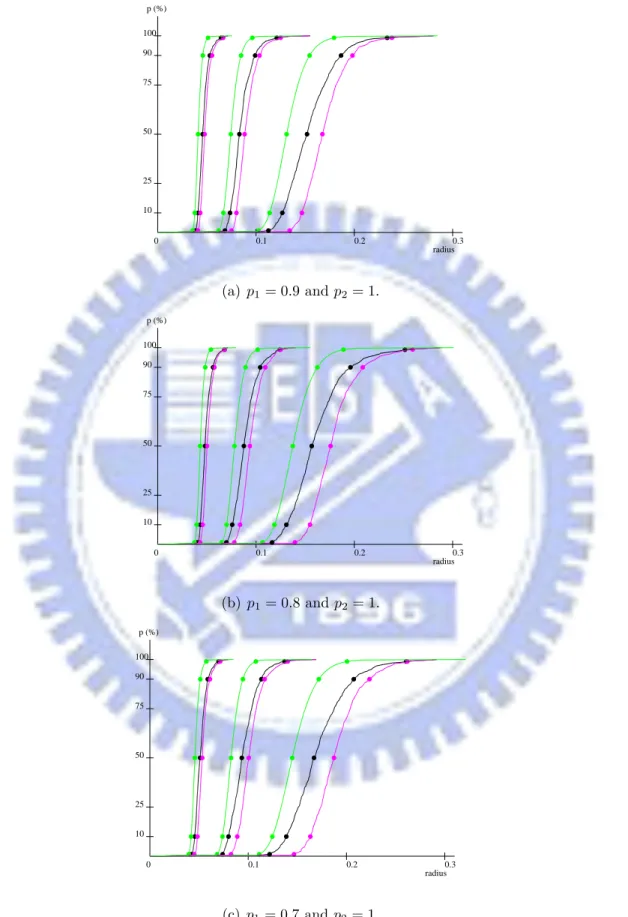
nodes, and solid lines are links between two nodes. Moreover, the white nodes represent the broken nodes. Figure 5.3(a) is the network without isolated nodes, and ab is the CTR for without isolated nodes and with length 0.132620. Figure 5.3(b) is the network with connectivity, and ab is the CTR for connectivity and with length 0.144876. Figure 5.4 illustrates the c.d.f. corresponding to p1 = 0.9, p1 = 0.8, and p1 = 0.7, respectively. The
p (%) 0 0.1 0.2 0.3 100 50 75 25 10 90 radius (a) p1= 0.9 and p2= 1. p (%) 0 0.1 0.2 0.3 100 50 75 25 10 90 radius (b) p1= 0.8 and p2= 1. p (%) 0 0.1 0.2 0.3 100 50 75 25 10 90 radius (c) p1= 0.7 and p2= 1.
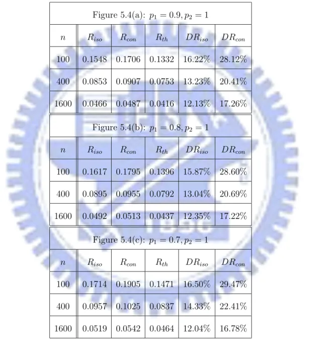
Table 5.2: The average CTR’s corresponding to Figure 5.4. Figure 5.4(a): p1 = 0.9, p2 = 1
n Riso Rcon Rth DRiso DRcon
100 0.1548 0.1706 0.1332 16.22% 28.12% 400 0.0853 0.0907 0.0753 13.23% 20.41% 1600 0.0466 0.0487 0.0416 12.13% 17.26%
Figure 5.4(b): p1 = 0.8, p2 = 1
n Riso Rcon Rth DRiso DRcon
100 0.1617 0.1795 0.1396 15.87% 28.60% 400 0.0895 0.0955 0.0792 13.04% 20.69% 1600 0.0492 0.0513 0.0437 12.35% 17.22%
Figure 5.4(c): p1 = 0.7, p2 = 1
n Riso Rcon Rth DRiso DRcon
100 0.1714 0.1905 0.1471 16.50% 29.47% 400 0.0957 0.1025 0.0837 14.33% 22.41% 1600 0.0519 0.0542 0.0464 12.04% 16.78%
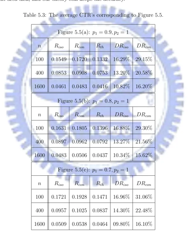
Besides generating points over an unit-area disk, we also run similar simulations over an unit-area square. The c.d.f. corresponding to p1 = 0.9, p1 = 0.8, and p1 = 0.7 are
illustrated by Figure 5.5. The average CTR’s and inaccuracies of Riso, Rcon, and Rth are
listed in Table 5.3. Basically, the results are similar to results of random point sets over an unit-area disk, and our theory still keeps the accuracy.
Table 5.3: The average CTR’s corresponding to Figure 5.5. Figure 5.5(a): p1 = 0.9, p2 = 1
n Riso Rcon Rth DRiso DRcon
100 0.1549 0.1720 0.1332 16.29% 29.15% 400 0.0853 0.0908 0.0753 13.20% 20.58% 1600 0.0461 0.0483 0.0416 10.82% 16.20%
Figure 5.5(b): p1 = 0.8, p2 = 1
n Riso Rcon Rth DRiso DRcon
100 0.1631 0.1805 0.1396 16.88% 29.30% 400 0.0897 0.0962 0.0792 13.27% 21.56% 1600 0.0483 0.0506 0.0437 10.34% 15.62%
Figure 5.5(c): p1 = 0.7, p2 = 1
n Riso Rcon Rth DRiso DRcon
100 0.1721 0.1928 0.1471 16.96% 31.06% 400 0.0957 0.1025 0.0837 14.30% 22.48% 1600 0.0509 0.0538 0.0464 09.80% 16.10%
p (%) 0 0.1 0.2 0.3 100 50 75 25 10 90 radius (a) p1= 0.9 and p2= 1. p (%) 0 0.1 0.2 0.3 100 50 75 25 10 90 radius (b) p1= 0.8 and p2= 1. p (%) 0 0.1 0.2 0.3 100 50 75 25 10 90 radius (c) p1= 0.7 and p2= 1.
In addition, we consider another scenario. Each node has probability p1 to stay in
waking state, and may switch to sleeping state independently with probability 1 − p1.
Nodes only do jobs in waking state, such as sending/receiving data, or being a member of the virtual backbone and relaying packet for other nodes. When in sleeping state, they do nothing but monitor a particular broadcasting channel, e.g. beacons in ZigBee networks [2]. Moreover, nodes in sleeping state need to have at least one waking neighbor to prevent from being isolated in the networks. For such networks, a node is isolated if it doesn’t have waking neighbors, and a network is connected if every nodes have at least one waking neighbors. Figure 5.6 shows two networks over the same 200 random nodes with defferent value of r’s deployed in an unit-area disk. Black nodes represent nodes in waking state, and white nodes represent nodes in sleeping state. Dotted lines are the listening links of white nodes to black nodes.
b a
(a) riso= |ab| = 0.129692.
a b
(b) rcon= |ab| = 0.172918.
Figure 5.6(a) is the network without isolated nodes, and ab is the longest edge and with length 0.129692 that is corresponding to the CTR for without isolated nodes, and the
r-disk graph is plotted with r = ka − bk. Figure 5.6(b) is the network with connectivity,
and ab is the longest edge and with length 0.172918 that is corresponding to the CTR for connectivity, and the r-disk graph is plotted with r = ka − bk. Note that the CTR can be contributed by a dotted line. The c.d.f. corresponding to p1 = 0.9, p1 = 0.8 and
p1 = 0.7 are illustrated by Figure 5.7.
The average CTR’s and inaccuracies of Riso, Rcon, and Rthare listed in Table 5.4. The
results are similar to those of the former scenario.
5.4
Networks with Bernoulli Nodes and Links
In the real world, wireless signals may be blocked or reflected by geographic barriers and buildings, and interfered by other singals. Thus, communication links is not avail-able everytime. So, besides unreliavail-able nodes, we consider networks with unreliavail-able links. Assume nodes may break down independently with probability 1 − p1, and links may be
down independently with probability 1−p2. Figure 5.8 shows the instance of two networks
over the same 200 nodes but with different value of r’s deployed in an unit-area disk with
p1 = 0.8 and p2 = 0.8. Black nodes represent well-functioned devices, and white nodes
represent failed ones. Edges denoted by solid lines between black nodes are up links, and edges denoted by dash lines are down links. Figure 5.8(a) is the network without isolated nodes, and ab is the longest edge and with length 0.097235 that is corresponding to the CTR such that every black nodes have at least one solid edge, and the graph is plotted
p (%) 0 0.1 0.2 0.3 100 50 75 25 10 90 radius (a) p1= 0.9 and p2= 1. p (%) 0 0.1 0.2 0.3 100 50 75 25 10 90 radius (b) p1= 0.8 and p2= 1. p (%) 0 0.1 0.2 0.3 100 50 75 25 10 90 radius (c) p1= 0.7 and p2= 1.
Table 5.4: The average CTR’s corresponding to Figure 5.7. Figure 5.7(a): p1 = 0.9, p2 = 1
n Riso Rcon Rth DRiso DRcon
100 0.1557 0.1704 0.1346 15.71% 26.62% 400 0.0860 0.0910 0.0759 13.28% 19.83% 1600 0.0468 0.0486 0.0418 11.86% 16.24%
Figure 5.7(b): p1 = 0.8, p2 = 1
n Riso Rcon Rth DRiso DRcon
100 0.1662 0.1815 0.1427 16.42% 27.15% 400 0.0918 0.0972 0.0806 13.93% 20.70% 1600 0.0501 0.0519 0.0444 12.95% 16.98%
Figure 5.7(c): p1 = 0.7, p2 = 1
n Riso Rcon Rth DRiso DRcon
100 0.1786 0.1936 0.1526 17.06% 26.88% 400 0.0980 0.1032 0.0861 13.81% 19.81% 1600 0.0537 0.0557 0.0474 13.20% 17.34%
b a
(a) riso= |ab| = 0.097235.
b a
(b) rcon= |ab| = 0.135864.
Figure 5.8: The r-disk graph with unreliable nodes and links.
with r = ka − bk. Figure 5.8(b) is the network with connectivity, and ab is the longest edge and with length 0.135864 that is corresponding to the CTR such that black nodes and solid edges form a connected graph, and the graph is plotted with r = ka − bk. Figure 5.9 illustrates the c.d.f. of CTR’s corresponding to p1 = 0.9, and respectively p2 = 0.9,
p2 = 0.8, and p2 = 0.7.
The average CTR’s and inaccuracies of Riso, Rcon, and Rth are listed in Table 5.5.
In addition, we consider another scenario in which every nodes independently stay in waking state with probability p1 and in sleeping state with probability 1 − p1, instead
of breaking down. For such networks, a node is isolated if it doesn’t have an up link connecting to black node, and a network is connectied if awake nodes are connected by solid edge and every sleeping nodes have at least one solid edge. Figure 5.10 illustrates the c.d.f. of CTR’s corresponding to p1 = 0.9, and respectively p2 = 0.9, p2 = 0.8, and
p (%) 0 0.1 0.2 0.3 100 50 75 25 10 90 radius (a) p1= 0.9 and p2= 1. p (%) 0 0.1 0.2 0.3 100 50 75 25 10 90 radius (b) p1= 0.8 and p2= 1. p (%) 0 0.1 0.2 0.3 100 50 75 25 10 90 radius (c) p1= 0.7 and p2= 1.
Table 5.5: The average CTR’s corresponding to Figure 5.8. Figure 5.9(a): p1 = 0.9, p2 = 0.9
n Riso Rcon Rth DRiso DRcon
100 0.1619 0.1753 0.1404 15.33% 24.88% 400 0.0902 0.0943 0.0794 13.58% 18.78% 1600 0.0494 0.0509 0.0438 12.81% 16.10%
Figure 5.9(b): p1 = 0.9, p2 = 0.8
n Riso Rcon Rth DRiso DRcon
100 0.1704 0.1823 0.1489 14.43% 22.42% 400 0.0963 0.0991 0.0842 14.33% 17.69% 1600 0.0522 0.0532 0.0465 12.30% 14.50%
Figure 5.9(c): p1 = 0.9, p2 = 0.7
n Riso Rcon Rth DRiso DRcon
100 0.1859 0.1945 0.1592 16.79% 22.22% 400 0.1024 0.1048 0.0900 13.71% 16.44% 1600 0.0563 0.0570 0.0497 13.43% 14.68%
p2 = 0.7.
The average CTR’s and inaccuracies of Riso, Rcon, and Rth are listed in Table 5.6.
Table 5.6: The average CTR’s corresponding to Figure 5.10. Figure 5.10(a): p1 = 0.9, p2 = 0.9
n Riso Rcon Rth DRiso DRcon
100 0.1651 0.1778 0.1419 16.41% 25.35% 400 0.0911 0.0950 0.0801 13.74% 18.62% 1600 0.0497 0.0507 0.0441 12.63% 14.98%
Figure 5.10(b): p1 = 0.9, p2 = 0.8
n Riso Rcon Rth DRiso DRcon
100 0.1765 0.1856 0.1505 17.32% 23.35% 400 0.0964 0.0991 0.0849 13.55% 16.73% 1600 0.0525 0.0534 0.0468 12.30% 14.07%
Figure 5.10(c): p1 = 0.9, p2 = 0.7
n Riso Rcon Rth DRiso DRcon
100 0.1889 0.1966 0.1609 17.43% 22.21% 400 0.1039 0.1057 0.0908 14.44% 16.49% 1600 0.0568 0.0573 0.0500 13.60% 14.59%
p (%) 0 0.1 0.2 0.3 100 50 75 25 10 90 radius (a) p1= 0.9 and p2= 1. p (%) 0 0.1 0.2 0.3 100 50 75 25 10 90 radius (b) p1= 0.8 and p2= 1. p (%) 0 0.1 0.2 0.3 100 50 75 25 10 90 radius (c) p1= 0.7 and p2= 1.
5.5
Secure Wireless Networks
The last simulations are for the m-composite key predistribution scheme [19] [20] [21]. In secure networks with key pool size K and key ring size k, at least m common keys are required for each pair of nodes to establish secured links. For example, Figure 5.11 is two secure networks over the same 200 random nodes but with defferent value of r’s.
a b
(a) riso= |ab| = 0.106341.
b a
(b) rcon= |ab| = 0.118285.
Figure 5.11: The secure networks with K = 40, k = 10, and m = 2.
Two nodes at the same position in Figure 5.11(a) and Figure 5.11(b) respectively own the same key ring which are randomly drawn from the key pool. Solid lines are secured links, and dashed lines are unsecured links. The edge ab marked by red line is corresponding to the CTR of each network. In the simulations, we assume K = 40 and
k = 10. To focus our attention on the effect of the key predistribution scheme, we assume
all nodes are active, i.e. p1 = 1. Figure 5.12 illustrates the c.d.f. of CTR’s corresponding
p (%) 0 0.1 0.2 0.3 100 50 75 25 10 90 radius (a) m = 1. p (%) 0 0.1 0.2 0.3 100 50 75 25 10 90 radius (b) m = 2.