環物影片產生及應用技術之研究

I

國

立

交

通

大

學

資訊科學系

博

士

論

文

環物影片產生及應用技術之研究

New Techniques for Production and Application of Object Movies

研 究 生：蔡玉寶

指導教授：施仁忠 教授

洪一平 教授

II

環物影片產生及應用技術之研究

New Techniques for Production and Application of Object Movies

研 究 生：蔡玉寶 Student：Yu-Pao Tsai

指導教授：施仁忠教授 Advisors：Dr. Zen-Chung Shih

洪一平教授

Dr. Yi-Ping Hung

國 立 交 通 大 學

資 訊 科 學 系

博 士 論 文

A Dissertation

Submitted to Department of Computer and Information Science College of Electrical Engineering and Computer Science

National Chiao Tung University in partial Fulfillment of the Requirements

for the Degree of Doctor of Philosopy

in

Computer and Information Science June 2007

Hsinchu, Taiwan, Republic of China

i

環物影片產生及應用技術之研究

學生: 蔡玉寶 指導教授: 施仁忠教授

洪一平教授

國立交通大學資訊科學學系﹙研究所﹚博士班

摘 要

由於環物影片(Object Movies)在建置上相當簡單以及能產生相片品質的成像結 果，因此環物影片目前已是一種非常通用的方法來表現可互動的三維物體。雖然環物影 片已成功地被應用在不同的領域，但關於產生高品質環物影片的技術以及更具有開創性 應用的技術都有待研究開發。 本論文提出一些方法來產生高品質的環物影片以及展示一些利用環物影片來表現 三維物體的應用。首先，我們提出一個環物影片拍攝架的挍正方法並提供一個視覺化的 界面幫助使用者根據計算結果來調整拍攝架。實驗顯示利用此校正方法，只需取得12張 校正物的影像便可以得到任一視角的精確相機參數。接著，我們提出環物影片背景去除 的方法。該方法最主要的好處是使用者的介入非常地少。更確切地說使用者只需從自動 去背景後的影像中選擇足夠好的結果，該方法便能自動地將這些正確的資訊傳遞到其它 的影像並修正去背結果。在傳遞的過程中，該方法利用選擇的影像重建該三維物體的三 維幾何形狀，再投影到其它的影像上產生物體的剪影以協助自動去背方法產生更好的去 背結果。實驗顯示，透體這剪影資訊可以明顯地降低去背結果的誤差並能有效地抵抗雜 訊的影響。另外，一個新的三維重建方法被提出來從環物影片之中重建出該物體的三維 資訊。相較之前的方法，該方法所產生的三維模型可以保留住更多的細節部份而且其剪 影會和原始輸入的剪影影像相吻合。最後，我們延續之前環場環物整合技術的研究，提 出可將立體環物整合到立體環場的方法。使用者可以透過所提供的系統可以整合立體環

ii

場環物建置出一個非常逼真的互動環境，並可直接瀏覽該虛擬環境以及觀看立體環物。 經由這樣的互動環境使用者可以透過立體視覺體驗到更真實的3D感受。

iii

New Techniques of Production and Application of Object Movies

Student: Yu-Pao Tsai Advisors: Dr. Zen-Chung Shih

Dr. Yi-Ping Hung

Department﹙Institute﹚of Computer and Information Science

National Chiao Tung University

Abstract

Object movie (OM) is a conventional approach for modeling and rendering interactive 3D objects because of its simplicity in production and its photorealistic presentation of objects. Although OMs have been successfully adopted in many applications, the techniques for production and application of OMs must still be enhanced if high-quality and efficient OMs are desired.

This work proposes some methods for generating high quality OMs, and demonstrates some applications using generated OMs to present the 3D objects. First, a method for calibrating the motorized object rig is presented, and a visual tool is introduced to adjust the axes of the motorized object rig. The distances among all the three axes of the motorized object rig can be minimized after adjustment, and more reliable camera parameters can be obtained after the calibration process. Experimental results indicate that highly accurate parameters can be obtained from only 12 images. Second, an image segmentation method is proposed to remove the backgrounds of OMs. The major advantage of the proposed method is it can propagate the successful segmentation results from some selected images to the whole OM. The

iv

new OM segmentation method extracts a 2D shape from the reconstructed 3D model and uses the 2D shape to remove the background from the foreground object. This work demonstrates that the proposed method can significantly improve OM segmentation. Third, a novel approach is proposed to reconstruct high quality 3D models from OMs. The silhouettes and detail features of reconstructed 3D model are successfully preserved. Finally, previous work on augmented panoramas is extended to augmented stereo panoramas. This work develops an interactive system that allows the user to integrate stereo OMs into a stereo panorama, and interactively browses the augmented stereo panorama. To generate stereo OMs, the 3D models reconstructed from monocular OMs are rendered. The proposed method takes less than half of the processing time, including acquisition and segmentation, than traditional approaches, which take two separate sets of OMs. The proposed interactive system provides the users with two approaches to determine the reference frames where the object is inserted in a stereo panorama. The left view and the right view are rendered separately after determining the reference frames. For each view, the background layer is first rendered, followed by the shadow and the object layers. A user can directly rotate and translate the stereo object movie of interest by browsing the augmented panorama. The augmented stereo panoramas provide users with more persuasive interaction with better depth perception.

v

Content

摘        要 ... I  ABSTRACT ... III  CONTENT ... V  LIST OF FIGURES ... VII  LIST OF TABLES ... XII  CHATPER 1  INTRODUCTION ... 1  1.1.  MOTIVATION _... 1 

1.2.  REVIEW OF RELATED WORK _... 4 

1.3.  ORGANIZATION OF THIS THESIS _... 8 

CHATPER 2  OBJECT RIG CALIBRATION ... 9 

2.1.  ESTIMATION OF CAMERA PARAMETERS _... 10 

2.2.  COMPLETELY AND PARAMETER CONTINUOUS (CPC)KINEMATIC MODEL_... 11 

2.3.  KINEMATIC CALIBRATION USING THE CPCMODEL _... 13 

2.4.  EXPERIMENTAL RESULTS OF CALIBRATION _... 18 

CHATPER 3  BACKGROUND REMOVAL ... 22 

3.1.  INITIAL LABELING _... 25 

3.2.  LABEL UPDATING WITH MOTION VECTORS _... 28 

3.3.  LABEL UPDATING WITH SHAPE PRIORS _... 32 

3.4.  EXPERIMENTAL RESULTS OF BACKGROUND REMOVAL _... 36 

CHATPER 4  OBJECT MOVIE‐BASED 3D RECONSTRUCTION ... 44 

4.1.  VOLUMETRIC GRAPH CUTS _... 44 

4.2.  OUR APPROACH _... 49 

4.3.  EXPERIMENTAL RESULTS OF 3DRECONSTRUCTION _... 55 

CHATPER 5  AUGMENTED STEREO PANORAMAS ... 61 

5.1.  GENERATION OF STEREO PANORAMAS _... 61 

5.2.  GENERATION OF STEREO OBJECT MOVIES _... 63 

5.3.  AUGMENTING STEREO PANORAMAS WITH STEREO OMS _... 64 

5.4.  EXPERIMENTAL RESULTS OF AUGMENTED STEREO PANORAMAS _... 66 

vi

REFERENCES ... 71 

APPENDIX ... 76  SINGULARITY-FREE LINE REPRESENTATION _... 76 

vii

List of Figures

Fig. 1. Motorized object rig – AutoQTVR. ... 2 

Fig. 2. Motorized object rig – Kaidan Magellan™ 2500. ... 2 

Fig. 3. Processing Flowchart of Calibration ... 10 

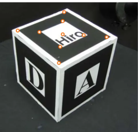
Fig. 4. The calibration object, called physical control cube (PCC), and the extracted feature points used to obtain intrinsic camera parameters. ... 11 

Fig. 5. The schematic of motorized object rig. ... 14 

Fig. 6. The OM of the toy shark before calibration. (a) shows the estimated relation among 3 axes, and (b) shows the OM of the toy shark. The cross markers indicate the center of images. ... 20 

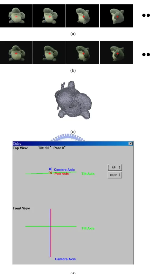
Fig. 7. The result of the toy shark experient. (a) shows some images of the OM of the toy shark after calibration, while (b) shows that after centralization. (c) shows the Visual Hull of the shark, and (d) shows the estimated axes after calibration. ... 21 

Fig. 8. Part of the two different equi-tilt sets before applying the OM segmentation method. Except for leftmost two images in the figure, the remainder of the images in this thesis are cropped in order to show more examples. ... 23 

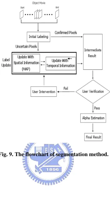
Fig. 9. The flowchart of segmentation method. ... 25 

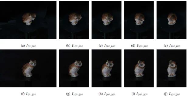
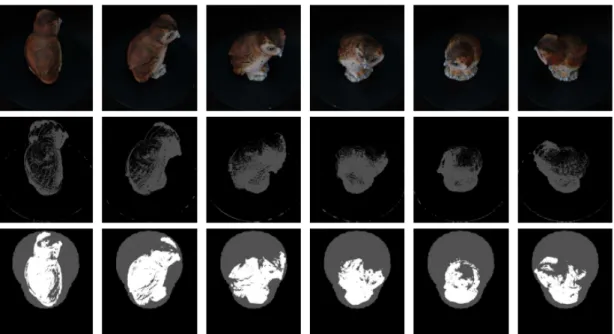
Fig. 10 The top row shows a portion of the input image sequence taken from an equi-tilt set of the pottery owl OM. For all the images in the middle and bottom rows, the black pixels correspond to the classified background regions. The foreground regions are colored white, and the unknown regions are colored gray. The middle row shows the corresponding result during the B-labeling for each image. Notably, to filter out the incorrectly classified pixels and obtain the global background mask used during F-labeling, label consistency and mathematical morphology are used as shown in Fig. 11. Finally, the bottom rows shows the generated trimap for each image that is used to activate the graph cut image segmentation. ... 27 

Fig. 11. (a) The result including the label consistency concept is included; (b) The global background mask obtained by applying the mathematical morphology on (a). ... 28 

Fig. 12. 2D spatial graph construction example. ... 29 

Fig. 13. The worms of the uncertain pixels i1 and i2 ... 32 

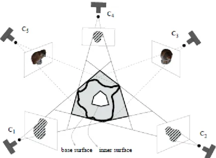
Fig. 14. The process flowchart of the new system. ... 35  Fig. 15. C1, C2, and C4 denote the views adopted to built the visual hull. Notably, the true

surface of the object is assumed to be between the base and inner surfaces. Although the segmentation results of C3 and C5 are poor, they can be improved by incorporating

viii

the projection of the reconstructed model into the graph cut image segmentation algorithm. ... 36  Fig 16 The top row shows a portion of the input image sequence taken from an equi-tilt set

of the pottery owl OM. For all the images in the middle and bottom rows, the black pixels correspond to the classified background regions. The foreground regions are colored white, and the unknown regions are colored gray. The middle row shows the corresponding result during the B-labeling for each image. Finally, the bottom rows show the generated trimap for each image that is used to activate the graph cut image segmentation. ... 39  Fig. 17. The results of the automatic initial segmentation corresponding to the image

sequence shown in Fig 16. The three images on the left show the segmentation results that should be selected for the 3D reconstruction, while the others shows results that should be excluded and refined in the next run. The red circles denote the noticeable segmentation errors in each image. ... 40  Fig. 18. The top row shows a portion of an equi-tilt set for the toy house OM. The middle

row shows the trimap labeling result for each image. Finally, the bottom row shows the results of the automatic initial segmentation. The red circles indicate the noticeable segmentation errors in each image, to be rectified in the next run. ... 40  Fig. 19. The rectification of the segmentation errors for the pottery owl in Fig. 17 and the

toy house in Fig. 18. Trimaps (top row): the projection of the reconstructed model is colored white, and serves as the foreground hard constraints together with the previously generated trimap. Refinement (bottom row): the refinement of the segmentation result is shown for each image. ... 41  Fig 20. The first row shows six consecutive images in an equi-tilt set of the pottery cat OM.

The second row shows the result of trimap labeling. The third row shows the result of the automatic initial segmentation. In the fourth row, the projection of the reconstructed 3D model provides the information on regions that is quite difficult to obtain by the methods based on color and contrast alone. The last row shows the refinement of the segmentation result by using shape priors. ... 41  Fig. 21. The Armadillo that is the 3D model adopted to generate the synthetic data. ... 42  Fig. 22 Mean segmentation errors on the synthetic data. The image size is 800 x 600. In the

experiments, the 3D shape was reconstructed by randomly selecting ground truth images. The shape prior 1 was learnt by using 10 images, and the shape prior 2 was learnt by 20 images. ... 42  Fig. 23. The first row shows six consecutive images in an equi-tilt set of the Armadillo OM.

The second row shows the result of trimap labeling. The third row shows the result of the automatic initial segmentation. In the fourth row, the projection of the reconstructed 3D model provides the information on regions that is quite difficult to

ix

obtain by the methods based on color and contrast alone. The fifth row shows the refinement of the segmentation result by using shape priors. The last row shows the comparison between the segmentation results produced by the proposed method and the ground truth. The red solid lines denote the contours of the ground truth, and the

green dot lines denote the segmentation results produced by the proposed method ... 43 

Fig. 24. Illustration of volumetric graph cuts algorithm. (a) Graph cuts algorithm is used to find the Smin surface between Sbase and Sin in volumetric graph cuts. (b) xi and xj are the neighbor voxels. The edge weight between these two voxels is represented as wij and the edge weight between voxels and source node is represented as wb. h means the length between two voxels. ... 47 

Fig. 25 Two cases that cause errors may occur in volumetric graph cuts. Because of the shorter cut property of volumetric graph cuts, Concavity-Convex feature will be flattened in volumetric graph cuts. ... 48 

Fig. 26. Silhouette images. (a) is the input silhouette image for 3D reconstruction. (b) is the silhouette image generated from the reconstruction model using volumetric graph cuts algorithm. ... 48 

Fig. 27. The comparison between silhouette images shown in Fig. 26. The unmatched regions are colored in red and green. ... 49 

Fig. 28. The broken ears is caused by not considering the silhouette information in volumetric graph cuts. ... 49 

Fig. 29. The flowchart of our approach. This approach contains two phases. In the first phase, a silhouette-preserved model is generated by a silhouette-preserved volumetric graph cuts algorithm. Then, the result of phase 1 is refined by gradient descent in phase 2. ... 50 

Fig. 30. Silhouette-preserved volumetric graph cuts algorithm. Orange circle: the 3D object to be reconstructed. Purple grid: The voxels labeled “IN Object” after volumetric graph cuts. Red grid: The voxels have to increase edge weights to match the silhouettes. ... 53 

Fig. 31. A silhouette image projected from the reconstructed 3D model using the silhouette-preserved volumetric graph cuts. ... 53 

Fig. 32 Comparison between silhouette images shown in Fig. 31 and Fig. 26 (a). ... 53 

Fig. 33. The reconstructed 3D model after phase 1. Notably, The broken ears are fixed. ... 54 

Fig. 34 The meaning of symbols in (50) ... 55 

Fig. 35. The reconstructed model of the toy house by using the volumetric graph cuts algorithm without imposing the DMA constraint. The ballooning term is increased gradually from left to right. The figure indicate that reconstructing the toy house is a difficult task without the DMA constraint. ... 57 

x

Fig. 36. Visualization and comparison of the 3D reconstruction algorithm. Both (b) and (c) are taken from a cross-section of the visual hull for the toy house, which is shown in (a). The golden voxels correspond to the base surface in all three images. The cyan voxels denote the inner surface, which is parallel to the base surface. Additionally, the voxels in VA are also colored cyan in (c). The photo-consistency scores between the base and inner surfaces are shown, where the darker region indicates a better photo-consistency. Additionally, the line within the base and inner surfaces represents the reconstructed surface of the object. In (b), without the DMA constraint, although the reconstructed surface passes through the worse photo-consistency regions, the integral of the energy on the entire surface is lower. Consequently, the protrusive part (i.e., the tower of the house) is flattened incorrectly. The image in (c) shows the correctly reconstructed surface for the same portion of the object with the DMA constraint. ... 57  Fig. 37. Image (a) shows the visual hull generated from the available silhouettes of the toy

house to act as the base surface in the algorithm; (b) the DMA of the visual hull that is considered to be an approximate DMA of the toy house. Images (c)-(h) show the reconstructed model from three different viewpoints of the toy house, together with the images captured at similar viewpoints. ... 58  Fig. 38. (a) The visual hull of the pottery owl. (b) The DMA of the visual hull. (c) An

example image of the pottery owl MVI. (d) The reconstructed model of the pottery owl by using our method. ... 58  Fig. 39 The reconstructed owl models. (a) The result of phase one. (b) The result of phase

two. ... 59  Fig. 40 The reconstruction results of the bunny model. (a) The result of traditional

volumetric graph cuts algorithm (b) The result of phase one (c) The result of phase two (b) The ground truth. ... 59  Fig. 41 The reconstructed buddha models. (a) The result of traditional volumetric graph cuts.

(b) The result of phase 1. (c) the result of phase 2 (d) The ground truth. ... 59  Fig. 42 Comparison between our result and original image. Left is the original image and

the right is the result reconstructed by our method. ... 60  Fig. 43. A diagram shows the idea to create a stereo panorama using a video camera. ... 62  Fig. 44 (a) The original OM images. (b) Our rendering results of binocular views... 64  Fig. 45. The UI allows users to integrate stereo OMs into a stereo panorama in 3D mode. .... 66  Fig. 46. Illustration of casting shadow for an object movie. ... 66  Fig. 47: Stitching result of a stereo panorama. ... 67  Fig. 48: Result of the augmented panorama with a stereo OM. (a) shows the rendered left

xi

Fig. 49 Rotating the OM in the augmented stereo panorama. (a) and (c) are the left views. (b) and (d) are the right views. ... 67

xii

List of Tables

 

Table 1. Processing time and accuracy of the calibration processing ... 19   

1

Chatper 1

Introduction

1.1. Motivation

Modeling and rendering photorealistic 3D objects are significant tasks in computer graphics. Two conventional techniques are the geometry-based and the image-based approaches. The geometry-based approach first constructs 3D models of real world objects then generates the results by rendering the 3D models with attached textures. This approach provides good interactivity, but the 3D models to be constructed, which is a tedious process. In contrast, the image-based approach uses real images for interactive displaying and browsing. It provides photo-realistic visual effects, and its rendering speed is independent of the complexity of the scenes or objects.

Many methods have been proposed for image-based modeling and rendering. Object movie (OM) proposed by Apple Inc. is a conventional approach because of its simplicity in acquisition and its photorealistic ability to present the 3D objects. OM has recently been widely adopted in many applications, e.g., e-commerce, digital archive, digital museum [32], etc. An OM is a set of images taken from different perspectives around a 3D object. Fig. 1 and Fig. 2 show two different motorized object rigs. The OM can be treated as an interactive video of the 3D object after acquisition. Each image in an OM is associated with a pair of distinctive pan and tilt angles of the viewing direction, allowing a particular image to be chosen and shown on screen according to the user’s viewing direction, which is generally specified by controlling mouse motion. Users can thus interactively rotate the virtual artifacts arbitrarily, and freely

2 manipulate the object.

Although OMs have been successfully used in many applications, the techniques for producing OMs still need to be improved if high-quality and efficient OMs are desired. This work investigates the methods of production and applications of high-quality OMs.

The motorized object rig, AutoQTVR, developed by Texnai Inc., was adopted to acquire the OMs. The motorized object rig is a computer-controlled 2-axis omniview shooting system, as shown in Fig. 1. It has two rotary axes, the pan-direction object rotator and the tilt-direction camera arm rotator. For convenience, these rotation axes of the rotators are called the tilt and the pan axes, respectively.

Fig. 1. Motorized object rig – AutoQTVR.

Fig. 2. Motorized object rig – Kaidan Magellan™ 2500.

3

rotation axes and the optical axis of the camera, as shown in Fig. 1. Otherwise, the acquired OM would have a bizarre rotation effect when it is browsed. Consequently, to acquire high quality OMs that rotate smoothly, the three axes should first be made to intersect at a common point, Cs.

However, since the optical axis of the camera is invisible, aligning these three axes is inherently a difficult problem. This work develops a method for calibrating a motorized object rig to facilitate the acquisition of OMs, and for improve the accuracy of camera parameters, which can be used for different subsequent tasks, e.g., 3D reconstruction, background removal, and stereo OM generation.

To enhance the rendering results, or to integrate OMs into a new background, the background must be efficiently and effectively removed from the foreground object. However, this is a challenging task. Additionally, another task requires OM segmentation is 3D reconstruction using captured OMs. However, as is well known, OM segmentation is a more tedious and expensive task than the acquisition of the OM as mentioned above. In our experience, segmenting the images manually would take more than 30 man-hours, because an OM generally contains hundreds of images. Additionally, the OM segmentation task can become very time-consuming and burdensome for stereo object movies [9].

Yielding two distinct foreground and background color distributions can obviously mitigate the difficulty of OM segmentation. Blue-screen and green-screen matting have been widely adopted in movie production to achieve this purpose. However, a black screen is preferable for acquiring the OM to prevent the object from reflecting the blue or green light, particularly in the domain of digital archives and digital museums. A black screen frequently results in ambiguously shadowed regions that can significantly increase the difficulty of OM segmentation, such that even a patient expert might become tired of the segmentation. Therefore, the usability of the designed OM segmentation method should be examined in terms of computational expense, accuracy of the segmentation result and amount of user intervention. This work devises a new image segmentation method to help the user obtain a quality OM

4 segmentation result in less than one man-hour.

Many applications require 3D geometry model to perform 3D processing, e.g., shadow generation, collision detection, lighting and novel view generation, for to enhance rendering results and visual effects. This work investigates how to reconstruct 3D models from OMs to improve the applications of OMs. Given the camera parameters and silhouette images, some methods [28][49][62][22] have been proposed to recover the 3D model from multi-view images. To the best of our knowledge, the graph cuts based methods [62][22] can produce the better results than other methods[28][49]. However, the graph-cut-based methods do not preserve either concavity-convex features or silhouettes are not preserved. To improve the 3D model, a two phase approach is proposed to deal with these problems in this thesis.

Since binocular vision provides the human depth perception of 3D objects, with stereo vision, the viewer can see where objects are in relation to them with high precision, especially when those objects are moving toward or away from them. To benefit from human binocular visions, this work extends the work on augmented panoramas [25] to augmented stereo panoramas. Once the 3D modes are reconstructed, stereo OMs can be generated from monocular OMs with the help of the 3D model. After producing high-quality OMs, this work develops an interactive system that allows the user to integrate stereo OMs into a stereo panorama, and to interactively browse the augmented stereo panorama. A user can directly browse the stereo OMs of interested by navigating in the augmented stereo panorama with a stereoscopic display. With augmented stereo panoramas, the user can enjoy more persuasive interaction with better depth perception.

1.2. Review of Related Work

Virtual reality systems involve two major classes of technique, i.e., geometry-based and image-based rendering. In geometry-based methods, a complete 3D model of the environment,

5

including all the objects within the virtual world, is constructed and rendered to simulate the virtual world. Conversely, image-based methods, collections of images taken from different viewpoints of the environment are used to generate novel views of the virtual world. Both approaches have their own advantages and weaknesses. However, image-based methods have become increasingly popular, because they can easily be applied to construct high-quality and photorealistic environments. Shum et al. [56] performed a thorough survey of image-based rendering techniques, and classified the techniques into three categories according to the amount of geometric information used: rendering without geometry[12][29][54], rendering with implicit geometry (i.e. correspondence)[11][19] and rendering with explicit geometry (either with approximate or accurate geometry)[7][51]. Light Field Rendering [29] and Lumigraphs [19] are two famous methods, but their large memory requirements make them impractical for real applications, especially those requiring Internet transmission. Conversely, OM has a smaller storage requirement than those methods. The OM approach can be classified into the first class, rendering without geometry, because it does not need 3D information when rendering OMs. OM has recently become the most popular approach to modeling and rendering the 3D objects, and has been adopted in many applications. This work investigate the techniques for producing high quality OMs including object movie rig calibration, OM segmentation, stereo OMs generation, and 3D reconstruction. The related work is discussed as follows.

As described in Section 1.1, the aim of the rig calibration is to ensure that the pan-, the tilt- and the optical- axes intersect at a common point, Cs. Since a camera is mounted on the object

movie rig, it can be used to perform the calibration, which can be considered as a pose estimation problem. The problem is widely studied in robotic motion and automatic industry [35][42]. A camera can be adopted in a robot system to determine the robot pose from the camera extrinsic parameters, as is well known. Camera calibration is widely discussed. Calibration methods fall into two categories. The first category is self-calibration, in which the

6

camera parameters are estimated without any reference object, by moving a camera in a static scene [21][39]. However, many parameters need to be estimated, making reliable results hard to obtain. The other calibration methods are estimation with a reference object. Calibration is performed by observing a calibration object whose geometry in 3D space is known with very high precision [58]. In this thesis, the motorized object rig is formulated with the kinematic model. Denavit and Hartenberg [16] developed a notation for assigning orthonormal coordinate frames to a pair of adjacent links in an open kinematic chain. However, parameter jumps occur when two consecutive joint axes change from parallel to almost parallel. Zhuang et al. [69] proposed a complete and parametrically continuous (CPC) kinematic model to avoid this situation.

To our knowledge, OM segmentation is currently performed entirely by the artists. These experts mainly manipulate some industrial interactive tools (e.g., magic wand and intelligent scissors from Adobe Photoshop [1]) to remove the backgrounds of each image individually. The work flow does not utilize any information between images captured in neighboring viewing directions, and consequently is very expensive. Unfortunately, background removal in the OM has not been widely investigated, so OM segmentation is an obstacle to the spreading of image-based objects.

Interactive background removal tools have been developed for many years because of their practical importance. Such tools include magic wand [1], intelligent scissors, [40][41][26] Bayesian matting [13], graph-cut-based image segmentation [6][47][31][17][11], and interactive matting based on belief propagation [64]. The color information (e.g., foreground and background color model) and contrast information (e.g., gradient and edge strength) are usually exploited to achieve the goal. The most popular of these methods is probably graph-cut-based image segmentation. The remaining of the image are automatically classified as the foreground or background immediately after a user manually provides foreground and background hard constraints on the image. These approaches are often quite successful for

7

single-image segmentation, but hard to apply to the OM segmentation due to the endless drudgery of manually specifying hard constraints on each image of the OM individually.

OM background removal is a specific type of video object segmentation. Some automatic methods for video object segmentation have been proposed [44][36], but are not always able to extract the desired video objects. Some researchers have proposed semi-automatic methods that allow user interaction to improve the accuracy of results [20][36][38][67]. Although many approaches have been proposed to deal with video object segmentation, none of these are devoted to object movie segmentation.

Generating stereo OMs from monocular ones is a novel view generation problem, which can be intuitively solved by image morphing [4][48]. Since it does not consider any 3D information, it may produce unexpected effects. View morphing [50] utilizes additional 3D information, such as epiploar geometry and camera parameters, to eliminate the unexpected effects. Moreover, image morphing and view morphing require corresponding features on the original images. However, obtaining good corresponding features is also an open problem. Another approach tries to reconstruct a geometric model of the object according to the consistency with the image information. A calibrated laser projector and a calibrated camera can be used to reconstruct 3D surface [59]. However, laser scanner devices are expensive. Another methods [18][61][37], photometric stereo, can recover high-quality 3D models. To utilize these methods, the lights must be conscientiously and carefully controlled, which is impractical for many applications. Passive methods have been developed for more practical purposes. Laurentini [28] proposed a stable method, called visual hull, to reconstruct a 3D surface using silhouette information. However, his method cannot recover the concavity features of the 3D objects. Seitz and Dyer [49] proposed an improved method that considers voxel colors from different views in order to carve the voxels outside of the true surface. However, the method has a problem in that the surface points are dispersed. Vogiatzis et al. [62] recently proposed a graph-cut-based method, called volumetric graph cuts, to solve this

8

problem. Because graph cuts algorithm prefers shortest cut, the volumetric graph cuts has the problems that concavity-convex features and silhouettes cannot be preserved. Tran and Davis [57] tried to solve these problems with silhouette constraints. Their method sets hard constraints on some verified surface voxels. It works well for some cases, but does not solve the problems completely.

1.3. Organization of this Thesis

This thesis investigates the techniques of producing high-quality OMs, including object movie rig calibration, OM segmentation, and stereoscopic OMs generation. Chapter 2 presents a calibration method for object movie rigs to help users to acquire high quality OMs, and to obtain camera parameters. Chapter 3 describes two segmentation methods for removing the backgrounds of OMs. The objective of the proposed segmentation method is to minimize the user intervention. The first method utilizes motion vectors to propagate the corrected information to other frames containing segmentation errors. It works well for most cases, but requires much user intervention for some cases due to error motions. Therefore, the second method is proposed to propagate the corrected information efficiently by previously learning shape priors. Chapter 4 presents a novel 3D reconstruction approach to obtain high-quality 3D models from OMs. Chapter 5 describes a novel method, called augmented stereoscopic panoramas, to augment stereo panoramas with stereo OMs. With augmented stereo panoramas, the user can enjoy more persuasive interaction with better depth perception. A conclusion is given in Chapter 7.

9

Chatper 2

Object Rig Calibration

In this chapter, we describe a method for assisting the user to acquire high-quality OMs, and fast obtain the camera parameters of images in OMs. The camera parameters can be used in many applications. In this work, we will use the parameters to perform background removal in Chapter 3, 3D reconstruction and novel view generation in Chapter 4.

Fig. 3 shows the processing flowchart of the proposed calibration method. To calibrate the motorized object rig, we first use the camera mounted on the AutoQTVR to capture some feature points, whose 3D positions are known beforehand. The 2D and 3D positions of the feature points are used to estimate the intrinsic and extrinsic camera parameters. In our experiments, the calibration object, called the physical control cube (PCC) [24], is shown in Fig. 4. With the estimated extrinsic camera parameters, we can reconstruct the kinematic model of the rig. Then, we apply a simple and practical model, completely and parameter continuous (CPC) model [1][69], to formulate the relation among the three axes. Finally, we provide a visual tool showing the axes for users to adjust the motorized object rig. If the intersections of the rays are not close enough, the user can adjust the motorized object rig according to the estimated result, and then the axes will be estimated again. The whole process will be repeated until the intersections of the rays are close enough. After calibration, reliable extrinsic parameters of the camera will be available with the kinematic model.

10

Fig. 3. Processing Flowchart of Calibration

2.1. Estimation of Camera Parameters

We adopt the method proposed by Zhang [66] to estimate the intrinsic camera parameters. The method performs camera calibration with at least two images of a known planar pattern captured at different orientations.

On the other hand, we adopt the method presented in [9] and [24] to estimate the extrinsic camera parameters, by first using the method proposed by Kato et al. [27] to obtain a set of

Obtain a set of images of the calibration object

Estimate the intrinsic parameters

Estimate the extrinsic parameters (Initial values obtained by using ARToolkit library and refined by

ICP) +

OpenCV Library

Pan and Tilt angles of

the captured images Estimate the relation among axes

Adjust the position and orientation of axes

Take new set of photographs of the calibration object Estimation of Camera Parameters Do the rays of axes intersect close enough? Calibration of

motorized object rig

No Extrinsic Camera Parameters Yes Finish output

11

initial extrinsic parameters, and then applying Iterative Closest Point (ICP) principle [3] to refine them.

Fig. 4. The calibration object, called physical control cube (PCC), and the extracted feature points used to obtain intrinsic camera parameters.

2.2. Completely and Parameter Continuous (CPC) Kinematic Model

A CPC model stands for the completely and parameter continuous kinematic model [69]. A complete model means the model provides enough parameters to express any variation of the actual robot structure, and parameter continuity implies no model singularity by adopting a singularity-free line representation [46].

This model was motivated by the special needs of robot calibration. It is assumed that the robot links are rigid. A CPC kinematic model for a revolution/prismatic joint can be represented as follows (we refer the reader to [69] for detail descriptions):

i i i i_{T =QV}

+1 (1)

where iTi+1 denotes the transformation matrix between any two consecutive joint frames, i.e.,

the (i+1)-th reference frame to the i-th reference frame. Qi is the motion matrix defined as

12 } 1 , 1 { ; joint prismatic for ; join revolute for ; ' ) ] 0 0 ([ ) ( − + ∈ × = ⎩ ⎨ ⎧ = sign q sign q q q i i t i i z i Trans Rot Q (2)

qi’ denotes joint value, which means the rotation angle for a revolution joint, or the amount

of displacement for a prismatic joint, and Vi denotes the constant shape matrix. The shape

matrix is a general transformation matrix given by

) ( ) ( 1 i z i i i RRot Transl t 0 r V = β r ⎥ ⎥ ⎦ ⎤ ⎢ ⎢ ⎣ ⎡ = ₍₃₎ where ⎥ ⎥ ⎥ ⎥ ⎥ ⎥ ⎥ ⎥ ⎦ ⎤ ⎢ ⎢ ⎢ ⎢ ⎢ ⎢ ⎢ ⎢ ⎣ ⎡ − − + − + − + − + − = 1 0 0 0 0 0 1 1 1 0 1 1 1 , , , , , 2 , , , , , , , , , 2 , z i y i x i y i z i y i z i y i x i x i z i y i x i z i x i i b b b b b b b b b b b b b b b R ₍₄₎ and ⎥ ⎥ ⎥ ⎥ ⎦ ⎤ ⎢ ⎢ ⎢ ⎢ ⎣ ⎡ = 1 0 0 0 1 0 0 0 1 0 0 0 1 ) ( , , , z i y i x i i l l l l Trans r ₍₅₎

The rotation matrix Ri is used to describe the relative orientation of the two consecutive

joint axes, details can be found in Appendix, Rotz(βi) is used to align the x- and the y-axes.

Notice that the CPC convention requires that any two consecutive joint axes have a nonnegative inner product, i.e.,bi,z≥0. In general, this requirement can be achieved by changing the sign of one of the joint values of consecutive joints. This is because changing the sign of the joint value is equivalent to reversing the joint axis for both revolution and prismatic joints [53].

With the CPC kinematic model [69], the kinematic parameter identification problem can be decomposed into many kinematic parameter calibration sub-problems for ach prismatic or revolute joint. Suppose we have a robot with n joints. The transformation matrix from world reference frame, w, to end-effector reference frame, n, can be expressed as follows:

n n w n n w n_{T T T QV QV} K K0 0 0 1 = = − (6)

13

2.3. Kinematic Calibration Using the CPC Model

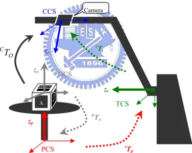
In this section, we will introduce how to apply the CPC model to estimate the transformation matrices among the coordinate systems defined on the motorized object rig. As shown in Fig. 5, we define three axes of three different reference frames on the rig. Let zrc, zrt and zrp detnoe the z-axes of the camera coordinate system (CCS), the tilt-axis coordinate system (TCS), and the pan-axis coordinate system (PCS), respectively.

For convenience, let the camera be the “end-effector” of the motorized object rig. Thus, we can obtain the corresponding robot pose with the method described in Section 2.1. In general, the orientations of the x- and the y-axes of the coordinate systems need not to be specified in formulating the kinematics of the motorized object rig. Therefore, the redundant parameter βi in

(3) can be set to zero, and the transformation matrix from object coordinate system (OCS) to camera coordinate system (CCS) can be simplified as follows:

2 2 1 1 0 0 V Q V Q V Q T T T T = × ×p _o= × × × × × p t t c o c (7) where bTa denotes the transformation matrix from coordinate system a to coordinate

system b.

Since the motorized object rig is composed of two revolution joints, the motion matrix Q0

is a constant matrix which can be set to identity, whereas Q1 and Q2 are the rotation matrices

about the zrt- and the zrp-axes, respectively. The equations of Q0, Q1 and Q2 are given by

p p p p z t t t t z q sign q sign ′ × = = ′ × = = = × φ φ θ θ where ), ( where ), ( 2 1 4 4 0 Rot Q Rot Q I Q (8) where signt and signp are either +1 or -1, and qt’ and qp’ are the rotation angle about the tilt and

14

[

] [

]

⎥ ⎦ ⎤ ⎢ ⎣ ⎡ = × × × × × × × = × × × × = × × × 1 ) , ( ) , ( ) ( ) ( ) ( ) ( ) ( ) ( ) ( 3 1 1 3 3 3 2 2 1 1 0 0 2 1 0 0 t r l Trans R Rot l Trans R Rot l Trans R Rot V Rot V T p t o c p t o c p z t z p z t z o c _V φ θ φ θ φ θ φ θ r (9)

where cro and cto are the rotation matrix and the translation vector of the transformation matrix c_T o. From (9), we have 2 1 0 ( ) ( ) ) , ( r r r r r r_{o t p} = × _{z t} × × _{z p} × c _{θ φ θ φ} (10) and

( )

1 1 0

( )

1

( )

2 2 0 0 0 c_tr_{( , )=r ×}r_{l +r ×r ×r×l}r_{+r ×r ×r ×r ×r ×l}r p z t z t z p t o θ φ θ θ φ (11)

In the following subsections, we will show how to solve the parameters, r0, l0 r , r1, l1 r , r2, l2 r in (10) and (11).

Fig. 5. The schematic of motorized object rig.

2.3.1. Rotation Parts 

In order to simplify the calibration process, we calibrate one axis at a time. Therefore, when calibrating the tilt-axis, the pan-axis is held still, i.e., φp can be regarded as a constant,

and thus r1×rz(φp)×r2becomes a constant term denoted by x. By substituting x into (10), we t_T p O C_T OCS CCS TCS zt p_T o PCS zp c_T t zc zo Camera A

15 have

( )

x r r r_{o t p} = × _{z j} × c _{θ φ θ} 0 ) , ( ₍₁₂₎

Equation (12) can be rewritten in the following form ) , ( ) ( 1 0 o i p c j z θ r r θ φ r x_{= −} − (13) By maneuver the tilt axis to two different joint values, θi and θj, from (12) and (13), we

have ) ( ) , ( ) , ( 1 _{0 0} j i z p j o c p i o c_{r θ φ × r θ φ} − _{×r =r ×r θ −θ (14)}

Multiplying [0 0 1]t on both sides of (14), we have

(

)

(

)

[

]

0 ) , ( ) , ( ) , ( ) , ( 0 0 3 3 3 3 1 0 0 1 ε ε φ θ φ θ φ θ φ θ = ⇒ ≈ = × − × ⇒ = × × × × − − b a b I r r b b r r r r r r p j o c p i o c p j o c p i o c (15)

where ε denotes the error vector induced by the observation noise, and b0 r

can be estimated by minimizing 2

ε . It is well known that b0 r

is the unit eigenvector of ata corresponding to the smallest eigenvalue λ. Note that the direction of b0

r

has to be determined such that its z-component is positive. By substituting the estimated b0

r

into (4), we have the orientation matrix R0.

The stability of the solution to b0 r

can be realized with the following derivation. By substituting (12) to the definition of a we have

1 0 0 3 3 ) ( -j i z a a r r r r I r a θ θ − = − = _× (16) From (16), it is obvious that b0

r

is the rotation axis of ra. However, if the difference of the

rotation angles (θi-θj) is close to zero, estimating the rotation axis of ra becomes ill-posed and

then the solution to b0 r

may not be stable. To avoid this singular configuration, one must make (θi-θj) as large as possible. This gives a useful guidance to selecting the joint angles for

kinematics calibration.

16

(

)

(

)

) ( ) , ( ) , ( 0 0 0 1 i t z j i z p j o c p i o c q sign ×Δ ′ × = − × = × × − r r r r r r r θ φ θ φ θ θ (17) The sign parameter signt can be determined by minimizing the following function

⎭ ⎬ ⎫ ⎩ ⎨ ⎧ × × − Δ × × = _∑ = − − + = M j o j p c p i o c i t z sign t sign q sign t 1 2 0 1 ' 0 1 , 1 ( ) ( , ) ( ( , )) min arg r r r θ φ r θ φ r ₍₁₈₎

Our next step is to solve the rotation matrix r1 of tTp also using (10). Now that r0 is

calibrated, the tilt axis can be moved when calibrating r1. For convenience, let us define

( )

(

)

( , ) ) , ( ~ 1 0 o t p c t z p t o c_{r θ φ = r ×r θ} −_{× r θ φ} (19) By maneuvering the pan axis to two joint angles, say φi and φj, from (10) and (19), we have

( )

( )

2 1 2 1 ) , ( ~ ) , ( ~ r r r r r r r r × × = × × = j z j j o c i z i i o c φ φ θ φ φ θ (20) Equation (20) can be rewritten as follows

( ) ( )

( )

( )

~( , ) ) , ( ~ 1 1 1 1 2 j j o c j z i i o c i z φ θ φ φ θ φ r r r r r r r × × − = × × − = − − (21) where yields

(

o j j

)

z

(

i j

)

c i i o c_{r θ φ × r θ φ} − _{×r =r ×r φ −φ} 1 1 1 ) , ( ~ ) , ( ~ ₍₂₂₎

Multiplying [0 0 1]t on both sides of (22), we have

(

)

(

)

[

]

ε ε φ θ φ θ φ θ φ θ = ⇒ ≈ = × − × ⇒ = × × × × − − 1 1 3 3 3 3 1 1 1 1 , 0 ) , ( ~ ) , ( ~ , ) , ( ~ ) , ( ~ b a b I r r b b r r r r r r j j o c i i o c j j o c i i o c (23)

Again, by solving an eigenvalue problem, we obtain b1 r

which leads to the rotation matrix r1.

The sign parameter signp for φp, and also be determined by minimizing an objective function similar to (18).

The final orientation parameter r2 can be computed with the following objective function

derived from (10). ∑ − × × × × j i o i j z i z j F c , 2 2 1 0 ( ) ( ) ) , ( min 2 r r r r r r r θ φ θ φ subject to r2r2 = I3×3 t _{and det 1} 2= r ₍₂₄₎

17

This constrained optimization problem can be solved with a method similar to the one proposed in [3].

2.3.2. Translation Parts 

By substituting the estimated rotation matrices into (11), we have the following linear equations for the translation parameters:

t z y x y x y x x o c _{[l l 0 l l 0 l l l ]} , 2 , 2 , 2 , 1 , 1 , 0 , 0 9 3 M t = r (25) where M3x9 =[r0 r0×rz(θ1)×r1 r0×rz(θ1)×r1×rz(φ1)×r2].

By moving the pan and the tilt joints to different positions, we have an over-determined system of the translation parameters which can be solved using the least square method.

2.3.3. Axes Adjustment 

After solving the kinematic parameters of the motorized object rig, we can compute its forward kinematic model as follows:

( )

( )

( )

( ) ) ( ) , ( 2 2 1 1 0 0 2 2 1 1 0 l Trans R Rot l Trans R Rot l Trans R V Q V Q V T r r r × × × × × × × = × × × × = p z t z p t o c φ θ φ θ (26) Given the tilt angle, θt, and the pan angle, φp, we can use (26) to determine the pose of the

camera. Also, the forward kinematic model can be used to find the representations of zrc, zrt and zrp axes, i.e., the orientation and position of these three axes. First, the transformation matrix from the reference frame of the tilt axis to the CCS can be determined as Tt =V0

c _{. Thus,}

the unit direction vector of the tilt axis zrt, denoted by Ot

r

, can be derived as follows

[

]

t

[

]

t

t c

t= T × 0 0 1 0 =V0× 0 0 1 0

Or (27)

The position of the tilt axis, denoted by Pt

r , is given by (28)

[

]

t

[

]

t t c t=T × 0 0 0 1 =V0× 0 0 0 1 Pr (28)

Similarly, the orientation and position of the pan axis zrp, denoted by Op r

and Pp r

18 found to be

[

]

[

]

t z t p t t c p= T×T 0 0 1 0 =V0×Rot ×V1× 0 0 1 0 Or (29) and

[

]

[

]

t z t p t t c p= T×T 0 0 0 1 =V0×Rot ×V1× 0 0 0 1 Pr , (30) respectively.

By using equations (27)-(30), the positions and orientations of the three axes of zrc, zrt and p

z

r _{can be evaluated and then can be illustrated as shown in Fig. 6(a). The positions of these} three axes can be adjusted to minimize the distance among them. According to our experiences, when the maximum distance among these three axes is smaller than a threshold value of 15 mm, the effect of the miss-alignment of these three axes is negligible.

2.4. Experimental Results of Calibration

Our method is implemented on the PC platform with CPU P4-3.0GHz and 1GB RAM and the motorized object rig is AutoQTVR. Fig. 6 shows the result before aligning the three axes of the rig where the estimates of the three axes are shown in Fig. 6(a), and the acquired OM of a toy shark is shown in Fig. 6 (b). The estimation and adjustment process is repeated five times to align the three axes of the rig and the result is shown in Fig. 7. From the frontal view of Fig. 7(d), we show that the tilt axis can be effectively adjusted to be perpendicular to the pan axis and optical axis of camera with our method. Moreover, from the top view of Fig. 7 (d), the intersections of the three axes are close enough. Some images of the OM of the toy shark are shown in Fig. 7(a). After the visual hull of the shark is constructed, shown in Fig. 7(c), the centralization process can be performed, and the resulted OM is shown in Fig. 7(b).

The process time (includes capturing time and computation time) of the calibration process relies on the amounts of the photographs are used. To reduce the process time we have to use small amounts of the photographs. Therefore, we generate some synthetic data to investigate

19

how many photographs we need and what the relations between the amounts of photographs and the accuracy of the estimated parameters are. We use 3D Studio Max to render the PCC object with known camera parameters. Three sets of synthetic data with different numbers of images (48, 24 and 12 images, respectively) are generated. The 48-image set is obtained with four different tilt angles (θt= 90°, 60°, 30°,and 0°) and twelve different pan angles (φp is from 0°

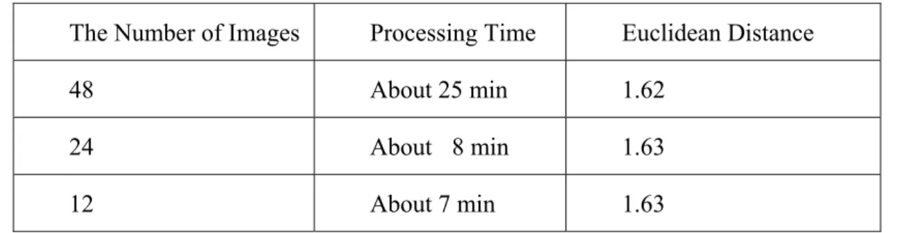
to 330° with an angle interval of 30 degree). The 24-image set is taken with three different tilt angles (90°, 60°, 30°) and eight different pan angles, and the 12-image set are taken with three different tilt angles (90°, 60°, 30°) and four different pan angles. In the experiments, our method is applied to the three data sets to estimate the camera parameters and the estimated parameters are compared with the ground truth. To quantify the error of the estimated camera parameters, some 3D points are randomly selected to calculate their 2D positions using the ground truth and the estimated camera parameters, and then the Euclidean distance between the ground-truth position and the estimated position is calculated. The results are shown in Table 1. The process time includes shooting process and camera parameter estimation. The error is mean Euclidean distance. From our experiments, we found that only 12 images are enough to obtain a set of highly accurate parameters. That is, we only need to take 12 pictures at each adjustment-calibration process, and the processing time needed, including capturing and processing, is about 7 minutes.

Table 1. Processing time and accuracy of the calibration processing

The Number of Images Processing Time Euclidean Distance

48 About 25 min 1.62

24 About 8 min 1.63

20 (a)

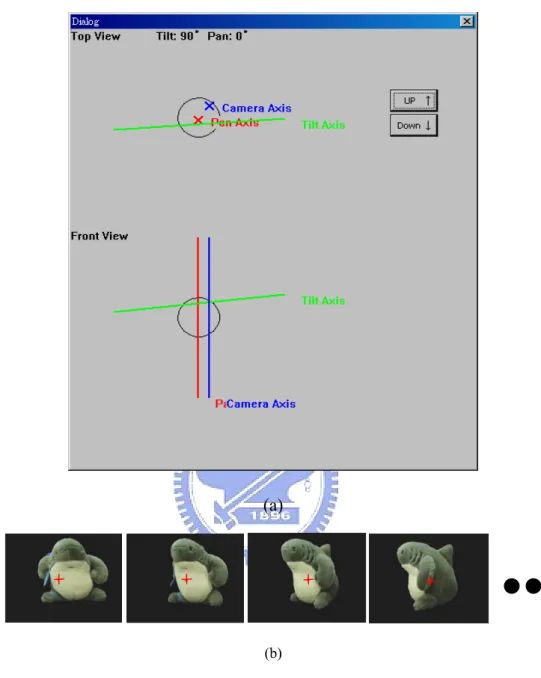
(b)

Fig. 6. The OM of the toy shark before calibration. (a) shows the estimated relation among 3 axes, and (b) shows the OM of the toy shark. The cross markers indicate the center of images.

21 (a)

(b)

(c)

(d)

Fig. 7. The result of the toy shark experient. (a) shows some images of the OM of the toy shark after calibration, while (b) shows that after centralization. (c) shows the Visual Hull of the shark, and (d) shows the estimated axes after calibration.

22

Chatper 3

Background Removal

In order to reduce the user intervention, the basic idea to develop the OM background removal system is follows. First, an automatic segmentation will be applied to obtain initial segmentation results. If some results are not satisfied, the user can correct one of them though the provided user interface. After modification, the corrected result can be automatically propagated to the other images, and used to refine the segmentation results.

In this work, we treat the segmentation problem as a labeling problem. We assign every pixel a label for a given OM. These labels are F (Foreground), B (Background), and U (Uncertain), and the image used to record the labels is called trimap. OM notations to which we will refer are: is defined as follows. Let Iθ ,φ denote the image taken at pan angle θ and tilt

angle φ. An equi-tilt set Oφ is defined as a subset of the images in an OM captured at the same

tilt angle φ, i.e.,

} 2 0 | { = θ,φ θ π φ I ≤ ≤ O ₍₃₁₎ Finally, an OM O is defined as } 2 2 , 2 0 | { } 2 2 | { = , π φ π π θ π φ π φ θ φ ≤ ≤ − ≤ ≤ = ≤ ≤ − I O O (32) Fig. 8 shows a portion of the two equi-tilt sets that are contained in the OM of the pottery owl.

Based on the idea, the flowchart of our system is shown in Fig. 9. It includes three main stages: initial labeling, label updating, and alpha estimation. For initial labeling, we extract reliable foreground and background pixels based on some OM characteristics. The details are described in section 3.1. For label updating, U pixels are updated using spatial and temporal coherence based on the extracted foreground and background. After label updating,

23

intermediate segmentation may contain some misclassified pixels. To correctly classify these pixels, user modification can be done at this point through the provided user interface. After modification, the label updating stage is again used to obtain more accurate results. After user intervention, most pixels are classified as foreground or background except the pixels that may be composites of the foreground and background. For alpha estimation, the method proposed by Chuang et al. [13] can be applied to calculate the alpha value for each U pixel. Using the alpha value, we can product a smooth contour blending when we integrate OM into a new background.

Fig. 8. Part of the two different equi-tilt sets before applying the OM segmentation method. Except for leftmost two images in the figure, the remainder of the images in this thesis are cropped in order to show more examples.

In this thesis, two approaches are proposed to propagate the corrected information. The first method utilizes motion vectors to propagate the corrected information to other frames that some segmentation errors occur. The details are described in section 3.2. The method works well for most cases, but requires more user intervention for some cases due to error motions.

The situation could be even worse for the first method. To compute the motion field, the motion estimator usually assumes that the sampling rate of the video camera is high enough to minimize the frame-to-frame motion. However, to keep the data size and cost reasonable, the

24

sampling rate of the OM is generally low. A popular alternative approach is to interpolate the dense motion field from a set of image correspondences. Because the difference between the images is caused fully by the changes in the 3D viewpoints, the perspective distortion makes the correspondence problem extremely difficult. In our experience, generating enough correspondences is still a problem, even with some popular tools, e.g., such as the KLT feature tracker [52] or the SIFT features [34]. Additionally, to filter out the potentially false correspondences, the class of the transformation, e.g., translational, affine, or a more complex -transformation, need to be considered so that the images can be aligned as accurately as possible, and a robust estimation can be performed. The translational motion is often the prominent transformation in many of the video source used to demonstrate the information propagation scheme. However, the nature of the transformation existed in the OM cannot be easily modeled without 3D object information. In practice, without some user intervention or knowledge of the 3D information, a usable motion field between any possible pair of the neighboring images in the OM is quite hard to compute. Therefore, the second approach is proposed for efficiently propagate the corrected information by learning shape priors. The details are described in section 3.3.

25

Fig. 9. The flowchart of segmentation method.

3.1. Initial Labeling

From our observation, OM has three basic characteristics which can help the method generate the trimap:

1. When an equi-tilt set of the OM is captured, a large proportion of the background

scene is static.

2. Only one interesting object is presented in every image of the OM.

3. The foreground and background color distributions are distinct in most cases.

The trimap labeling method comprises B-labeling and F-labeling. Each equi-tilt set of the OM is processed individually by the trimap labeling method. Given an equi-tilt set Oφ, the

26

trimap of each image in Oφ is initialized to U. During the B-labeling, pixels are examined to be

labeled as B based on the color difference. During the F-labeling, all pixels that are still labeled as U are examined to be labeled F based on the background model.

1.) B-labeling: By the first characteristic, if the color of a pixel varies barely throughout the

equi-tilt set Oφ, then the pixel should be the background and labeled B. Since an equi-tilt

set Oφ can be treated as a short video sequence, a pixel B is labeled by examining its color

difference compared with the corresponding pixels in both directions of the video sequence. Let p = [u v]T denote a pixel of a video frame It, i.e., an image of the equi-tilt set Oφ. Let It(p) be the color of pixel p in the frame It. Let Nt be the set of neighboring frames of It. To relieve the camera noises and consider the color changes caused by the lighting, a measure based on the block color difference with respect to the mean is used such that the background pixels can be recognized reliably. Each pixel p in It is labeled B if B N J tM p J ω < ∈ ∀min ( , ) (33)

Here, ωB is the threshold ensuring that only the pixel with a small color variation is labeled B. The measure M( Jp, ) is defined as follows

2 )) ( ) ( ( )) ( ) ( ( | | 1 ) , ( ∑ ∈ ∀ − − − = W x t t p J x J p I x I W J p M ₍₃₄₎

where W is a small window centered at the pixel p, | W| denotes the number of pixels in the window, It( p) is the mean color of the window W on the image It. J( p) is the mean color of the window W on the image J, and |•|2 denotes the L2-norm. For each pixel on a

frame It, the measure is examined in both directions of the video sequence, i.e., backward and forward. Figure 4 shows a portion of the equi-tilt set after applying the above procedure, where Nt ={It−1,It+1}.

Most of the B pixels are exactly within the background as shown in Fig. 10, but there are exceptions, such as the pixels of a uniform colored patch of the object. The concept of

27

label consistency is then introduced. If the pixels at the same image position do not have the same label throughout the whole sequence, then they are re-labeled as U. Finally, by the second characteristic of the OM, mathematical morphology is applied to filter out the remained noises such that only one U region exists, surrounded by the B region. Notably, all the images in Oφ until now had the same trimap consisting only the B and U labels. Fig.

11 shows an example of such a global background mask.

Fig. 10 The top row shows a portion of the input image sequence taken from an equi-tilt set of the pottery owl OM. For all the images in the middle and bottom rows, the black pixels correspond to the classified background regions. The foreground regions are colored white, and the unknown regions are colored gray. The middle row shows the corresponding result during the B-labeling for each image. Notably, to filter out the incorrectly classified pixels and obtain the global background mask used during F-labeling, label consistency and mathematical morphology are used as shown in Fig. 11. Finally, the bottom rows shows the generated trimap for each image that is used to activate the graph cut image segmentation.

2.) F-labeling: By the third characteristic of the OM, each pixel whose color differs widely

from the background model can be labeled F. To learn the background model of a given image, the B pixels that are reasonably close to the boundary between the B and U regions

28

are collected and clustered by using K-means. Let i φ θ

μ _, denote the mean color of the ith cluster for image Iθ ,φ. Each pixel p with the label U in the image Iθ ,φ is examined and

labeled F if F i i Iθφ p −μθφ <ω ∀ , ( ) , 2 min ₍₃₅₎

where ωF is a strict threshold to ensure that only the pixels that differ widely from the background model are labeled F.

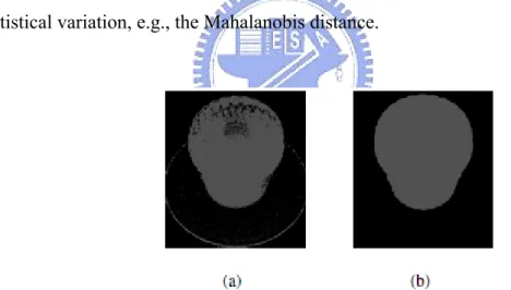
Fig. 10 shows the result of the trimap labeling. The trimap of each image is used to activate the graph cut image segmentation. Notably, in this OM segmentation problem, the variation between the colors drawn from the background and foreground is strong. Thus, for a given pixel, to determine the similarity of its color to the foreground or background model in the graph cut image segmentation, the distance measure should consider the statistical variation, e.g., the Mahalanobis distance.

Fig. 11. (a) The result including the label consistency concept is included; (b) The global background mask obtained by applying the mathematical morphology on (a).

3.2. Label Updating with Motion Vectors

The label updating stage consists of spatial (intra-frame) updating and temporal (inter-frame) updating. The spatial followed by the temporal updating process will be iterated until it is stable. That is, label updating will repeat until there is no label change.