A Hybrid Data Mining Architecture for Customer Retention

全文

(1)2002 International Computer Symposium (ICS2002) Name of the workshop: Workshop on Artificial Intelligence Title: A Hybrid Data Mining Architecture for Customer Retention Abstract: Competition in the wireless telecommunications industry is fierce. To maintain profitability, wireless carriers must control churn, which is the loss of subscribers who switch from one carrier to another. This paper proposes a hybrid architecture that tackles the complete customer retention problem, in the sense that it not only predicts churn probability but also proposes retention policies. The architecture works in two modes, namely, the learning and usage modes. In the learning mode, it learns potential associations inside the historical subscriber database to form a churn model. It then uses the attributes that appear in the churn model to segment all churners into distinct groups. It is also responsible for developing a specific policy model for each churner group. In the usage mode, the churner predictor uses the churn model to predict the churn probability of a given subscriber. A high churn probability will cause the system suggest specific retention policies according to the policy model. Our experiments illustrate that the churn prediction has around 85% of correctness in evaluation. Currently, we have no proper data to evaluate the constructed policy model. The policy construction process, however, signifies an interesting and important approach toward a better support in retaining possible churners. Author: Ming - Shian Tsai 1 , Bong - Horng Chu 2 , Cheng - Seen Ho 3 Current affiliation: Department of Electronic Engineering, National Taiwan University of Science and Technology Postal address: 43, Sec. 4, Keelung Rd., Taipei, TAIWAN, 106 E-mail:. 1. cobila@ailab2.et.ntust.edu.tw, 2 ben@ailab2.et.ntust.edu.tw, 3 csho@et.ntust.edu.tw. Telephone: (02) 27336381 Contact author: Cheng-Seen Ho Keywords: Churn, Classification, Clustering, Customer retention, Data mining, Decision tree, SOM.. 1.

(2) A Hybrid Data Mining Architecture for Customer Retention Ming - Shian Tsai 1. Bong - Horng Chu 2. Cheng - Seen Ho 3. Department of Electronic Engineering National Taiwan University of Science and Technology. 43, Sec. 4, Keelung Rd., Taipei, TAIWAN, 106 E-mail:. 1. cobila@ailab2.et.ntust.edu.tw, 2ben@ailab2.et.ntust.edu.tw, 3csho@et.ntust.edu.tw. Abstract. Competition in the wireless telecommunications industry is fierce. To maintain profitability, wireless carriers must control churn, which is the loss of subscribers who switch from one carrier to another. This paper proposes a hybrid architecture that tackles the complete customer retention problem, in the sense that it not only predicts churn probability but also proposes retention policies. The architecture works in two modes, namely, the learning and usage modes. In the learning mode, it learns potential associations inside the historical subscriber database to form a churn model. It then uses the attributes that appear in the churn model to segment all churners into distinct groups. It is also responsible for developing a specific policy model for each churner group. In the usage mode, the churner predictor uses the churn model to predict the churn probability of a given subscriber. A high churn probability will cause the system suggest specific retention policies according to the policy model. Our experiments illustrate that the churn prediction has around 85% of correctness in evaluation. Currently, we have no proper data to evaluate the constructed policy model. The policy construction process, however, signifies an interesting and important approach toward a better support in retaining possible churners.. Keywords: Churn, Classification, Clustering, Customer retention, Data mining, Decision tree, SOM. 2.

(3) 1. Introduction. Customer Relationship Management (CRM) has made a high profile entry into business over the past few years. Although it’s been around for many years in the form of customer service, advances in technology and increased competition have driven companies to improve customer satisfaction and loyalty to maintain healthy profits. A 5% increase in customer retention results in as much as a 75% increase in profitability [INDI2002]. CRM is particularly important in the industry of wireless telecommunications, since the competition in the wireless telecommunications industry is fierce. The industry is extremely dynamic, with new services, technologies, and carriers coming up so often. Carriers announce new rates and incentives weekly, hoping to entice new subscribers and to keep subscribers away from the competitors. The extent of this rivalry is reflected in the inundated advertisements for wireless service in daily newspapers and related mass media [Moze2000].. Growing competition, however, has forced companies to invest significant resources in attaining new customers. Unfortunately, a typical service provider loses four percent or more of its subscribers each month due to sheer competition, which translates to millions of dollars of revenue both today and in the future [Howl2000]. Given the relatively high cost of covering these losses by acquiring new subscribers, companies have become increasingly focused on retaining their customers.. 3.

(4) Customer churning, customers switching from one carrier to another, can dramatically destroy the profits of the carriers and has become a major issue in CRM. It is often stated that the cost of acquiring a new customer is 5 to 10 times greater than that of retaining existing ones. Churning costs wireless carriers a total of more than $4 billion each year [Ande2000]. It is thus justified to find better means of ensuring that the subscribers remain loyal. In other words, it is crucial to predict subscribers’ behavior. Accurate prediction may allow carriers to forestall churning by proactively building lasting relationships with subscribers. This is especially true for telecommunications when considering the most profitable subscribers, as it is commonly accepted that 20% of the subscribers are responsible for generating 80% of the profit. Therefore it is important to realize that when attrition will doubtless occur, the carriers should start targeting their preventive strategies at those subscribers who contribute most to the carriers, which might include increasing the level of service available to the subscribers. For those subscribers who are likely to churn, the carriers can embark on a policy of trying to catch them back. In general, the carriers should take proactive steps to keep valuable subscribers from defecting, thereby, keeping subscribers loyal and satisfied in order to increase the profits. Some carriers have begun to look at their churn data, typically examining a small number of variables and searching for their dependencies using traditional statistical models [Gerp2001]. Some even go one step further by employing data mining techniques hoping to obtain better results.. Many researches have started to establish what enables a company to retain its subscribers in the long run. A large amount of investigations have been undertaken on the topic of customer 4.

(5) retention[Moze2000] [Yan2001] [SAS2001]. These previous investigations did highlight the impact of many situations on customer retention. However, almost all studies were focusing on increasing the accuracy of predicting churn without touching the issue of making appropriate policies according to the analysis of the churn problem. The problem is that we can’t reduce the churn rate simply by predicting churn without forestalling it. We need more analysis.. In general, churn can be the result of a number of factors. Price typically drives churn as subscribers seek for lower rates on service agreements. While competitive pricing is a major reason for churn, factors such as customer service, service quality and regional coverage also cause customer defection. This further strengthens the idea that we can’t just predict churn; we have to find out the reasons why the subscribers defect, and make proper policies accordingly to retain them. Only after this can we say that we have completely dealt with customer retention. In other words, we should search for an approach for customer retention that not only predicts churning but also makes proper policies to forestall it.. In this paper, we propose a hybrid architecture to completely take care of the customer retention problem. The architecture works in two modes, i.e. learning and usage modes. In the learning mode, it constructs a churn model that can analyze and predict the probability of churning. It also constructs a policy model that clusters the churners by labeling each cluster with most significant attributes, and accordingly creates specific proper policies for each cluster. During the usage mode, the churn model. 5.

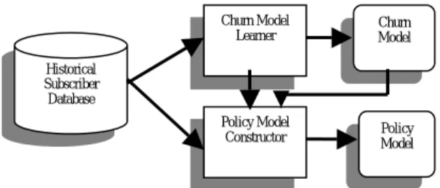
(6) is used to determine whether a given customer is going to defect. If so, the policy model is used to propose a specific policy to retain the customer. The most significant feature of the approach is that it not only predicts churn but also forestalls churn.. 2. System Architecture. Our hybrid customer retention system runs in two modes: the learning and usage modes. Fig. 1 shows the architecture in the learning mode. In this mode, we are working on constructing a churn model and a policy model. The former uses the classification technique to learn under what conditions a subscriber may churn. The latter analyzes the churn model using the clustering technique and develops how policies can be associated with the clustered churners. The classification technique is based on C5.0 [Quin1993], while the clustering technique is based on an improved version of GHSOM [Ditt2000]. We abstract the basic ideas of these two techniques in Appendix A and B, respectively.. Churn Model Learner. Churn Model. Policy Model Constructor. Policy Model. Historical Subscriber Database. Fig. 1 System architecture in learning mode. Once the models are developed and tested, the system can be put in the usage mode. Fig. 2 shows the architecture in this mode. Now given a subscriber, the system can use the churn model to predict. 6.

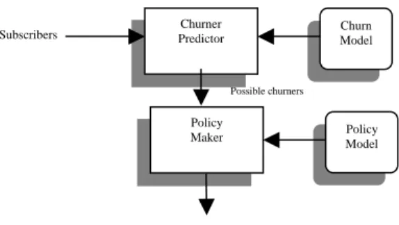
(7) whether he is going to churn. If yes, the policy model is then used to further analyze his data and propose a proper policy to retain the customer.. Subscribers. Churner Predictor. Churn Model. Possible churners. Policy Maker. Policy Model. Retention Policies. Fig. 2 System architecture in usage mode. The following subsections detail each component in the learning mode and show how the usage mode is working.. 2.1 Churn Model Learner. This module learns the churn model using C5.0. The input is the historical subscriber database, which contains historical details of each individual subscriber, including defection history, de-activation data, payment histories, usage patterns, trends and changes. Out of its hundreds of attributes we have identified 12 variables we conjectured are most likely to be linked to churn, as shown in Table 1.. 7.

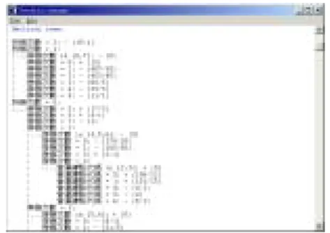
(8) Table 1 The attributes conjectured to be relevant to churn Attribute Gender (性別). Content 0 for male, 1 for company, and 2 for female 0 for Public, 1 for Business, 2 for Manufacture, 3 for Finance, 4 for. Industry code (客戶業別). Communication, 5 for DepartmentStore, 6 for SocialService, 7 for Farming and Ffor hing, 8 for individual, and 9 for Other. Dealer ID (通路代碼) Site (營運據點代碼). 0~10 0 for Site1, 1 for Site2, 2 for Site3, 3 for Site4, 4 for Site5, 5 for Site6, and 6 for Site7 0 for Standard, 1 for Economy, 2 for Prepay, 3 for Ultra Low Rate, 4 for. Package code (申租費率). Base Rate, 5 for Base Rate plus 100, 6 for Base Rate plus 400, 7 for Base Rate plus 800, 8 for Base Rate plus 1500, and 9 for Special Low Rate 0 for Government, 1 for GuarantyFree, 2 for PrepaidCard, 3 for Normal,. Discount type (優惠類別). 4 for Enterprise, 5 for Employee, 6 for Military, 7 for Offical, 8 for PublicServant, 9 for Alliance, and 10 for Subordinate. Tenure (租期). 0 for 0~4, 1 for 5~13, 2 for 14~25, 3 26~37, 4 for 38~61, and 5 for over 62. Stop-use (停機次數). 0~9. Re-use (復機次數). 0~7. Disconnect (拆機次數). 0~2. Average Invoice (平均費用). 0 for 0~100, 1 for 101~200, 2 for 201~500, 3 for 501~1000, 4 for 1001~2000, 5 for 2001~3000, and 6 for over 3001. The churn model learned by the module is represented by a decision tree as illustrated in Fig. 3. Each leaf is followed by a parenthesis (N/E), which means out of N cases in this leaf, E cases are misclassified. Note that each path in the decision tree is a rule.. Fig. 3 A snapshot of part of churn model 8.

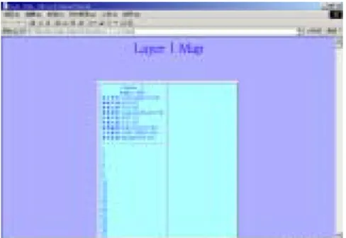
(9) 2.2 Policy Model Constructor. This module constructs interaction strategies: what incentives should be offered to which kinds of churners. This involves two tasks. First we need to dig out the implicit relationships between churners. Basically, we use a “modified GHSOM” to discover the clusters inside the churners. Then, we need to propose specific policies for each cluster of churners according to the interpretation of the cluster.. Specially, we consult the learned churn model and collect all the attributes that are recognized by the model as having strong relations with churning. Then we feed all the churners data, in terms of the above attributes, to the modified GHSOM, which then segments all churners into different clusters and labels the most common attributes in each cluster, as shown in Fig. 4.. Fig. 4 Example of a GHSOM segmented cluster. Note that we mentioned “modified GHSOM”. This is because there is an obvious shortcoming about GHSOM. That is, GHSOM can not deal with unknown attribute values. The real world data, however, often contain lots of missing attribute values. To cope with this, we introduce into GHSOM a probabilistic approach similar to C5.0. Formally, let T be a training set of cases. Assume a case from T. 9.

(10) contains attribute A which contains no values for a test X. Then we assign the test the following value.. n. ∑. Vi * P (Vi ) ,. i =0. where P( Vi ) is defined to be the ratio of the number of cases in T known to have value Vi over that in T with known values on this test.. To facilitate the analysis of each cluster, we have made a second improvement on GHSOM. Instead of just labeling important attributes in each cluster, we associate with them their most converging values. In addition, we associate each of the attribute-value pair with a percentage that calculates the frequency of the cases that contain the attribute value in each cluster. Furthermore, we rank these attributes in order of the percentage to show how converging the cases are for each attribute in the cluster. All these changes have been reflected in Fig. 4.. Finally, we analyze the attributes in each cluster, which logically represents a churner group, trying to give it an interpretation. Based on the interpretation, we then propose a set of proper policies suitable for retaining the subscribers. Fig. 5 illustrates the proposed policy model for the churner group of Fig. 4.. Cluster Cluster 1. Policy Policy 1: Suggest the subscribers to change to a more matchable basic monthly fee. Policy 2: Suggest the subscribers to prepay NT 1200 for deduction of NT 1400 from their monthly communication fees.. Fig. 5 Policy model for the churner group in Fig. 4. 10.

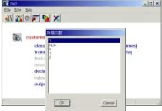
(11) 2.3 Usage Mode. In the usage mode, the churn predictor prompts proper dialog windows to solicit the subscriber data from the user, as shown in Fig. 6. It then uses the churn model to predict how likely he is going to churn. Fig. 7 shows that this specific subscriber has 0.67 probability to defect.. Fig. 6 Enter subscriber data to the churner predictor. Fig. 7 Churn probability predicted by the churner predictor. Since this subscriber is likely to churn, with probability above 60%, the policy maker is invoked to determine which cluster, i.e., churner group, he may belong to and utilize the policy model to propose some proper policies, as shown in Fig. 8.. 11.

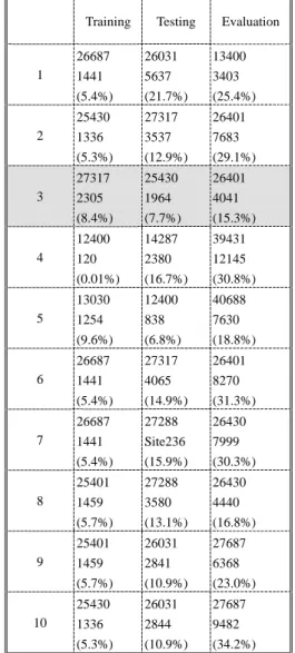
(12) Fig. 8 Proposed policies by the policy maker. 3. Experimental Results. The system is implemented using Borland C++ Builder 5.0 and Visual C++ 6.0. The subscriber database used for our experiments was provided by a major wireless carrier in Taiwan. The database consists of 65516 business subscribers. The subscribers come from all regions of Taiwan during the time interval of July 2001. Based on the carrier’s definition of churn, which means the closing of all services held by a subscriber, 15600 of the subscribers active in July churned, about 23.8% of the whole database.. In order to get around any possible bias of a real world database, we divided the whole database into 5 partitions, and randomly selected and/or combined different partitions for training, testing, and evaluation. Table 2 illustrates 10 of the experimental results. In each cell of the table, item 1 is the number of cases, item 2 is the number of errors, and item 3 in the parenthesis is the error rate. Combination 3 in the table is selected to produce churn model due to its comparatively stable and less error rates.. 12.

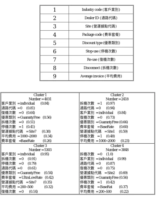
(13) Table 2 Results of different combinations of database partitions Training. 1. 2. 3. 4. 5. 6. 7. 8. 9. 10. Testing. Evaluation. 26687. 26031. 13400. 1441. 5637. 3403. (5.4%). (21.7%). (25.4%). 25430. 27317. 26401. 1336. 3537. 7683. (5.3%). (12.9%). (29.1%). 27317. 25430. 26401. 2305. 1964. 4041. (8.4%). (7.7%). (15.3%). 12400. 14287. 39431. 120. 2380. 12145. (0.01%). (16.7%). (30.8%). 13030. 12400. 40688. 1254. 838. 7630. (9.6%). (6.8%). (18.8%). 26687. 27317. 26401. 1441. 4065. 8270. (5.4%). (14.9%). (31.3%). 26687. 27288. 26430. 1441. Site236. 7999. (5.4%). (15.9%). (30.3%). 25401. 27288. 26430. 1459. 3580. 4440. (5.7%). (13.1%). (16.8%). 25401. 26031. 27687. 1459. 2841. 6368. (5.7%). (10.9%). (23.0%). 25430. 26031. 27687. 1336. 2844. 9482. (5.3%). (10.9%). (34.2%). We found only nine attributes appear in the churn model as listed in Table 3. We thus feed all the 15600 cases in terms of the nine attributes into the modified GHSOM. Fig. 9 illustrates the results. There are 4 clusters; item 2 in each cluster stands for the number of subscribers in the cluster. From item 3 down to item 11 are the ranked important attributes according to their frequencies.. 13.

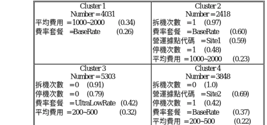
(14) Table 3 Attributes appearing in the churn model. 1. Industry code (客戶業別). 2. Dealer ID (通路代碼). 3. Site (營運據點代碼). 4. Package code (費率套餐). 5. Discount type (優惠類別). 6. Stop-use (停機次數). 7. Re-use (復機次數). 8. Disconnect (拆機次數). 9. Average invoice (平均費用). Cluster 1 Number = 4031 客戶業別 = individual (0.84) 通路代碼 = 0 (0.81) 復機次數 = 0 (0.64) 優惠類別 = GuarantyFree (0.56) 拆機次數 = 0 (0.51) 停機次數 = 1 (0.41) 營運據點代碼 = Site7 (0.38) 平均費用 = 1000~2000 (0.34) 費率套餐 =BaseRate (0.26) Cluster 3 Number = 5303 客戶業別 = individual (0.95) 拆機次數 = 0 (0.91) 停機次數 = 0 (0.79) 通路代碼 = 0 (0.61) 優惠類別 = GuarantyFree (0.54) 費率套餐 = UltraLowRate (0.42) 營運據點代碼 = Site7 (0.35) 平均費用 = 200~500 (0.32) 復機次數 = 0 (0.14). Cluster 2 Number = 2418 拆機次數 = 1 (0.97) 通路代碼 = 0 (0.94) 客戶業別 = individual (0.84) 復機次數 = 0 (0.73) 優惠類別 = GuarantyFree (0.66) 費率套餐 = BaseRate (0.60) 營運據點代碼 = Site1 (0.59) 停機次數 = 1 (0.48) 平均費用 = 1000~2000 (0.23) Cluster 4 Number = 3848 拆機次數 = 0 (1.0) 客戶業別 = individual (0.99) 通路代碼 = 0 (0.87) 復機次數 = 0 (0.75) 營運據點代碼 = Site2 (0.69) 優惠類別 = GuarantyFree (0.56) 停機次數 = 1 (0.42) 費率套餐 = BaseRat (0.37) 平均費用 = 200~500 (0.22). Fig. 9 Preliminary churner groups by GHSOM using attributes in the churn model. In order to distinguish the 4 clusters so that a specific meaningful interpretation can be given for each cluster, we first eliminate those attributes that appear in all clusters and contain the same values. They can be dealt with using some common policies. After further housekeeping on each cluster, we transform Fig. 9 into Fig. 10, which only lists the outstanding attributes in each group of churners. Now we can propose proper specific policies for each of the groups. Table 4 shows the policy model. 14.

(15) corresponding to each churner group. Cluster 1 Number = 4031 平均費用 = 1000~2000 (0.34) 費率套餐 =BaseRate (0.26). .. 拆機次數停機次數費率套餐平均費用. Cluster 3 Number = 5303 = 0 (0.91) = 0 (0.79) = UltraLowRate (0.42) = 200~500 (0.32). Cluster 2 Number = 2418 拆機次數 = 1 (0.97) 費率套餐 = BaseRate (0.60) 營運據點代碼 = Site1 (0.59) 停機次數 = 1 (0.48) 平均費用 = 1000~2000 (0.23) Cluster 4 Number = 3848 拆機次數 = 0 (1.0) 營運據點代碼 = Site2 (0.69) 停機次數 = 1 (0.42) 費率套餐 = BaseRate (0.37) 平均費用 = 200~500 (0.22). Fig. 10 Churner groups Table 4 Policy model (only specific policies shown) Cluster Cluster 1. Cluster 2. Cluster 3 Cluster 4. Policy Policy 1: Suggest the subscribers to change to a more matchable basic monthly fee. Policy 2: Suggest the subscribers to prepay NT 1200 for deduction of NT 1400 from their monthly communication fees. Policy 1: Delay one week before disconnection. Policy 2: Suggest the subscribers to change to a more matchable basic monthly fee. Policy 3: Improve the service attitude of a specific service center, e.g., site1. Policy 1: Reduce the communication fees of the subscribers by giving some discount. Policy 2: Encourage the subscribers to prepay NT 1200 for deduction of NT 1400 in the future 3 or 6 months. Policy 1: Make an attentive phone call to offer nice and warm regards. Policy 2: Check their complaint records in order to discover why they churn.. Let’s exemplify cluster 1 for explanation. For details see [Tsai2002]. In Cluster 1, we noticed that the invoices of these subscribers are much higher than their basic monthly fees. With a lower basic monthly fee, the charge on per-second communication tends to be higher. The subscribers in this cluster seem unaware that their communication time is well longer than what the basic monthly fee can provide and have been charged unfairly. If they somehow notice that, they surely churn. We thus suggest the following two policies:. Policy 1: Suggest the subscribers to change to a more matchable basic monthly fee. Policy 2: Suggest the subscribers to prepay NT 1200 for deduction of NT 1400 from their monthly communication fees.. 15.

(16) 5. Conclusions. We have described a hybrid architecture that tackles the complete customer retention problem, in the sense that it not only predicts churn probability but also proposes retention policies. The architecture works in two modes, namely, the learning and usage modes. In the learning mode, the churn model learner learns potential associations inside the historical subscriber database to form a churn model. The policy model constructor then uses the attributes that appear in the churn model to segment all churners into distinct groups. It is also responsible for developing a specific policy model for each churner group. In the usage mode, the churner predictor uses the churn model to predict the churn probability of a given subscriber. A high churn probability will cause the churner predictor to invoke the policy maker to suggest specific retention policies according to the policy model. Our experiments show that the learned churner model has around 85% of correctness in evaluation. Currently, we have no proper data to evaluate the constructed policy model. The construction process, however, signifies an interesting and important approach toward a better support in retaining possible churners.. This work is significant since the state-of-the-art technology only focuses on how to increase the accuracy of churn prediction. They either never touched the issue of retention policies, or only proposed policies according to the path conditions of the decision tree, the churn model. Our policy model construction process goes on step further to investigate the concept of churner groups, which equivalently digs out the associations between the paths of the decision tree. We believe with this 16.

(17) in-depth knowledge about how churns are related, we can propose better retention policy models for possible churners.. From the viewpoint of technology used in the system, our classification-followed-by-clustering approach. to. do. customer. retention. is. rather. unique. compared. with. the. common. clustering-followed-by-classification approaches [Boun2001]. It appears that our approach works well while we are dealing with making policies related to some known categories.. References [Ande2000] Anderson Consulting, “Battling Churn to Increase Shareholder Value: Wireless Challenge for the Future”, Anderson Consulting Research Report, 2000. [Boun2001] C. Bounsaythip and E. R. Runsala, “Overview of Data Mining for Customer Behavior Modeling”, VTT Information Technology research report, June 2001. [Cest1987] B. Cestnik, I. Kononenko, and I. Bratko, “ASSISTANT 86: A Knowledge-Elicitation Tool for Sophisticated Users”, Proceedings of Progress in Machine Learning, pp. 31-45, 1987.. [Ditt2000] M. Dittenbach, D. Merkl, and A. Rauber, “The Growing Hierarchical Self-Organizing Map”, Proceedings of the International Joint Conference on Neural Networks (IJCNN 2000), pp. 15-19, July 2000. [Gerp2001] T. J. Gerpott, W. Rams, and A. Schindler, “Customer Retention, Loyalty, and Satisfaction in the German Mobile Cellular Telecommunications Market”, Telecommunications Policy, Vol. 25, pp. 249-269, 2001.. [Howl2000] D. Howlett, “That Crazy Little Thing Called Churn”, Boardwatch Magazine, Vol. 3, pp. 23-45, April 2000. [Koho1982]. T. Kohonen, “Self-organized Formation of Topologically Correct Feature Maps”,. Biological Cybernetics, Vol. 43, No. 62,pp. 59-69, 1982. 17.

(18) [INDI2002] INDIGOlighthouse company, “Customer Relationship Management”, Available at http://www.indigolighthouse.com/crm.htm, 2002. [Modi1999] L. Modisette, “Milking Wireless Churn for Profit”, Telecommunications Online, Web page: http://www.telecoms-mag.com/default.asp, February 1999. [Moze2000] M. C. Mozer, R. Wolniewicz, and D. B. Grimes, “Predicting Subscriber Dissatisfaction and Improving Retention in the Wireless Telecommunications Industry”, IEEE Transactions on Neural Networks, Vol. 11, No. 3, pp. 690-696, MAY 2000. [Quin1983] J. R. Quinlan, “Induction of Decision Tree”, Machine Learning, Vol.1, pp. 81-106, 1983. [Quin1993] J. R. Quinlan, C4.5: Programs for Machine Learning, Morgan Kaufmann, San Mateo CA, 1993.. [SAS2001] SAS Company, “Predicting Churn: Analytical Strategies for Retaining Profitable Customers in the Telecommunications Industry”, A SAS White Paper, 2001. [Schm1999]. J. Schmitt, “Churn: Can Carriers Cope?”, Telecommunication Online, Web page:. http://www.telecoms-mag.com/default.asp, February 1999.. [Schw2001] E. Schweighofer, A. Rauber, and M. Dittenbach, “Automatic Text Representation, Classification and Labeling in European Law”, Proceedings of the 8th International Conference on Artificial Intelligence and Law (ICAIL 2001), pp. 21-25, May 2001. [Tsai2002] M.S. Tsai, A Hybrid Data Mining Model for Customer Retention, Master Thesis, National Taiwan University of Science and Technology, Taipei, Taiwan, 2002.. [Yan2001] L. Yan, D. J. Miller, M. C. Mozer, and R. Wolniewicz, “Improving Prediction of Customer Behavior in Nonstationary Environments”, Proceedings of International Joint Conference on Neural Network, Vol. 3, pp. 2258-2263, 2001.. 18.

(19) Appendix A Basics of C5.0. C5.0 is a well-known decision tree algorithm developed by Quinlan [Quin1993]. It introduces a number of extensions to the classical ID3 algorithm [Quin1983]. First, the selection of a test in ID3 was on the basis of the absolute gain criterion. In C5.0 the bias inherent in the gain criterion is rectified by some sort of normalization, which considers the entropy of a case to include not only which class the case belongs to, but also the outcome of the test. Suppose we have a possible test X on some attribute with n outcomes that partitions the set T of training cases into subsets T1 , T2 ....Tn . Formally, we define.  | T | | Ti | × log 2  i  i =1 | T |  |T | n. split _ entropy( X ) = − ∑. to be the potential information generated by partitioning T into n subsets. Now we can define a gain_ratio as the new metric measuring the information gain relevant to classification that arises from the same division. In other words,. gain _ ratio( X ) =. gain ( X ) split _ entropy ( X ). expresses the proportion of entropy normalized by the splits. Generally speaking, the gain ratio criterion is robust and can consistently give a better choice of tests than the gain criterion.. Second, in C5.0, continuous attributes are properly taken care of. First all the training cases in T are sorted on the values of a continuous attribute, say A. We denote them in order as {v1 , v2 , K , v m }. 19.

(20) Any threshold value between vi and vi +1 will have the same effect of dividing the cases into those whose value of the attribute A lies in {v1 ,v 2 ,K ,vi } and those whose value is in {vi +1 , vi + 2 ,K , vm }.. Finally, the basic algorithm to construct decision trees contains a hidden assumption that the outcome of a test for any case must be determined. But it is an unfortunate fact that data often has missing attribute values. Several algorithms have developed different answers to these problems, C5.0 adopts the probability approach. Let T be a training set and X be a test on some attribute A, and suppose that the value of A is known in fraction F of the cases in T. Let entropy (T ) and. entropy x (T ) be calculated as before, except that only the cases with known values of A are taken into account. The definition of gain can reasonably be modified to. gain ( X ) = probability A is known x ( entropy (T ) - entropy x (T ) ) + probability A is not known x 0 = F × ( entropy (T ) - entropy x (T ) ). Appendix B. Basics of GHSOM (The Growing Hierarchical Self-Organizing Map). The key point of GHSOM is to use a hierarchical neural network structure composed of a number of individual layers and each of them consists of independent SOMs [Raub2001]. The first step of the growth process measures the overall deviation of the input data against the single unit SOM at layer 0, which is assigned a weight vector m0 , the average of all input data. Formally, given d inputs. 20.

(21) [. [. ]. xi = µi1 , µi2 , µi3 ,K , µin , i = 1, 2, ….,d, we define m0 = µ01 , µ02 ,K , µ0n. where µ0i =. µ1i + µ 2i + L + µ di d. ]. T. ,. . The deviation of the input data, i.e., the mean quantization error of. this single unit, is computed below.. mqe0 =. 1 d × ∑ m0 − xi d i =1. We will refer to the mean quantization error of a unit as mqe in lower case letters.. The layer 1 initially consists of a rather few number of units, e.g. a grid of 2 × 2 units. Each of these units i is assigned an n-dimensional weight vector mi , defined by. [. ]. mi = µ i1 , µ i2 ,K , µ in , mi ∈ R n , T. and it is initialized with random values. It is important to note that the weight vectors must have the same dimensionality as the input patterns. The learning process of GHSOM is like a competition among the units to represent the input patterns [Schw2001].. In order to modify the size of each SOM, the mean quantization error of the map is computed as follows, where u is the number of units i contained in the SOM m.. MQE m =. 1 × ∑ mqei u i. The basic idea of growing is that each layer of the GHSOM is responsible for explaining some portion of the deviation of the input data as present in its preceding layer. This portion can be reduced. 21.

(22) by adding units to the SOM on each layer until a suitable size of the map is reached. More precisely, the SOM on each layer is allowed to grow until the deviation present in the unit of its preceding layer is reduced to at least a fixed parameter Tm . Obviously, the smaller the parameter Tm is chosen, the larger the size of the emerging SOM is. Formally, when the formula as follows is true for the map m,. MQE m ≥ Tm × mqei ,. there is either a new row or a new column of units needed to be added to this SOM. At first we must find the unit e with the greatest mean quantization error mqee , and let this unit be the error unit. The determination of whether a new row or a new column is inserted depends on the position of the most dissimilar neighboring unit to the error unit. The initial weight vectors of the new units are simply assigned as the average of the weight vectors of the existing neighbors. After the insertion, the learning rate parameter α and the neighborhood function hci are reset to their initial values and the training continues according to the standard training process of SOM.. 22.

(23)