A GA embedded dynamic search algorithm over a Petri net model for an FMS scheduling

(1)

Proceedings of the 1997

Intemattional Conference on Robotics and Automation Albuquerque, New Mexico

-

April 1997

A

GA

Embedded Dynamiic Search Algorithm over a Petri

Net Model

for an FMS Scheduling

Yung- Feng Chiu

La-Chen

Fu

Department

of

Computer Science and Information Engineering

National Taiwan University, Taipei, Taiwan, R.O.C.

January 27, 1997

Abstract

I n this paper, a genetic algorithm (GA) embedded dynamic search strategy over a Petri net model pro- vides a new scheduling method f o r a flexible manu- facturing system (FMS). The chromosome repnesen- tation of the search nodes is constructed directly from the Petri net model of an FMS, recording the infor- mation about all conflict resolutions, such as resource assignments and orders for resource allocation. The

GA operators may enforce some change to the chro-

mosome information an next generation. A Petri net based schedule builder receives a chromosome and a n initial marking as input, and then produces a near- optimal schedule.

Due to the NP-complete nature of the schedul- ing problem of a n FMS, we also propose a dynamic F M S scheduler incorporating the proposed GA embed- ded search scheme, which generates successive partial schedule, instead of generating a full schedule f o r all raw parts, as the production evolves.

1 Introduction

In FMS’s, generating a schedule to efficiently allo- cate resources over time for manufacturing of various products is a complex and difficult task. The sinnula- tors for FMS’s which are tied with heuristic dispatch- ing rules [l, 2, 31 are so expensive with long computing time that they can hardly be taken into consideration for practical applications.

On the other hand, Petri net is recognized to be a

very appropriate tool to model discrete event dynamic systems murata. Any method incorporating Petri net to solve the dispatching problems in an FMS starts with Petri net modeling and then employs a heuristic search, like beam search[4] or A* search[5, 61, to find

an optimal or a near-optimal solution over the Petri net model.

Also, research efforts on using GA’s for solving job shop problems (JSP’s) has a history of a decade [7, 8, 9, 10, 111. They are, however, all devoted to

finding the optimal solutions for the traditional JSP benchmark problems [12 In a different line of re- search, approaches have

b;

een developed for integrat- ing GA’s and simulations to seek efficiently the best combination of dispatching rules in order to obtain an appropriate production scheduling under specific per- formance measures [2].

In this paper, we propose a genetic search algorithm based on the systematic TPPN model to find an optimal or near-optimal firing sequence from the initial marking to the final marking without the require- ment of enormous memory space to store all nodes generated in the search process, like A* search. Most

importantly, a GA embedded search based dynamic scheduling strategy is proposed to produce a feasible and near-optimal schedule to resolve the conventional problem with exponential growth of search time vs. the problem size.

The organization of this paper is described as fol- lows. Section 2 presents a Timed Petri net model for an FMS. In Section 3, a GA embedded search method

will be employed to solve a well formulated search problem. In Section 4, a dynamic scheduling strategy is introduced t o obtain a near optimal schedule. and an example of using the proposed machinery is pre- sented. Finally, conclusions are provided in Section 5.

2 Petri Net Modeling for FMS

Scheduling

In our TPPN model, there are two sub-models. One is called Transportation Model which is stationary, and the other is called Process-Flow Model which can be variable [13]. The objective of the Transportation Model is to model the behavior of the AGV traveling

from the current stop to its destination stop, and that of the Process-Flow Model is to describe the behavior of part routing and resource assignment. The two sub-models, of course, are interacted with each other

to undertake the necessary actions in response to trig- gering from another.

(2)

Transportation Model

A

layout of the transportation system consists of a set of stops, which represent the locations where the material handling carriers can be stopped and can stay, and a set of path segments, each connecting a pair of adjacent stops. Hence, when the material handling carrier moves, it can only rest at some stop since stop- ping at any location within a path segment between any pair of stops is prohibited. Here, for simplicity we will consider an FMS where the material handling system is the automated guided vehicle (AGV) system and each machine M i including the loading station has it own AGV,,

,

which has a home position at the machine and is used only to send a part away to another machine. After delivering a part to another machine, the AGV returns to its home position at the owner machine for the next delivery [14, 151. The basic concept

of this sub-model can be found in [13].

Process-Flow Model

A process flow in manufacturing can be seen as a

sequence of part transportation and part processing on

NC

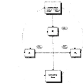
machines. The Petri net model we proposed to represent such process flow of each part type is called Process-Flow Model, which models the technological precedence constraints for processing parts and nor- mally provides more than one alternative route to accomplish the processing.

Now, an example will be given in the following to illustrate an FMS and as a example to construct its TPPN Model. The layout of this example is shown in Fig. 1. The part processing scenario is described as follows: there are two jobs, namely job J 1 and job

5 2 , which need to be carried out subjected to the job

requirements listed in Table 1. This table provides the technological precedence constraints among the operations. For example, J1 can be accomplished via two

process plans, P 1 1 and P 1 2 , where the former has three operations, 0 1 1 1 , 0 1 1 2 and 0 1 1 3 , and the latter has two operations, 0 1 2 1 and 0 1 2 2 . Whereas job JZ can be car- ried out only through single process plan consisting of two Operations, 0 2 1 1 and 0 2 1 2 . The operation 0 1 1 1 in process plan P 1 1 of job J 1 can be run by machine

M I at the cost of 2 minutes and can also be executed

by machine M 2 at the cost of 1 minute, the operation

0 1 1 2 can be run by machine M 2 at the cost of 3 min-

utes or by machine M 3 at the cost of 2 minutes, and the operation 0 1 1 3 can be executed by machine M I at the cost of 1 minute or by machine M 3 at the cost of 2 minutes. Note that in process plan 4 1 the operation

0 1 1 2 can be started only after the operation 0 1 1 1 is

completed.

3 GA Embedded Search over

a

Petri

Net in the Application for FMS

Genetic algorithm was developed by Holland [16] to study the adaptive process of natural systems and

Figure 1: The System Layout of Example

r--

I

Job 1

I

Job 2

I

Table 1: Job Requirements of Example

to design artificial system software that imitates the adaptive mechanism of the natural systems. The as- sumption underlying the use of GA's for scheduling is that optimal solutions will be found in the neighbor- hood of good solutions.

In general, GA consists of a chromosome representation of the nodes in the search space, a set of sim- ple operations that takes the current population into consideration and generates the successive improved population, a fitness function to evaluate the search nodes, and a set of stochastic assignments to control the genetic operations.

Notation

Before we explain how to apply the GA embedded search over a Petri net model, we will first introduce the following notation.

Conflict place: A place p E P with more than one output transitions, i.e., Ip

I

> 1.

List: A special type of list, denoted by 1 , of which each element is one kind of sequence of the identities of the output transitions associated with a conflict place to express a priority order of those transitions.

11111: The number of elements in the list 1.

ci: A chromosome, a set of Lists.

C: The set of all possible chromosomes, i.e., the search

space of a scheduling problem.

C,: The mating pool, tentative new population, for fur-

ther genetic operation.

n . ~ , : The total number of raw parts of a job Ji.

W I P : Abbreviation of "work in process", the total num- ber of parts remain in the system.

Te: The set of all enabled transitions for one marking.

Chromosome Representation

Since a TPPN model of an FMS has encoded each possible processing flow of every part type, i.e., has

(3)

modeled the technological precedence constrains for processing a part type, which usually allows more than one alternative route to accomplish the processing, we can extract a conflict place p , which corresponds to a ”plan selection” for a job, say job J,, from the TPPN model of an FMS and, then, create a list 1 , for tlhe place p , with 111,,

11

= n J , . Each element in the list 1 ,

is randomly assigned to one of the identities of the set

pp,.. Every time when a conflict place p , of this kind contains a token, we fire one, and only one, of its output transitions determined by the code recorded in tlhe list 1 , . Next, we create a list lpJ with

IIZ,, 11

= nJ, for a conflict place p , which corresponds to the ”resource assignment” for an operation of Job

J,

.

Each element of the list ZpJ is a sequence of the identities of those transitions in the set p, 0 to express a priority order of

those transitions. Every time when the place p , has a

token, we choose one of its enabled output transitions into the queue q ~ ,

,

registering all operations competing for the resource R,. Last, the representation of a schedule must be able to resolve the conflicts when there are several parts competing for one resource like machine, AGV, and a ticket of a path segment between two adjacent stops, etc. For each resource JR, with IR, 0

I

>

1, we find all operations using this resource R,, i.e., the set

R,.

and, then, create a list l ~ , with lllR.11 = W I P . Each element of the list

ZR,

is a

sequence of the identities of those transitions in the set R,. to express priority order of these transitions.

A chromosome is generated directly from the Petri net model, and is a set of lists, denoted by c = { l l , Z z , . . , I n } . In the following, we summarize the algo-

rithm of constructing a chromosome from a Petri net model.

Algorithm: (Chromosome Representation from

a Petri Net Model)

Step 1 : Chose a place p , E P with Ip. I > 1,

Step 2: If p , is corresponding to a plan selection of job J , , 1. create a list 1, with 111,11 = n j , ;

2. for each element of list l , , assign the identity of one

transition belonging to the set p , . randomly to it,

and goto Step 4 .

Step 3: If p , is corresponding to a resource assignment for an

operation of job J,,

1. create a list 1, with 111,11 = n j , ;

2. for each element of the list l , , assign a sequence of all elements in the set p , . to it randomly.

Step 4: If p , is corresponding a competition for a resource,

1. create a list 1, with 111,11 = W I P ;

2. for each element of the list l , , assign a sequence of all elements in the set p , . to it randomly.

Step 5: Repeat the above steps until every p , E P is visited.

Schedule Builder

A schedule builder is dedicated to transforming a chromosome to a feasible schedule and thus, we can

Figure 2: The Structure of Schedule Builder.

utilize it to evaluate the aforementioned indirect chromosome representation. Based on a Petri net model of the system, the evolution of the system can be described by the change of marking in the net. Fig. 2

shows the structure of the schedule builder. The firing sequence of transitions provides the order of the initiation of operations. In the following, we will describe how a schedule builder can use the chromosome to construct a feasible schedule over a Petri net model.

Algorithm: (Schedule Builder)

Step 1: Give an initial marking mo, and a chromosome ci E C ,

set the marking m = mo, where mo is some preset initial

marking, and set the pointer such that it points to the first

element of each list li.

Step 2: Find the set of all enabled transitions in the marking Step 3: If Te = 4,

m, namely, Te = {tl,t2,..,tn}.

1. find the minimum elapsing time such that one of the

busy resource is free;

2. find the maximum elapsing time such that all of the

busy resources are free;

3. update the time value between the minimum and

maximum elapsing time;

4. goto step 2.

Step 4 : Get an enabled transition ti E Te,

Step 5: If ti is corresponding to a plan selection for a job,

1. find the corresponding list l i E c;;

2. compare ti with t j which is currently pointed by the

3. if ti = t . , fire the transition ti, and update the

4. goto Step 4 .

pointer in the 1;;

pointer ofllist 1; to the next element;

Step 6: If ti is corresponding to the resource assignment for an operation,

1. find the corresponding list 1; E c;;

2 . set op; to ti according to the element, a priority order set, which is currently pointed by the pointer in the list 1 ; ;

3 . goto Step 4 .

Step 8: Put every opi to the queue QR; recording all enabled Step 9: For every queue q R i ,

(4)

1. find the corresponding list l ~ , E c,;

2. fire transition t, E I R , according to the element,

a priority order sequence set, which is currently

pointed by the pointer in the list I,;

3 . update the pointers of all lists relating to t , to the next element.

Step 10: Set m = ml, where mr is the current marking. Step 11: If the final marking has not been found, then goto Step

2.

Fitness

Function

The fitness function in genetic algorithms is typi- cally the objective function that we want to optimize in the problem. For the FMS scheduling problem, there exist several performance measures which can be used, such as maximum completion time of all jobs, i.e., makespan, percentage of jobs to meet the due dates, earliness or tardiness, the utilization of machines, or combinations of them. In the current implementation, first, we define the fitness evaluation for each chromosome as follow:

fi = "ax

-

mi

+

"in,

mmaZ = the maximum makespan for the current population.

mmin = the minimum makespan for the current population.

mi = the makespan of chromosome c, in the current popula-

Next, we use a linear scaling method t o scale the raw fitness value. We calculate the scaled fitness f t

from the raw fitness using a linear equation of the form:

f l = a * f + b .

In this equation, the coefficients a and b are usually

chosen to do two things: enforce equality of the raw and scaled average fitness values and cause maximum scaled fitness to be multi-times (usually twice) of the average fitness. These two conditions ensure that the average population members will receive one offspring copy which is also on average, but the best will receive the designated multiple number of copies [16].

where

tion.

Reproduction

The reproduction operator works on scaled fitness value. This operator, of course, is a n artificial ver- sion of natural selection, a Darwinian survival of the fittest among chromosome species.

In the implementation, we use the scheme where the probabilities of selection are calculated in the form pselecti = fi/Cfi. Then the expected number of chromosome ci, ei, is calculated ei = pselecti

*

populationsize. Samples of each chromosome are al- located, according to the integer part of the ei value, into the mating pool. The remainder of the chromosomes needed to fill the population in the mating pool are decided by the fractional parts. The fractional parts of the expected number values are treated as

probabilities where, for different chromosomes one by one, the weighted coin tosses are performed by tak- ing the fractional parts as the success probabilities for entering into the mating pool.

Crossover

The chromosome representation described above contains information about plan selections ,resource assignments of every operation, and resource competition resolutions. We can create new chromosomes by exchanging portions of two old chromosomes simply by using the following way.

Algorithm: (Crossover)

Step 1: Randomly select a pair of chromosomes ci E C, and

Step 2: For each list li E c i ,

cj E C, and create two new chromosomes c,/ and cjl.

1. get a corresponding list Ij E c j ;

2. toss a weighted coin as the success probability to

perform crossover; if it successs, then decides the crossover site cs; else set cs = llliII;

3 . assign each element of lists &I E C ~ I and l j l E cjl

to each element of lists li and l j separately and in

sequence before the crossover site cs;

4. assign each element of lists 1i1 E cil and I j l E cjt

to each element of lists Ij and l i separately and in

sequence after the crossover site cs.

Step 3: Evaluate the fitness value of the chromosome tit, and Step

4:

If the fitness value of cir is not better than that of ci, Step 5: If the fitness value of cjr is not better than that of cj, Step 6: Copy the contents of two old chromosomes ci and cj so

Step 7: Repeat the above steps until the whole chromosomes of the chromosome cjl by the schedule builder.

replace c i f by ci. replace cj I by cj .

that C ~ I = ci and c.1 = c '

successor population are constructed.

3 3 '

Mutation

Mutation can be considered as an occasional (with small probability) random alternation of the structure of a chromosome. One can think of mutation as an es- cape mechanism for premature convergence. The mutation operator selects a list li E ci and then changes each element value by tossing the weighted coin. In the implementation, the mutation is embedded into crossover operator, i.e., we modify the algorithm of the crossover operator so that the mutation operator is built into crossover process as follows.

0 For each element of each list I; E ci,

1. toss the weighted coin as success probability to do mutation;

2. if success, reset the element to a valid one randomly.

4

Search Based Dynamic FMS Sched-

uler

Due to the NP-complete nature of the scheduling problem of an FMS, one must inflict the exponential growth of search time with respect t o the problem size. Because the number of parts is high, the use of search techniques in the generation of a schedule for the complete set of parts is a heavy task. So, an approach

(5)

called adaptive scheduling [17], has been proposed for high-volume production problems with a new horizon- extension philosophy. The key idea underlying the proposed methodology consists of generating successive partial schedule, a complete schedule for a subset of total raw parts, as the production evolves, instead of generating a full schedule for all raw parts.

Dynamic

FMS

Scheduler

In our earlier research [18], a limited Work- In-Process (WIP), implementation of the adaptive scheduling algorithm [17], with an A* search based

scheduling method, has been proposed to solve the high-volume FMS scheduling problem. The implementation details are described as follows : First, it defines the WIP for the system. Second, it generates the total schedule segment by segment, of which each segment is a result of running the

A*

search, and each

A*

search is a full search from the current state (with the number of parts remaining in the system equal to maximum WIP) to a virtual goal state at which the processes of all involved parts are completed.

Now we propose a scheduling policy with the structure consisting of an automatic Petri-net generator, a Petri net model scheduler with GA embedding, a schedule generator, and an extension maker. We define the function of each component and the relations among them.

Automatic Petri net model generator : It gen-

erate a timed place Petri net model to describe the behaviors

of the part routings and the resource assignments from the file defining the capacity of every machine, possible plans for every job, the relations such as operation vs. machine and operation vs. time, the initial setup information including the starting time, and run time informations of every job, like the number of total raw parts of a job and job priority.

Petri net model scheduler with GA embedding

: Based on the Petri-net model generated by the Petri-net gen-

erator, it finds a near-optimal schedule in the form of a list of n decisions from the current state to a virtual goal at which the involved parts are completed.

Schedule generator : It generates a partial schedule for

a mix of different job types till some of them may meet some

predefined condition, and for every job its schedule simply corresponds to the firing sequence over Petri net model, and hence

it is dynamic in the sense that the scheduler can re-adjust its

previous schedule to adapt to the new system state.

Extension maker :

some extension criteria from the current system state. It creates the next search segment by

Implement

at

ion

In this subsection, we present the implementation of the proposed dynamic FMS scheduler. First, we define WIP and the condition for the schedule generator, which generates the partial schedule in the current segmented GA search for every job. Before that, three involved parameters are first defined in the following.

Definition 4.1 qJ stands for the upper bound of the WIIP of job J j in each G A segment search.

Definition 4.2 0 j is the lower bound of the finished parts of

job J j for a G A segment search.

Definition 4.3 Ai denotes the number of finished parts of job

J j for a G A segment search.

For each segmented

GA

search,

9j

is the initial WIP of job Jj. That is to say, before a segment search

starts, the number of parts of job Jj in the FMS must be increased to match ! P j . The search goal is that every parts in this search are completely processed and are moved out the system. The GA search will then find optimal firing sequences according to the given evaluation function, whereby a part of schedule can be generated. But when the system state evolves to a condition in which Aj 2 0 j for every j , the schedule

generation will be halted at that point, and another similar segmented GA search will be initiated again and the number of all the residing parts will all be increased to the respective upper bound, namely ! P j .

In the following, we summarizes the procedures of the dynamic scheduling described above.

Algorithm: (Dynamic Scheduling Algorithm)

Step 1: For each uncompleted job J 3 , set the number of parts Step 2: Create a GA segment search to a get firing sequence.

Step 3: Get a transition t from the firing sequence. Step 4 : Fire the transition t in the TPPN Model.

Step 5: Output a proper schedule command associated with Step 6: Repeat Step 3, Step 4 and Step 5 until every uncom- Step 7: Repeat the above steps until all jobs have been com-

Although, the dynamic scheduling strategy may not provide an optimal schedule, when the number of parts to be processed is very high, it can generate an effec- tive schedule in a shorter time interval. In additional, the parameter !P and 0 can be used t o assign priority to every job. Because 9 s are used to assign number of parts of every job in a segment search, a greater

!PJ means that the job J, should have more chances in getting system resources Further, 0 s are used to bound the number of finished parts of every job in each segment search, i.e., the minimum number of finished parts of job JJ in a segment search can be no

smaller than 0,. For example, there are two jobs in the system, J1 and J2 with ! P I = 8 and q 2 = 4, that is to say, for each segment search, there are 8 parts of

J1 and

4

parts of J2, and hence J1 has more oppor-

tunity t o resource allocation than J2. Now if 01 = 3

and 0 2 = 1, then the dynamic scheduling algorithm

promises that every segment search produce at least 3 parts for J1 and 1 parts for J2. As a result from the

fact that !PI

>

!P2 and 01

>

0 2 , one can generate a schedule in which J1 appears t o have higher prior-

ity than Jz. In the extreme condition O1

>

@ 2 and

0 2 = 0, one can guarantee that 51 will always finished

before J2.

in system of job J3 to match \k,

.

the transit ion.

pleted job J3 meets the condition AJ >= 0,.

(6)

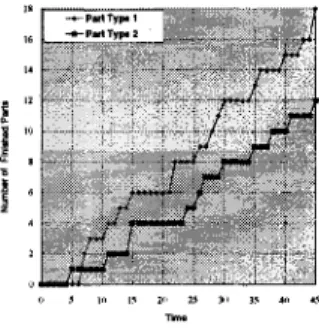
Figure 3: The Relation of Finished Parts and Time for the Example

Example

:

FMS

Scheduling Problem

The layout of the FMS is show in Fig 1 and the

job requirements for this example is shown in Table 1. The total number of parts and the priorities of jobs are both shown in the following. In each segmented GA embedded search, the initial WIP of the system is set to be 10.

The total number of job J1 = 18

0 The total number of job J2 = 12

The GA used the following parameters throughout

population size = 30

crossover probability = 0.7

0 mutation probability = 0.05

maximum number of generation = 100

In Fig 3, the relation between the number of completed parts and the completion time are shown. In average, each segment GA embedded search takes about 3 minutes for one trial on PC 486.

$1 = 6 , 0 1 = 4 $2 = 4 , 0 2 = 3

the simulations.

5 Conclusion

In this paper, we consider the FMS scheduling problem. We first use a systematic Petri-net modeling for an FMS, which is composed of two sub-models, Trans- portation Model and Process-Flow model. Based on this complete Petri net model, a GA embedded search method was applied. The representation of the search nodes (schedules) used in GA is in the form of lists to resolve conflicts for each conflict place in the TPPN model of an FMS. By the genetic search algorithm, a path from the initial marking to the final marking in the reachability graph, generated by the firing rule of the Petri net can be found. This facilitates us to de- velop a dynamic scheduling method incorporating the GA search. It not only generates an efficient schedule but also allows one to set the different priorities among the jobs. Our experiments show that this approach does represent a good alternative over other techniques for this class of problems.

References

J. H. Blackstone, D. T. Phillips, and G. L. Hofg, “A state- of-the-art survey of dispatching rules for manu acturing job

shop operations,” Int. J . Productzon Res., vol. 20, no. 1,

H. Fujimoto, K. Yasuda, Y. Tanigawa, and K. Iwahashi, “Applications of Genetic Algorithm and simulation to dis-

patching rule-based FMS scheduling,” in IEEE Int. Conf.

on Robotzcs and Automatzon, pp. 190-195, 1995.

H. Fujimoto, K. Yasuda, and T. Ishimaru, “Evaluation of

scheduling rules in FMS using simulator,” in Proceedzngs

of the JAPAN/USA Symposaum on Flexible Automation,

H. Shih and T. Sekiguchi, “A timed Petri net and beam

search based on-line FMS scheduling system with routing flexibility,” in Proc. IEEE Int. Conf. on Robotzcs and Au- tomation, pp. 2548-2553, Apr. 1991.

D. Y. Lee and F. DiCesare, “Scheduling flexible manufac-

turing systems using Petri nets and heuristic search,” IEEE

Pansaction on Robotzcs and Automation, vol. 10, pp. 123-

132, Apr. 1994.

C.-J. T., L.-C. F., and Y.4. H., “Modeling and simula-

tion for flexible manufacturing systems using Petri net,” in Proc. 2nd. Int. Conf. on Automation Technology, pp. 31-

38, 1992.

D. Whitley, T. Starkweather, and D. Fuquay, “Scheduling

problems and traveling salesman: The genetic edge recom- bination operator,” in Proc. 3rd Int. Conf. on Genetzc Al- E. Falkenauer and S. Bouffouix, “A Genetic Algorithm for

job shop,” in Proc. IEEE Int. Conf. on Robotzcs and Au-

tomatron, pp. 824-829, Apr. 1991.

H.-L. Fang, P. Ross, and D. Corne, “A promising Genetic

Algorithm to job-shop scheduling, rescheduling, and open- shop scheduling problems,” in Proc. 5th Int. Conf. on Ge- netic Algorithms, pp. 375-382, 1993.

R. Nakano and T. Yamada, “Conventional Genetic Algo-

rithm for job shop problems,” in Proc. 4th Int. Conf. on

Genetrc Algorithms, pp. 474-479, 1991.

S. Kobayashi, I. Ono, and M. Yamamura, “An efficient

Genetic Algorithm for job shop scheduling problems,” in Proc. 6th Int. Conf. on Genetic Algorzthms, pp. 506-511,

1995.

J. F. Muth and G. L. Thompson, Industrzal Scheduling. Englewood Cliffs, N. J.: Prentice-Hall, 1963.

T.-H. Sun, C.-W. Cheng, and L.-C. Fu, “A Petri net based

approach to modeling and scheduling for an FMS and a case study,” IEEE Trans. on Industrral Electronics, vol. 41, pp. 593-600, Dec. 1994.

D. Y. Lee and F. DiCesare, “Integrated scheduling of flex-

ible manufacturing systems employing automated guided

vehicles,” IEEE Trans. on Industrial Electronics, vol. 41,

pp. 602-610, Dec. 1994.

D. Y. Lee and F. DiCesare, “Integrated models for schedul-

ing flexible manufacturing systems,” in Proc. IEEE Int.

Conf. on Robotzcs and Automatzon, pp. 827-832, 1993. J. Holland, Adaptatzon zn Natural and Artijical Systems. Ann Arbor, MI: University of Michigan Press, 1975. C. F. Bispo, 3. J. Sentieiro, and R. D. Hibberd, “Adap-

tive scheduling for high-volume Shops,” IEEE Trans. on

Robotzcs and Automation, vol. 8 , pp. 696-706, Dec. 1992. P. S. Liu and L. C. Fu, “Hierarchical dynamic scheduling for an FMS,” in Proc. 3rd. Int. Conf. on Computer Integrated Manufacturang, pp. 393-402, May 1992.

pp. 27-45, 1982.

vol. 2, pp. 1143-1146, 1992.

gonthms, p ~ . 133-140, 1989.