Value at risk of life insurance policy reserves

(1)

Value at Risk of Life Insurance Policy Reserves (壽險保單準備金之風險值)

Chenghsien Tsai a (蔡政憲)

Department of Risk Management and Insurance (風險管理與保險學系) National Chengchi University (國立政治大學)

Weiyu Kuo (郭維裕)

Department of International Trade (國際貿易學系) National Chengchi University (國立政治大學)

Mengyi Li (李孟倚) Actuarial Department (精算部)

Allianz President Insurance (統一安聯人壽保險公司)

Abstract

We estimate the value at risk (VaR) of life insurance policy reserves in this paper. Since the market price of reserves does not exist, we construct a simulation model considering

mortality rate risk, interest rate risk, surrender rate risk, and parameter estimation risks to estimate the VaR. Simulation results show that the VaR from mortality rate risk is small but interest rate risk as well as the parameter estimation risk of interest rate model significantly enlarges the VaR. On the other hand, surrender rate risk reduces reserve VaR. With regard to individual product, annuity and whole life insurance have the largest VaR, followed by pure endowment and endowment. Term life insurance has the smallest one.

Keywords: Value at risk; Policy reserves; Life Insurance

摘要作者們於本文中估計數種保險商品準備金之風險值。由於準備金沒有市場價格，作者們建立了一個包含死亡率風險，利率風險，解約率風險，以及參數估計風險的模擬模型來估計風險值。我們發現死亡率所產生的風險值很低，利率風險以及利率模型的參數估計風險會使風險值顯著變大，而解約率風險則會降低準備金的風險值。保險商品中，年金與終身壽險的風險值最大，生存險與生死合險次之，而定期壽險的風險值則最小。關鍵詞：風險值、保單準備金、人身保險 I. Introduction a

Corresponding author. Address: No. 64, Section 2, Chihnan Road, Taipei, Taiwan 11623; tel.:

+886-2-2936-9647; fax: +886-2-2939-3864; e-mail: ctsai@nccu.edu.tw. The author thanks National Science Council for its financial support (project number: 89-2416-H-004-069).

(2)

The use of value at risk (VaR) exploded in banking and securities industries during the

last decade. It is becoming universal in the private sector (Dowd, 1998, p.19 – 20). In

addition to getting popular in the private sector, VaR is gaining acceptance from regulators.

For instance, the Basle Committee allowed certain banks to use their own VaR models in

calculating required capital starting from 1997.

VaR is important to the insurance industries as well. Firstly, VaR can deal with

underwriting and financial risks at the same time. It can cover risk factors embedded in the

liabilities as well as the assets of an insurance company. It is also able to take into account

the correlations among insurance lines, the correlations among invested assets, and the

correlations between liabilities and assets.

Secondly, the trend of financial services integration will make VaR indispensable to

the insurance industry. The integration among financial services industries brings the

insurance company to compete with other financial institutions head to head in many aspects

including risk management. Since VaR is a well-developed risk management system and

has been adopted by many financial institutions, insurance companies will have to develop

their own VaR systems to effectively manage their risks to remain competitive.

Thirdly, insurance regulators will probably adopt VaR in capital requirements. Bank

regulators have accommodated VaR in addition to the Standardized method. Since the

(3)

risk-based capital requirements currently used in the insurance industries are similar to the

standardized method, insurance regulators might follow the track of bank regulators and

adopt VaR in the future. Indeed, the International Association of Insurance Supervisors

(IAIS) declares in the Principles on Capital Adequacy and Solvency “[insurance] supervisors

may consider the use of internal capital models as a basis for a capital requirement.”

Albeit the popularity and importance of VaR, we find only one paper studying VaR in

the insurance literature. Panning (1999) identified two risk factors for property-casualty

insurers’ loss reserves: payout pattern and inflation. Panning used a regression model to

decompose loss reserves into a loss growth function and a payout pattern function. From

the variance-covariance matrix of the estimated parameters in these two functions, he was

able to conduct Monte Carlo simulation to generate the distribution of loss reserves’ present

value and obtained VaR from this distribution.

Since no one has applied VaR to the liabilities of life insurance companies, we

establish a valuation model and carry out Monte Carlo simulation to calculate the VaR of

policy reserves for several life insurance products in this paper. To establish such a model

we need to identify and model risk factors. The identified risk factors include mortality rate

risk, interest rate risk, and surrender rate risk. The first two are easy to spot because

mortality rates affect future cash flows and interest rate determines the discounting.

(4)

contracts a provision that grants the policyholder who elects to terminate the policy the right

to a cash surrender value. The exercise for the surrender option would result in cash

payments and decreases future premium income for life insurance companies. In addition, it

would make the cash flows of life insurance be sensitive to the interest rate. Several recent

actuarial studies in the Transactions of Society of Actuaries Reports documented that

policyholders tend to surrender policies to reinvest in higher-yield alternatives as interest rate

rises.1 We also observed record numbers of surrenders during the high interest rate period

of the 1980s.

The sensitivity of the cash flows to the interest rate could significantly alter the

distribution of reserves. Babbel (1995), Briys and Varenne (1997), and Santomero and

Babbel (1997) found that the sensitivity was critical to the duration and convexity of the

insurance policy. Misspecifications about the sensitivity could cause large errors in the

estimates of effective duration and even greater errors in the estimates of convexity. The

disintermediation that happened to the U.S. life insurers during the 1980s also demonstrated

the adverse effect of interest-rate-sensitive surrenders. Many life insurers experienced

negative cash flows for the first time since the 1930s’ depression and were forced to liquidate

assets at depressed prices (Black and Skipper, 2000, p. 111). The consideration of

interest-rate-sensitive surrender behavior is therefore crucial to the estimation for VaR.

1

For instance, Cox, Laporte, Linney, and Lombardi (1992) and the Annuity Persistency Study in the 1995-96 reports (p. 559-638).

(5)

We calculate the VaR associated with mortality rate risk by the standard deviations of

mortality rates derived within a binomial framework. To quantify interest rate risk, we

employ the term structure model of the interest rate developed by Vasicek (1977) in which

the instantaneous spot interest rate follows a mean-reverting Ornstein-Uhlenbeck process.

To evaluate surrender rate risk, we establish a linear regression model of surrender rate to

capture the relation between interest rate and surrender rate. We further consider the

parameter estimation risk of the interest rate and surrender rate models. To assess the

accuracy of our estimated VaRs, we use the kernel estimation method to estimate the

confidence intervals of the VaRs. The above analyses are applied to endowment insurance,

pure endowment insurance, term life insurance, whole life insurance, and deferred whole life

annuity.

Our results show that the VaR generated from mortality rate risk is insignificant while

the VaR from interest rate risk is substantial. These results are consistent with the

observation that life insurers suffer more from interest rate risk than from mortality rate risk.

On the other hand, the marginal contribution of surrender rate risk to VaR is negative. This

result is understandable when we realize that the surrender option is analogue to the

prepayment option in loans that has been shown to be able to decrease the effective duration.

Such a result implies that life insurers would overestimate the VaR of insurance and

(6)

We also find that the parameter risk of the interest rate model is considerable. With regard

to product risk, annuity and whole life insurance have the largest VaR, term life insurance has

the smallest one, and pure endowment and endowment insurance have medium VaRs.

This paper contributes to the literature in several aspects. First, we consider both

stochastic interest rate and surrender rate when calculating the reserve VaR for several types

of life insurance products. Second, we examine the impact on reserve VaR from several risk

factors, including mortality rate, interest rate, surrender rate, and parameter estimation risk.

Finally, we document the beneficial effect of surrender options on reserve VaR, which has

implications to life insurer’s risk management.

This paper consists of six sections. Following this introduction section is the

simulation setting section in which we describe the set up of the simulation. We then

analyze the reserve VaR for several types of life insurance from the identified three risk

factors one after another. The accuracy check on the estimated VaR is provided in each

section. The last section contains conclusions and discussions for future researches.

II. Simulation Setting

Consider a group of N life-aged-x policyholders. Assume that these policyholders

have two causes of decrement: mortality and early surrender. For each of these

policyholders, the probability of death and surrender in policy year t (t ≥1) are specified by ) ( 1 m t x

(7)

endowment, T-year term life, whole life, and T-year deferred whole life annuities are

available to these policyholders with net level annual premium of $P payable at the beginning

of surviving years for at most T years. Let Fend, Fterm, and Fwhole be the death benefits of the

endowment, term life, and whole life insurance payable at the end of the death year or at the

end of the year x+T, Fpure be the living benefit of pure endowment insurance payable at the

end of the year x+T if the policyholder survives, and Fann be the annual payment of the

annuity payable at the beginning of surviving years. If policyholders surrender their policies

during policy year t, they receive the amount of _tS at the end of the year, where the i_x up-script i denotes the type of policy. We assume that

i x t i x t V T t S ⎟× ⎠ ⎞ ⎜ ⎝ ⎛ ₊ _× = 0.8 0.2 if t<T

= _tV if t≧T _xi (for whole life insurance and annuity),

(1)2

where _tV is the policy reserve at the end of policy year t calculated using random future _xi lifetime and deterministic interest rate as in the chapter 7 of Bowers et al. (1986). Let Lend,

Lterm, Lwhole, Lpure, and Lann be the random variable denoting the present value of the cash

flows generated by these insurance policy pools, respectively. Then

(

)

(

)

[

]

{

}

T T x end T t t t x t t x (l) t x end x t t x (m) t x end end v l F v l P v l q S l q F L × × + × × − × × × + × × = + = +− +− +− +− +− −

∑

1 1 1 1 1 1 1 , (2) 2

The formula comes from the Model Life Insurance Policy Provisions of Taiwan. It possesses the general property of surrender charges: high at the beginning and descends as the policy matures.

(8)

(

)

[

]

{

}

pure x T T T t t t x t t x l t x pure x t pure S q l v P l v F l v L = × × × − × × + × ₊ × = +− +− +− −

∑

1 1 1 1 ) ( 1 ,

(

)

(

)

[

]

{

}

∑

= +− +− +− +− +− − × × − × × × + × × = T t x t t x t t (l) t x term x t t x (m) t x term term F q l S q l v P l v L 1 1 1 1 1 1 1 ,

(

)

(

)

[

]

{

}

_∑

∑

= +− − − = +− +− +− +− × × − × × × + × × = T t t t x x t t t x (l) t x whole x t t x (m) t x whole whole F q l S q l v P l v L 1 1 1 1 1 1 1 1 ω ,

(

)

[

]

∑

= +− − − = + − − = +− +− × × − × × + × × × = T t t t x x ω T t ann x T t x ω t x t t (l) t x ann x t ann v l P v l F v l q S L 1 1 1 1 1 1 1 ,

where l_x_+t₋₁ is the number of survivors at the beginning of policy year t,

(

()

)

1 ) ( 1 1 1 l t x m t x t x t x l q q l ₊ = ₊₋ × − ₊₋ − ₊₋ , (3) t

v is the discount factor for the cash flows at time t,

(

)(

) (

_t

)

t _r _r _r v + + + = 1 1 1 1 2 1 L , (4)

rt is the interest rate in policy year t, and

ω is the largest age in the mortality table.3

The random variable L represents the present value of insurers’ liabilities associated

with pools of policies at the time when the policies are sold. The statistical properties of L

are critical to the risk management of reserves and are of great concerns to actuaries,

insurance regulators, and various stakeholders of insurance companies. Our goal is to

estimate the distribution and VaR of L.4

3

Notice that l_x = N and v₀ = 1.

4

The time horizon for the VaR of L is the coverage period of the policy because the uncertainty of L comes from the uncertainty in the timing of benefit payments and the interest rate over the entire policy life. For

(9)

In the following simulation, we specify that N =100,000, T =20, P=27.133, 000 , 1 = end

F , F_pure =1,110, 067F_term =10, , 917F_whole =2, , 86F_ann = , x=30, and

100 =

w .5 In addition, q(_xm₊_t)₋₁ is assumed to be distributed as the 1980 CSO male mortality table and the interest rate used in calculating _tV is 6%. We ignore dividends, expenses, _xi loadings, taxes, and new business in the simulation.

III. Mortality Rate Risk

Our focus in this section is on the risk arising from the uncertainty of mortality rates.

We thus assume that the interest rate is fixed at 6% and there are no early surrenders in this

section. When assessing mortality rate risk, we recognize that the number of deaths d_x_+t₋₁ = q_x(m₊_t)₋₁×l_x₊_t₋₁ follows a binomial distribution with parameters l_x_+t₋₁ and q(_xm₊_t)₋₁. Hence,

] | ˆ [ 1 ) ( 1 +− − + x t m t x l q E = 1 [ 1] 1 − + ∧ − + t x t x d E l = ) ( 1 m t x q ₊₋ , and (5) ] | ˆ [q(_x₊m_t)₋₁ l_x₊_t₋₁ Var = ₂1 [ ₁] 1 − + − + t x t x d V l = 1 ) ( 1 ) ( 1(1 ) − + − + − + − t x m t x m t x l q q (6)

Since we do not observe q_x(₊m_t)₋₁, we replace it with the estimate qˆ(_xm₊_t)₋₁. Moreover, when l_x_+t₋₁ is large, qˆ_x(₊m_t)₋₁ is distributed approximately as a normal distribution with mean

) ( 1 ˆ_xm_t q ₊₋ and variance 1 ) ( 1 ) ( 1(1 ˆ ) ˆ − + − + − + − t x m t x m t x l q q .

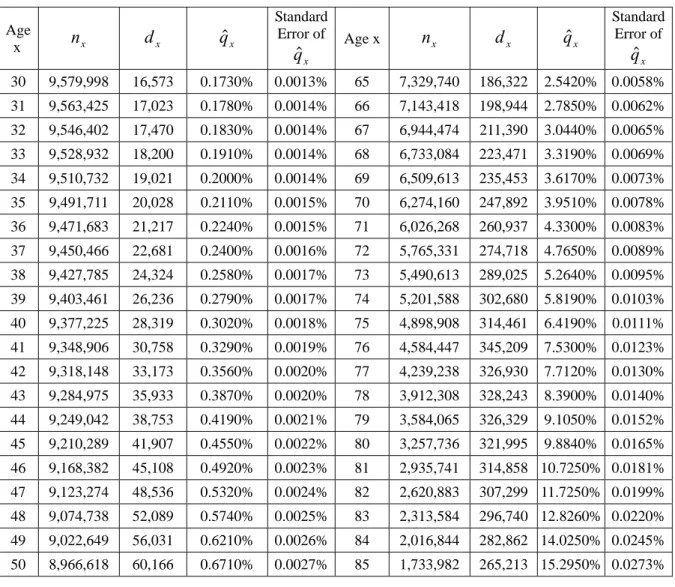
We then compute the VaR associated with mortality rate risk by the following steps.

First, the standard errors of mortality rates are calculated. The results are in Table 1.

Second, we assume that mortality rates are normally distributed with parameters estimated

instance, the risk of Lend originates from the uncertain cash flow (determined by uncertain mortality rate and

surrender rate) and uncertain interest rate in the future 20 years. Therefore, the time horizon for Lend’s VaR is

(10)

from the 1980 male CSO table. Third, we draw randomly a set of mortality rates from the

above normal distributions and use them to calculate the number of deaths in every policy

year. Fourth, cash inflows and outflows in every policy year are calculated according to the

number of deaths and survivors. Fifth, under the assumption of fixed interest rate and zero

surrender we calculate the policy reserve. We repeat step 3 to 5 for 10,000 times to

construct the distribution of policy reserves and then estimate VaR. Our VaR is an absolute

VaR and is defined as the 95th percentile of the simulated policy reserve distribution.

Table 1: Statistics of Mortality Rates

Age x nx dx qˆx Standard Error of x qˆ Age x nx dx qˆx Standard Error of x qˆ 30 9,579,998 16,573 0.1730% 0.0013% 65 7,329,740 186,322 2.5420% 0.0058% 31 9,563,425 17,023 0.1780% 0.0014% 66 7,143,418 198,944 2.7850% 0.0062% 32 9,546,402 17,470 0.1830% 0.0014% 67 6,944,474 211,390 3.0440% 0.0065% 33 9,528,932 18,200 0.1910% 0.0014% 68 6,733,084 223,471 3.3190% 0.0069% 34 9,510,732 19,021 0.2000% 0.0014% 69 6,509,613 235,453 3.6170% 0.0073% 35 9,491,711 20,028 0.2110% 0.0015% 70 6,274,160 247,892 3.9510% 0.0078% 36 9,471,683 21,217 0.2240% 0.0015% 71 6,026,268 260,937 4.3300% 0.0083% 37 9,450,466 22,681 0.2400% 0.0016% 72 5,765,331 274,718 4.7650% 0.0089% 38 9,427,785 24,324 0.2580% 0.0017% 73 5,490,613 289,025 5.2640% 0.0095% 39 9,403,461 26,236 0.2790% 0.0017% 74 5,201,588 302,680 5.8190% 0.0103% 40 9,377,225 28,319 0.3020% 0.0018% 75 4,898,908 314,461 6.4190% 0.0111% 41 9,348,906 30,758 0.3290% 0.0019% 76 4,584,447 345,209 7.5300% 0.0123% 42 9,318,148 33,173 0.3560% 0.0020% 77 4,239,238 326,930 7.7120% 0.0130% 43 9,284,975 35,933 0.3870% 0.0020% 78 3,912,308 328,243 8.3900% 0.0140% 44 9,249,042 38,753 0.4190% 0.0021% 79 3,584,065 326,329 9.1050% 0.0152% 45 9,210,289 41,907 0.4550% 0.0022% 80 3,257,736 321,995 9.8840% 0.0165% 46 9,168,382 45,108 0.4920% 0.0023% 81 2,935,741 314,858 10.7250% 0.0181% 47 9,123,274 48,536 0.5320% 0.0024% 82 2,620,883 307,299 11.7250% 0.0199% 48 9,074,738 52,089 0.5740% 0.0025% 83 2,313,584 296,740 12.8260% 0.0220% 49 9,022,649 56,031 0.6210% 0.0026% 84 2,016,844 282,862 14.0250% 0.0245% 50 8,966,618 60,166 0.6710% 0.0027% 85 1,733,982 265,213 15.2950% 0.0273% 5

(11)

51 8,906,452 65,017 0.7300% 0.0029% 86 1,468,769 243,948 16.6090% 0.0307% 52 8,841,435 70,378 0.7960% 0.0030% 87 1,224,821 219,917 17.9550% 0.0347% 53 8,771,057 76,396 0.8710% 0.0031% 88 1,004,904 194,218 19.3270% 0.0394% 54 8,694,661 83,121 0.9560% 0.0033% 89 810,686 168,031 20.7270% 0.0450% 55 8,661,540 90,163 1.0410% 0.0034% 90 642,655 142,522 22.1771% 0.0518% 56 8,521,377 97,655 1.1460% 0.0036% 91 500,133 118,522 23.6981% 0.0601% 57 8,423,722 105,212 1.2490% 0.0038% 92 381,611 96,719 25.3449% 0.0704% 58 8,318,510 113,049 1.3590% 0.0040% 93 284,892 77,522 27.2110% 0.0834% 59 8,205,461 121,195 1.4770% 0.0042% 94 207,370 61,361 29.5901% 0.1002% 60 8,084,266 129,995 1.6080% 0.0044% 95 146,009 48,177 32.9959% 0.1231% 61 7,954,271 139,518 1.7540% 0.0047% 96 97,832 37,621 38.4547% 0.1555% 62 7,814,753 149,965 1.9190% 0.0049% 97 60,211 28,913 48.0195% 0.2036% 63 7,664,788 161,420 2.1060% 0.0052% 98 31,298 20,593 65.7965% 0.2682% 64 7,503,368 173,628 2.3140% 0.0055% 99 10,705 10,705 100% 0%

Since our VaR is a statistical estimate based on simulated distributions, we should

assess its precision using certain measures such as the width of the confidence interval. We

estimate the 95% confidence interval for our VaR by order statistics described in the

following.

Let Y1 < Y2 < … < Yn be the order statistics of a random sample of size n from a

continuous-type distribution and let π_p denote the (100p)th percentile of the distribution. According to the section 10.2 in Hogg and Tanis (1997), the 100(1-α)% confidence interval

for the unknown π_p can be derived using the following equation: α − 1 = P(Y_i <π_p <Y_j) = k n k j i k p p k n k n − − = − −

∑

(1 ) )! ( ! ! 1 = ) ) 1 ( 5 . 0 ( ) ) 1 ( 5 . 0 ( ) 5 . 0 5 . 0 ( p np np i p np np j j W i P − − − Φ − − − − Φ ≈ − < < − , (7)

where 1≤i< j ≤n, W is binomially distributed with mean np and variance np(1-p), and Φ is the cumulative normal distribution function. Once the samples are observed and the pair

(12)

(i, j) determined, the interval (Yi, Yj) could serve as a 100(1-α)% confidence interval for π_p.

Since equation (7) contains two unknown numbers, more than one pair of (i, j) can

satisfy the equation. To assure the uniqueness of the confidence interval, we impose an

additional constraint: the confidence interval should be as symmetric around π_p as possible. More specifically, (i, j) are chosen so that

p n j n i p− = − . (8) We specify that α = 0.05, p = 0.95, and n = 10,000 in this paper.

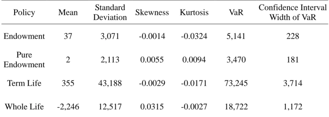
The simulation results for mortality rate risk are in Table 2. They indicate that the

mortality rate risk defined in this paper is immaterial for all types of policies. Compared to

annual premiums of $2,713,300, the VaRs of policies are insignificant. The insignificance is

due to the small standard deviations of mortality rates that result from the large size of the

insurance pool. The estimated VaRs have satisfactory accuracy since the widths of

confidence intervals are about four to eight percent of the VaRs.

Table 2: Mortality Rate Risk (MR)

Policy Mean Standard

Deviation Skewness Kurtosis VaR

Confidence Interval Width of VaR Endowment 37 3,071 -0.0014 -0.0324 5,141 228 Pure Endowment 2 2,113 0.0055 0.0094 3,470 181 Term Life 355 43,188 -0.0029 -0.0171 73,245 3,714 Whole Life -2,246 12,517 0.0315 -0.0027 18,722 1,172

(13)

Annuity -9,243 3,476 -0.0216 0.0134 -3,501 300

IV. Interest Rate Risk 1. The Term Structure Model and Its Estimation

In this section we incorporate an additional risk factor into the simulation: interest rate.

To capture the dynamics of interest rate, we employ the term structure model developed by

Vasicek (1977) and use statistical approaches to estimate the parameters of the model from

historical interest rates. Vasicek’s model assumes that the instantaneous spot rate follows a

mean-reverting Ornstein-Uhlenbeck process:

t t

t q m r dt vdW

dr = ( − ) + , (9) where W is a Wiener process, _t m is the long-run average of spot rates, q reflects the speed of mean reverting, and v is the volatility of the process. The Vasicek’s model has a discrete AR(1) counterpart that is frequently used in the actuarial literature such as Beekman

and Fuelling (1990; 1993), Parker (1994; 1997), and Marceau and Gaillardetz (1999).

The statistical method used to estimate the parameters of Vasicek’s model is from

Duan (1994). Assuming that the instantaneous spot rate follows equation (9), Duan derived

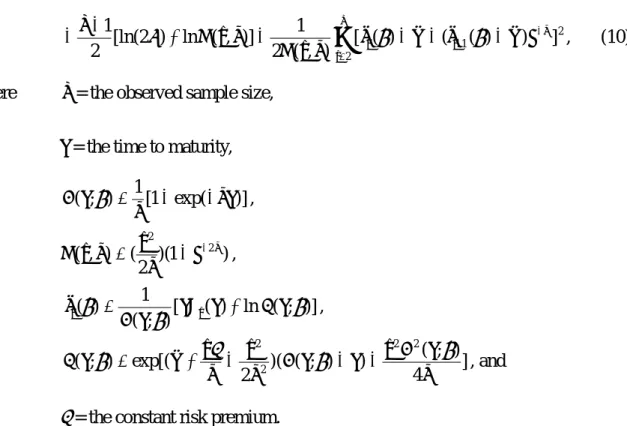
the log-likelihood function in terms of the observed interest rates:

L(Rt(k), t = 1, 2, …, n; θ)

(14)

2 1 2 ] ) ) ( ( ) ( [ ) , ( 2 1 )] , ( ln ) 2 [ln( 2 1 q t n t t e m r m r q v V q v V n − − = − − − − + − − π

∑

) θ ) θ , (10)

where n = the observed sample size,

k = the time to maturity,

)] exp( 1 [ 1 ) ; ( qk q k B θ = − − , ) 1 )( 2 ( ) , ( 2 2 q e q v q v V ₌ ₋ − , [ ( ) ln ( ; )] ) ; ( 1 ) ( θ θ θ kR k A k k B r)_t = _t + , ] 4 ) ; ( ) ) ; ( )( 2 exp[( ) ; ( 2 2 2 2 q k B v k k B q v q v m k A θ = + λ − θ − − θ , and

λ = the constant risk premium.

The data used for the estimation are the monthly rates of one-year U.S. Treasury bills

from January 1960 to March 1999.6 We use GAUSS to do the numerical optimization.

The estimation results for the parameters are in Table 3.7

Table 3: Estimated Parameters of the Term Structure Model

Parameter Estimate Standard

Error p-value

Correlation Matrix of Estimated Parameters

q 0.0151 0.0080 0.0293 1.000 -0.012 0.239

m 0.0602 0.0120 0.0000 -0.012 1.000 -0.003

v 0.0040 0.0001 0.0001 0.239 -0.003 1.000

2. Simulation of Interest Rates and L

6

We collect the data from the web site of Federal Reserve Bank of Minneapolis. The web site address is " http://minneapolisfed.org/economy/usindex.html." Interest rates are calculated based on ask quotations and then transformed to annualized continuously compound rates.

7

The results in Table 3 are obtained under the assumption that λ is zero because the preliminary maximum likelihood estimation involving four parameters shows that λ is not significantly different from zero.

(15)

We simulate 10,000 interest rate paths of monthly one-year T-bill rates for seventy

years using 6% as the initial value.8 Combining the 10,000 interest rate paths with the

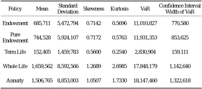
10,000 sets of l_x_+t₋₁ simulated in Section III, we obtain the distribution of L under the consideration for stochastic interest rate as well as random mortality rates. The results are

shown in Table 4.

Table 4: Interest Rate Risk (IR) + MR

Confidence Interval Width of VaR Endowment 685,711 5,472,794 0.7142 0.5696 11,010,827 770,580 Pure Endowment 744,528 5,924,107 0.7172 0.5763 11,931,353 853,625 Term Life 152,405 1,459,783 0.5600 0.2540 2,830,904 159,111 Whole Life 1,659,562 8,592,566 1.2689 2.6985 17,848,179 1,142,640 Annuity 1,506,765 8,853,003 1.0507 1.7330 18,147,460 1,322,618

The interest rate risk is momentous for all types of policies. The VaRs of whole life

insurance and deferred annuity are more than six times of annual premiums and the VaRs of

endowment and pure endowment policies are more than four time of annual premiums.

Even term life insurance has a VaR larger than annual premiums. These figures suggest that

the insurer has to keep low premium-to-surplus ratio and tremendous amount of surplus to

Following Duan (1994), we re-estimate the other three parameters under the assumption that λ is zero.

8

(16)

maintain an acceptable solvency probability.

The large VaRs result from the possibilities of low interest rates and the long-term

nature of policies. When interest rates are low, the present value of the insurer’s future

obligation increases. The long maturity of the insurance aggravates such effect and makes

reserves much larger than expected. Whole life insurance and annuity have the largest VaRs

because they have the longest expected maturities. Endowment and pure endowment

policies have larger VaRs than term life because they have larger expected payments toward

the end of the contracts. Pure endowment has a slightly larger VaR than endowment

because it pays living benefits at the end only and thus has higher percentage of cash

outflows incurred later. The substance of interest rate risk versus the insignificance of

mortality rate risk is consistent with the literature and the experience of the life insurance

industry.

3. Parameter Estimation Risk of the Interest Rate Model

To evaluate the parameter estimation risk, we first use the covariance matrix resulting

from the estimation for the interest rate model to generate sets of parameters. Specifically,

we assume that the parameters

(

qˆ,mˆ,νˆ

)

are from a multivariate normal distribution with expected values and covariance matrix as specified in Table 3. We then draw 10,000 sets of

(

qˆ,mˆ,νˆ

)

from this multivariate normal distribution. For each of these 10,000 sets of

(17)

parameters, we simulate one interest rate path and get 10,000 paths altogether.9 Combining

these interest rate paths with the 10,000 sets of l_x_+t₋₁ simulated in Section III, we obtain the distribution of L under random mortality rates, stochastic interest rate, and parameter

estimation errors of the interest rate model. Relevant results are in Table 5.

Table 5: Parameter Estimation Risk of Term Structure Model (ETS) + IR + MR

Confidence Interval Width of VaR Endowment 1,028,786 7,252,410 0.8683 0.9468 15,139,663 982,409 Pure Endowment 1,118,007 7,853,112 0.8726 0.9549 16,445,554 1,122,512 Term Life 219,813 1,868,950 0.6681 0.5547 3,709,120 235,813 Whole Life 4,457,253 17,202,571 2.3276 7.9248 37,705,427 3,402,726 Annuity 3,248,548 14,737,277 1.6510 3.9987 32,381,437 3,374,174

The estimating errors of term structure parameters substantially increase the VaRs.

Such increases are reasonable since we now have one more type of uncertainty and thus have

more chances to get low interest rates. Our results indicate that insurers should pay

attention to the potential parameter estimation errors whenever they employ a term structure

model. The results further confirm the importance of the risk derived from the randomness

of interest rate. The accuracy of our VaRs deteriorates a little bit: the widths of confidence

9

We are aware that simulating only one interest rate path for each parameter set might not correctly reflect the parameter estimation risk; we might either under-estimate or over-estimate the risk. Ideally, we should generate many paths for each parameter set. The computing time for such simulation is prohibitively long,

(18)

intervals increase to six to ten percent of VaRs, which are still acceptable.

V. Surrender Rate Risk 1. The Surrender Rate Model and Its Estimation

To assess surrender rate risk, we have to establish a surrender rate model first. Two

hypotheses have been proposed to explain the behavior of surrenders (Outreville, 1990).

The emergency fund hypothesis contends that policyholders utilize the cash values of policies

as emergency funds when facing personal financial distresses. Furthermore, policyholders

may be unable to maintain premium payments for insurance coverage in these difficult times.

Policyholders therefore incline to terminate their insurance policies during personal financial

distresses. A testable implication of this hypothesis is that surrenders would increase during

pervasive economic recessions. As a competing counterpart, the interest rate hypothesis

conjectures that surrender rate rises when market interest rate increases because the latter acts

as the opportunity cost of owning insurance contracts. More specifically, policyholders tend

to surrender their policies to exploit higher yields available in the financial markets. These

two hypotheses serve as the starting point in establishing an empirical surrender rate model.

Following Outreville (1990), we use linear regression to model the surrender rate.

We utilize the stepwise regression method to select independent variables from the set of

variables qw_t₋₁, qw_t₋₂, r_t, r_t₋₁, r_t₋₂, u_t, u_t₋₁ and u_t₋₂, where qw_t, r_t, and u_t represent the surrender rate of ordinary life policies, the one-year T-bill rate, and the unemployment

(19)

rate in year t, respectively. The surrender rate data are from the 1998 Life Insurance Fact

Book, an annual statistical report of the American Council of Life Insurance, and contain

annual voluntary termination rates of ordinary life insurance policies in force from 1965 to

1995.10 We obtain the U.S. unemployment rate from the Taiwan Economic Journal

Database.11

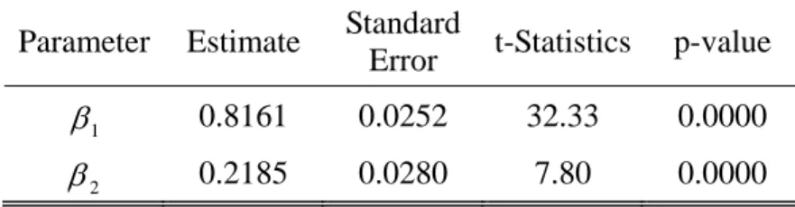
The stepwise regression chooses qw_t₋₁ and r_t₋₁ as the independent variables. Unemployment rates have little power in explaining the variation of surrender rates. The

regression results show that surrender rate increases with the surrender rate and interest rate

in the previous one period. Table 6 contains relevant estimation statistics.

Table 6: Estimated Parameters of the Surrender Rate Model

Parameter Estimate Standard

Error t-Statistics p-value

1

β 0.8161 0.0252 32.33 0.0000

2

β 0.2185 0.0280 7.80 0.0000

Correlation of Estimated Parameters: -0.00069 Intercept term is insignificant with p-value 0.8910.

2. Simulation of Surrender Rates and L

10

Strictly speaking, we should establish a surrender rate model for each type of policies since the surrender behaviors of different insurance may respond differently to unemployment rate and interest rate. We are unable to do so due to the lack of the data, however.

11

Since unemployment rates are reported monthly in the database, we use the average of monthly rates as the unemployment rate in that year. The one-year Treasury bill rates are also recorded monthly, we transform monthly interest rate to annual rate by the following compounding method:

annual interest rate = ) 1

12 m 1 )...( 12 m 1 )( 12 m 1 ( ₊ 1 ₊ 2 ₊ 12 ₋ _,

(20)

Using the above simple regression model and the 10,000 interest rate paths from

Section IV 3, we simulate 10,000 surrender rate paths with the mean of the sampled surrender

rate as the initial surrender rate.12 These surrender rates are then combined with simulated

mortality rates in Section III to determine the number of survivors as well as deaths in each

policy year and the corresponding cash flows. Combining the resulting 10,000 cash flow

paths with the 10,000 interest rate paths, we obtain the distribution of L under the

consideration of random mortality rates, stochastic interest rate, random parameters of the

interest rate model, and interest-rate-sensitive surrender rate. The simulation results are in

Table 7.

Table 7: Surrender Rate Risk (LR) + ETS + IR + MR

Confidence Interval Width of VaR Endowment -461,184 2,830,127 1.3170 2.3918 5,084,695 490,631 Pure Endowment -973,346 2,976,969 1.4240 2.7820 4,879,183 544,607 Term Life -192,551 856,483 0.9072 1.1395 1,444,830 113,158 Whole Life -324,687 4,538,632 3.2996 16.6294 7,966,843 1,100,364 Annuity 45,394 4,518,288 2.3492 8.3472 8,948,829 1,005,501

The right to surrender dramatically changes the reserve distribution. It makes the

12

We use the word ‘simulate’ instead of ‘obtain’ because we do not simply plug numbers into the regression model and calculate surrender rates directly. Instead, we simulate a random error from the error distribution of the regression first and then plug it into the regression model to generate a surrender rate.

(21)

distribution narrower as we can tell from the higher kurtosis (e.g., 2.39 vs. 0.95 for

endowment policy) and lower standard deviation (e.g., $2.8 million vs. $7.3 million for

endowment). The distribution is more positively skewed (e.g., 1.32 vs. 0.87) and its mean

shifts leftwards from $1 million to $-0.46 million in the case of endowment.

More importantly, the VaRs decrease significantly, which implies that the right to

surrender benefits the insurance company. An obvious reason for such decreases is the

surrender charge that is almost 20% for the first year and gradually descends with the policy

period. Since the insurer does not have to pay full amount of reserves to the policyholders

who surrender the policies, its liabilities decrease.

The drops of the VaRs are also due to the surrenders that happen during the periods of

low interest rates. Without surrenders, the insurer bears the entire adverse consequence of

low interest rates; with surrenders, the insurer suffers less because some policyholders

voluntarily terminate their polices during low interest rate era and such termination releases

the insurer from the 6% credit rate guarantee offered at the policy inception. In other words,

policyholders who choose to surrender their policies when interest rates are low indeed

relinquish a valuable guarantee offered by the insurance company and hence benefit the

insurer. This seemingly irrational behavior of surrender does exist in the history. For

instance, during the early 1960s, one-year rates are very low but surrender rates are still

(22)

ten percent of policies surrendered in 1997, 1998 and 1999.13 Our explanation for such

surrender behavior is that policyholders might keep or surrender their policies for reasons

other than the returns on insurance policies, e.g., changed demand. If return is not the only

reason for the policyholder to purchase a life insurance policy, the surrender behavior would

not solely depend on interest rate level. We thus would observe surrenders incurred in the

periods of low interest rate. The insurance company, on the other hand, always benefits

from the surrenders happening in low interest rate periods no matter which reasons the

policyholder surrenders for. Therefore, surrenders could reduce VaR and moderate interest

rate risk.

We can also explain the reduction in VaR due to surrenders by the concept of

incremental VaR discussed in Jorion (2001, p. 155 - 159). Incremental VaR, defined as the

change in VaR due to a new position, would be negative if the return of asset i is negatively

correlated with that of portfolio. We may consider our reserve VaR as a portfolio VaR with

respect to three fundamental risk factors: mortality rate, interest rate, and surrender rate.

When we consider only mortality rate risk, the positions in the other two risk factors are

assumed to be zero. The marginal impact of an additional risk factor is then similar to

incremental VaR. Hence, the marginal impact of a new risk factor could be negative if the

effects of risk factors are negatively correlated. Since low interest rates are harmful to

13

The number is estimated with the data from the Life Insurance Business in Japan (http://www.seiho.or.jp/english/index.html).

(23)

insurers but surrenders during these times are beneficial, they have opposite effects. The

marginal impact of surrender rate risk could be negative therefore, as long as the benefits

resulting from surrenders outweigh the harms. Furthermore, the negative effect of

surrenders on VaR is consistent with the findings about the decreased effective duration of

reserves resulting from surrenders documented in Babbel (1995), Briys and Varenne (1997),

and Santomero and Babbel (1997).

3. Parameter Estimation Risk of the Surrender Rate Model

To estimate the parameter estimation risk of the surrender rate model, we first assume

that the parameters

(

βˆ1,βˆ2

)

have a bivariate normal distribution with expected values and covariance structure as shown in Table 6. We then draw 10,000 samples of

(

βˆ1,βˆ2

)

from this bivariate normal distribution. From these 10,000 sets of parameters and the 10,000

interest rate paths from Section IV 3, we simulate 10,000 surrender rate paths. We then use

the same methodology as the one in Section V 2 to generate the distribution of L. Such

distribution is constructed under relatively comprehensive consideration: random mortality

rates, stochastic interest rate, interest-rate-sensitive cash flows, and parameter estimation

risks for both the interest rate and surrender rate models. We believe that this distribution of

L could render us valuable information about the risks of insurance policies. The statistics

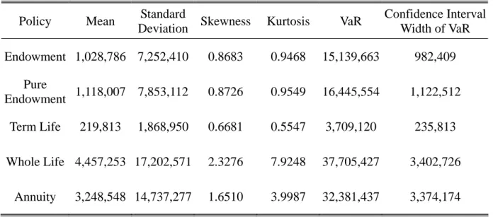
of the distribution are in Table 8.

(24)

Confidence Interval Width of VaR Endowment -651,380 2,540,448 0.8275 1.0945 4,070,062 299,554 Pure Endowment -1,195,002 2,580,961 0.8447 1.1730 3,565,619 323,476 Term Life -231,440 798,307 0.5839 0.4988 1,234,650 106,943 Whole Life -926,461 3,088,948 1.7815 6.0683 4,805,048 493,176 Annuity -446,892 3,568,499 1.3081 3.1089 6,308,442 606,786

The randomness of the parameters of the surrender rate model further decreases the

VaRs of insurance policies. Such decrease is reasonable because the randomness of

parameters enlarges the variations of surrender rate, results in more policyholders

surrendering their policies at the times of low interest rates, and thus leads to the VaR

decreases. The impact of the parameter uncertainty however is moderately significant only:

it makes merely ten percent changes in VaRs on average. The moderate significance comes

from the relatively small standard errors in Table 6.

Since the numbers in Table 8 are calculated by taking various relevant risks of

policies into consideration, they are reasonable estimates about reserves. They indicate that

the 95th percentile maximum shortfall of the reserve ranges from 0.5 to 2.3 times of annual

premiums for different types of policies, which is rather significant. Term life insurance is

(25)

insurance and annuity have the largest risk.14

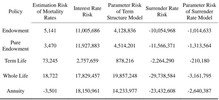
Table 9 displays the margin impact of risks on VaR. It shows that mortality rate risk

is unimportant, interest rate risk is the largest risk faced by insurers, and surrender rate serves

to alleviate interest rate risk. Furthermore, parameter estimation risks as derived risks

matter but are not as important as underlying risks. Our results suggest that insurers should

pay the most attention to interest rate risk, but should also be aware of the moderation effect

of surrender rate to avoid over-hedging.

Table 9: Marginal Impact of Risks on VaR

Policy Estimation Risk of Mortality Rates Interest Rate Risk Parameter Risk of Term Structure Model Surrender Rate Risk Parameter Risk of Surrender Rate Model Endowment 5,141 11,005,686 4,128,836 -10,054,968 -1,014,633 Pure Endowment 3,470 11,927,883 4,514,201 -11,566,371 -1,313,564 Term Life 73,245 2,757,659 878,216 -2,264,290 -210,180 Whole Life 18,722 17,829,457 19,857,248 -29,738,584 -3,161,795 Annuity -3,501 18,150,961 14,233,977 -23,432,608 -2,640,387

VI. Summaries and Conclusions

In this paper, we estimate the VaR of reserves for prevailing types of life insurance

14

The differences in risks among policies might even be larger if policies have different surrender tendency toward interest rate. More specifically, if annuity has more interest-rate-sensitive surrender rate than term life has, their VaRs will have larger differences than the one shown in Table 8 since the surrenders that are not sensitive to interest rate act to mitigate interest rate risk.

(26)

policies. To perform such estimation, we construct a simulation model featured with five

risk layers: the mortality rate risk from random mortality rates, the interest rate risk from

stochastic interest rate, the parameter estimation risk of the assumed interest rate model, the

early surrender risk from interest-rate-dependent surrender rate, and the parameter estimation

risk of the established surrender rate model. We also provide the confidence intervals of the

VaRs to check the accuracy of our estimation.

Consistent with the literature, our results show that the mortality risk is negligible but

the interest rate risk is substantial. We also find that the parameter estimation risk of the

interest rate model is noteworthy. The simulation further shows that the surrender option

may indeed benefit the insurance company: the emergence of early surrender reduces the VaR

of reserves. Probable explanations for such findings are the surrender charge and the

surrenders happening in low interest rate periods. The parameter uncertainty embedded in

the surrender rate model further augments the impacts of early surrender a little bit. The

above estimations are reasonably accurate, according to the widths of the confidence

intervals.

Several research topics might be worthy to be further pursued. First, other types of

mortality rate risk can be considered, e.g., the trend of decreasing mortality rates. Second,

future studies may want to assess the model risk of interest rate by trying alternative term

(27)

business) from our static analysis (closed-block business). Fourth, the asset/investment side

of business could be incorporated to generate surplus VaR that is the focal point of solvency

regulation and insurers’ risk management. The optimal asset allocation in terms of surplus

VaR given compositions of business would also be interesting.

References

American Council of Life Insurance, 1998, Life Insurance Fact Book (Washington D.C.:

American Council of Life Insurance).

Babbel, David. F., 1995, “Asset-liability matching in the life insurance industry,” in: Edward.

I. Altman and Irwin T. Vanderhoof, eds., The Financial Dynamics of the Insurance

Industry (New York: IRWIN Professional Publishing).

Beekman, John A. and Clinton P. Fuelling, 1990, “Interest and mortality randomness in some

annuities,” Insurance: Mathematics and Economics 9, 185-196.

Beekman, John A. and Clinton P. Fuelling, 1993, “One approach to dual randomness in life

insurance,” Scandinavian Actuarial Journal 2, 173-182.

Black, Kenneth, Jr. and Harold D. Skipper, Jr., 2000, Life and Health Insurance, 13th ed.

(Upper Salle River, New Jersey: Prentice Hall).

Bowers, Newton. L., Hans. U. Gerber, James C. Hickman, Donald A. Jones, and Cecil. J.

Nesbitt, 1986, Actuarial Mathematics (Schaumburg, Illinois: Society of Actuaries).

(28)

some common pitfalls,” Journal of Risk and Insurance 64, 673-694.

Cox, Samuel H., Paul D. Laporte, Steven R. Linney, and Lucian Lombardi, 1992,

“Single-premium deferred annuity persistency study,” Transactions of Society of

Actuaries Reports, 281-332.

Dowd, Kevin, 1998, Beyond Value at Risk: The New Science of Risk Management (New

York: John Wiley & Sons).

Duan, Jin-Chuan, 1994, “Maximum likelihood estimation using price data of the derivative

contract,” Mathematical Finance 4, 155-167.

Hogg, Robert V. and Elliot A. Tanis, 1997, Probability and Statistical Inference (Upper

Saddle River, New Jersey: Prentice-Hall International).

Jorion, Philippe, 2001, Value at Risk: The New Benchmark for Managing Financial Risk

(Taipei: McGraw-Hill).

Marceau, Etienne and Patrice Gaillardetz, 1999, “On life insurance reserves in a stochastic

mortality and interest rates environment,” Insurance: Mathematics and Economics 25,

261-280.

Outreville, J. Francois, 1990, “Whole-life insurance surrender rates and the emergency fund

hypothesis,” Insurance: Mathematics and Economics 9, 249-255.

Panning, William H., 1999, “The strategic uses of value at risk – long term capital

(29)

84-105.

Parker, Gary, 1994, “Moments of the present value of a portfolio of policies,” Scandinavian

Actuarial Journal 1, 53-67.

Parker, Gary, 1997, “Stochastic analysis of the interaction between investment and insurance

risks,” North American Actuarial Journal 1, 55-84.

Santomero, Anthony. M. and David F. Babbel, 1997, “Financial risk management by insurers:

An analysis of the process,” Journal of Risk and Insurance 64, 231-270.

Vasicek, Oldrich, 1977, “An equilibrium characterization of the term structure,” Journal of

Financial Economics 5, 177-188.