HE-AAC編碼器上之有效率的Time/Frequency Grid 設計

(1)

(2)

Efficient Design of Time/Frequency Grid in HE-AAC Encoder

Student Shou-Hung Tang

Advisor Chi-Min Liu

Wen-Chieh Lee

A Thesis

Submitted to Institute of Computer Science and Engineering College of Computer Science

National Chiao Tung University in partial Fulfillment of the Requirements

for the Degree of Master

in

Computer Science June 2006

(3)

SBR (Spectral Band Replication)

AAC MPEG-4 High Efficiency (HE) AAC

HE-AAC SBR AAC

SBR

(Time/Frequency

(4)

Efficient Design of Time/Frequency Grid in HE-AAC

Encoder

Institute of Computer Science and Information Engineering National ChiaoTung University

Spectral Band Replication (SBR) has been combined with MPEG AAC as bandwidth extension tool. The resulting scheme is referred to as the MPEG-4 High Efficient (HE) AAC or AACplus. With SBR module taking care of the high frequency contents, the conventional AAC encoder can compress the low frequency part using most of the available bits. From the similarity between the low and high bands, SBR reconstructs the high bands by replicating the low bands. In the SBR, the time-frequency (T/F) grids deciding the replication unit in high frequency bands are the kernel module in SBR. Frequency table decision, frame class decision, time segments and associated frequency resolution decision are the main design issues in T/F grid. The chosen frequency table and number of time segments determine the quality and consumed bits of reconstructed audio. Frame class restricts the number of time segments and the distribution of time borders. Therefore, the design of T/F grid should be greatly involved with quality and consumed bits.

This thesis proposes an approach that formulates the decision of the T/F grid into a trellis-lattice search problem and presents an efficient search algorithm to find the optimum path. Both subjective and objective tests are conducted to check the quality improvement over existing methods. The objective test measures used is the recommendation system by ITU-R Task Group 10/4.

(5)

(6)

Figure List

Figure 1: Components of HE-AAC and HE-AAC version 2...1

Figure 2: The basic principle of SBR for reconstructions. ...2

Figure 3: bit-rate quality comparison among AAC, HE-AAC, and HE-AAC version 2...2

Figure 4: Basic architecture of HE-AAC encoder. ...3

Figure 5: Block diagram of HE-AAC encoder. ...4

Figure 6: Block diagram of HE-AAC decoder [3]...7

Figure 7: Extracted parameters from bitstream mapping in HE-AAC decoder. ...8

Figure 8: Envelope estimation by interpolation mode and relating adjustment...9

Figure 9: Envelope estimation by non-interpolation mode and relating adjustment...10

Figure 10: Spectral valley from inappropriate range decision...12

Figure 11: Distortion for SBR range due to bad quality of AAC part. ...13

Figure 12: The spectral valley revising due to adaptive range adjustment..14

Figure 13: The parameters include in SBR header bitstream. ...15

Figure 14: The example for the characteristic of attack signal,...16

Figure 15 Time-direction dpcm disability...16

Figure 16: The range constraint of SBR [3]...16

Figure 17: Block diagram of 3GPP HE-AAC encoder [15]. ...18

Figure 18: The illustration of detection mechanism in transient detector....19

Figure 19: An example for T/F grid generator [15]. ...21

Figure 20: Illustration of DSR notation. ...27

Figure 21: The trellis-lattice deducing path by dynamic programming...27

Figure 22: DP flow chart with quality constraint...29

Figure 23: DP flow chart with both quality and efficiency constraint...30

Figure 24: An example for variable frame border...31

Figure 25: Tone trembling effect...32

Figure 26: An example for characteristics of tone-rich signals ...33

(9)

sharp...34

Figure 29: Sawtooth effect due to the limiter gain mechanism. ...35

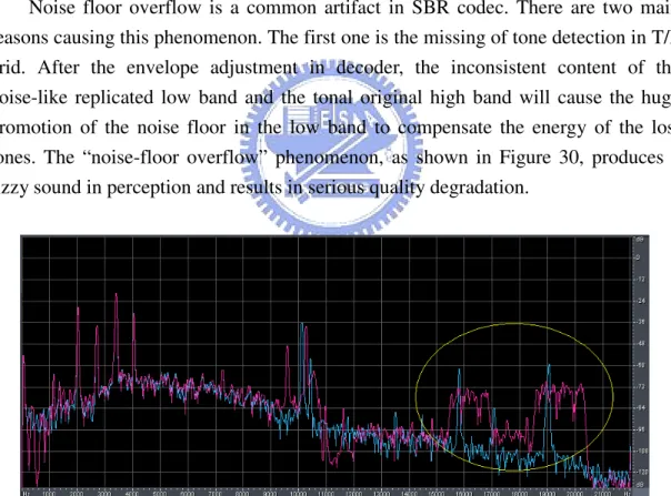
Figure 30: Noise floor overflow due to failure of detecting tones in high bands. ...35

Figure 31: Noise floor overflows due interpolation mode. The target circle indicates the noise floor overflow is from the averaged energy with tone component...36

Figure 32: A comparison to Figure 31. It incident the result without tone addition mechanism. ...37

Figure 33: The ODG variance comparison of Table 4...41

Figure 38: ODG-bit rate curve comparison among different T/F grid design. ...45

Figure 39: The average ODG of three coding methods in PSPLAB audio database at bit rate 80kbps and sampling rate 44100 Hz. M1 is uniform 1 cut in T/F grid and M2 is uniform 7 cuts in T/F grid. M3 is our design. ...47

Figure 42: The example for signal whose high band envelope alters rapidly. ...49

Figure 43: The example for signal which has a sharp high band envelope. 50 Figure 44: The error of noise floor due to tone addition...50

Figure 45: The spectrum of “sweep” which has continuous tone from 10 KHz to 22 KHz. ...51

Figure 46: The reconstructed spectrum of Figure 45 through uniform 7 cuts in T/F grid. ...51

Figure 47: The reconstructed spectrum of Figure 45 through DP T/F gird design. ...52

(10)

Figure 48: The reconstructed spectrum of Figure 45 through aacPlus. ...52

Figure 49: The spectrum of “sin_300_625_1k_5k_10k_15K_20k_m20db” which has interrupted tone from low frequency bands to high frequency bands ...53

Figure 50: The reconstructed spectrum of Figure 49 through DP T/F gird design. ...53

Figure 51: The reconstructed spectrum of Figure 49 through aacPlus. ...54

Figure 52: The frequency envelope of “sin_9kind_valious”. ...54

Figure 53: Noise floor overflow due to interpolation mode. ...55

Figure 54: The result of subjective test at 80 kbps. ...55

Figure 55: The ODG-bit rate comparison curve among different codecs....58

Figure 56: The result of objective quality measurement for error concealment based on MPEG test tracks at bit rate 80 kbps. ...59

Figure 59: The ODG and bit rate comparison curve for NCTU HE-AAC with and without error concealment. ...61

Figure 60: The frequency envelope of “sc01” by NCTU HE-AAC without error concealment...61

Figure 61: The frequency envelope of “sc01” by NCTU HE-AAC with error concealment. The blue line represents the original signal, and the red one is coded signal...62

(11)

Table List

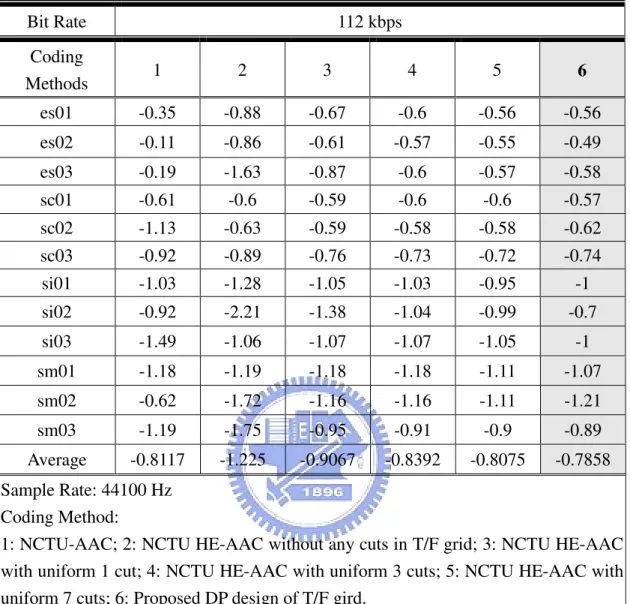
Table 1: The combination of transient and trailing frame borders...20 Table 2: Combinations of bit-consuming stages...29 Table 3: The twelve tracks recommended by MPEG ...39 Table 4: Objective measurements through ODGs for different T/F grid

design in HE-AAC at 112 kbps...40 Table 5: Objective measurements through ODGs for different T/F grid

design in HE-AAC at 96 kbps. ...41 Table 6: Objective measurements through ODGs for different T/F grid

design in HE-AAC at 48 kbps. ...44 Table 9: The PSPLAB audio database. ...46 Table 10: The objective quality measurement among different codecs at bit

rate 80 kbps...57 Table 11: The objective quality measurement among different codecs at bit

rate 64 kbps...57 Table 12: The objective quality measurement among different codecs at bit

(12)

Chapter 1 Introduction

Perceptual audio codecs (MPEG I Layer3 [1] or MPEG-II AAC [2] ) which exploit the properties of human psychoacoustic model not only reduce the transmitted audio data through eliminating the unheard frequencies and tones, but also provide “CD-quality” or “transparent” audio quality (indistinguishable source from encoded one) at a bit rate of 128kbps. Below 128kbps, the perceived audio quality of most codecs collapses rapidly. Due to insufficient bits, the codecs usually have two possible solutions that are the audio bandwidth limited or keeping the complete bandwidth but introducing annoying coding artifacts. The first solution makes the audio dull and the other results in unacceptable artifacts.

SBR (Spectral Band Replication) [3][4][5][6][7] which is standardized in ISO/IEC 14496-3:2001/Amd.1:2003 is a new audio coding enhancement tool and a significant breakthrough in the area of audio coding for low bit rates. SBR is a bandwidth extension tool used in combination with conventional audio codecs, e.g.

AAC (called aacPlus or HE-AAC), and MP3 (called mp3PRO [8]). Figure 1

demonstrates the components of HE-AAC and HE-AAC version 2. In addition to AAC and SBR codec, HE-AAC version 2 extra contains PS (Parameter Stereo) coding [9][10]. AAC SBR PS HE-AAC V1 HE-AAC V2 AAC SBR PS HE-AAC V1 HE-AAC V2

Figure 1: Components of HE-AAC and HE-AAC version 2.

The basic principle of SBR is to reconstruct the high frequency bands by replicating the low frequency bands and adjusting the replicated bands perceptually similar to original ones. The reconstruction procedure of SBR is illustrated in Figure 2.

(13)

encoder can compress the low frequency part with most of the available bits. Hence, SBR not only can increase the audio bandwidth, but improve the quality of underlying codec at low bit rates. The bit rate-quality comparison among AAC, HE-AAC version 1 and HE-AAC version 2 is illustrated in Figure 3. AAC has good performance at the bit rate over 96K, HE-AAC (SBR) targets at the range from 48K to 80K, and HE-AAC version 2 (PS) is responsible for the bit rate lower than 48K.

Original Signal

SBR Reconstruction Process

Original Signal

SBR Reconstruction Process

Figure 2: The basic principle of SBR for reconstructions.

0 32 64 96 128 0 20 40 60 80 100 Q ua lit y Excellent Poor Fair Good

Stereo bit-rate [kbit/sec] Bad HE-AAC+PS AAC HE-AAC B an dw id th Channels 0 2 fs/2 AAC fs/4 AAC SBR AAC SBR PS 1 0 32 64 96 128 0 20 40 60 80 100 Q ua lit y Excellent Poor Fair Good

Stereo bit-rate [kbit/sec] Bad HE-AAC+PS HE-AAC+PS AAC HE-AAC B an dw id th Channels 0 2 fs/2 AAC AAC fs/4 AAC SBR fs/4 AAC SBR AAC SBR AAC SBR PS 1

Figure 3: bit-rate quality comparison among AAC, HE-AAC, and HE-AAC version 2. SBR is an advanced scheme to compress high frequency contents efficiently at very low bit rate, commonly about 1K~3K bps per channel [5]. Under bit rate constraint, the existing audio codecs sacrifice the high frequency component of

(14)

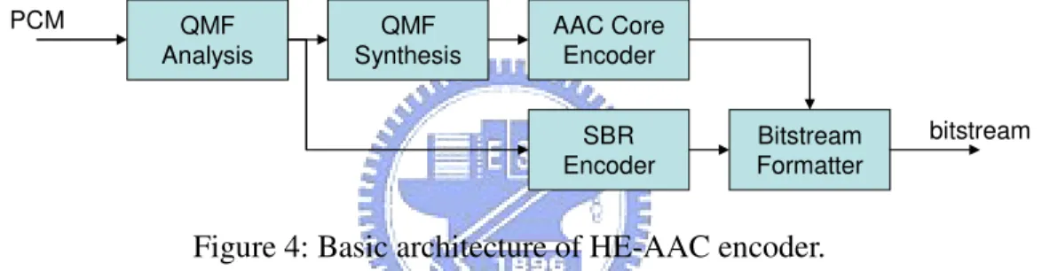
signals to obtain good perceptual quality. However, when the audio bandwidth is getting lower, the hearing perception becomes duller. SBR is responsible for retaining the signal bandwidth at low bit rate. Through SBR taking care of the high frequency parts of the audio signals with small amount of bits, the conventional encoder only needs to handle the low frequency parts. Consequently, the signal fed into underlying encoder half of the original sample rate is enough based on Nyquist’s theorem. Inherently, HE-AAC is a dual rate system, where the AAC encoder is operated at half the sampling rate of SBR encoder. The basic architecture of HE-AAC encoder is depicted in Figure 4. The audio signal is fed into the 64-bands Analysis Filter. After the Analysis Filter, there are two branches where one is SBR encoder and the other is 32-bands Synthesis Filter. Through 64-bands Analysis Filter and 32-bands Synthesis Filter, the signal fed into AAC encoder is half the sampling rate of the original signal.

QMF

Analysis SynthesisQMF AAC CoreEncoder SBR

Encoder FormatterBitstream PCM

bitstream

Figure 4: Basic architecture of HE-AAC encoder.

In the SBR encoder, the control parameters is estimated to ensure that the reconstructed high frequency bands are as similar as original ones. These parameters mostly for spectral envelope representation are used to rescale the spectral envelope and control the tonal-to-noise ratio of high frequency bands. Time-frequency (T/F) grid and High frequency (HF) generator are the two main modules in SBR codec. The former decides the reconstruction unit in time and frequency domains for rescaling the replicated envelopes to original ones, and the latter keeps the similarity of noise-to-tone ratio between replicated contents and original ones. The resolutions of reconstruction units dominate the accuracy of the reconstructed contents and required bits. The higher is resolution of these units; the better is the accuracy of reconstruction, but taking more bits. Hence, T/F grid plays a key role to determine the resolutions of reconstruction units and dominates the resulting audio quality of whole HE-AAC.

The block diagram of SBR encoder is illustrated in Figure 5. In SBR encoder, the SBR range is determined in the first. Frequency table decision is responsible for choosing the most suitable frequency resolution from eight different tables. Tonality calculation estimates the tonality of original signal. T/F grid determines the number of time envelopes, time borders, and envelope resolutions. According to the information

(15)

ratio, additional tone and noise is established by Tone/Noise Addition module. Finally, through quantization and delta coding eliminating redundancy between encoded data, the information from SBR encoder and AAC encoder is combined into bitstream packet. The Coupling module determines that stereo or coupled to mono compressing in SBR encoder. The Bit Reservoir module plays the role of allotting bits among SBR encoder and AAC encoder. The shadowed modules are the main topics in this thesis, including SBR range decision, frequency table decision and Time/Frequency grid.

! "" ! "" # $ # $ Input Signal Coded Audio Stream % % & & ! "" ! "" # $ # $_$# # $_$# # $ Input Signal Coded Audio Stream % % & &

Figure 5: Block diagram of HE-AAC encoder.

Since HE-AAC comprises SBR and AAC, the cooperation among them is very important. The reconstructed high frequency bands by SBR depend on replicated low

(16)

frequency bands, and therefore, the quality of AAC encoder has significant effect on HE-AAC. The SBR range and associated AAC range decision is the first important design issue in HE-AAC encoder. With inappropriate allocation for AAC and SBR range, it may bring the artifact “spectral valley” around range boundary or reduce the quality of HE-AAC encoder. The range decision is involved with contents of signal, compressing bit rate and sampling rate. In existing SBR encoder, including 3GPP [11], Coding Technology [12] and Nero [13], the SBR range is determined only by bit rate and sampling rate. This thesis proposes a method to determine the most appropriate SBR range taking account of above factors.

The resolution of reconstruction unit used in SBR process is determined by Time/Frequency grid module. This module can be incised into three parts, which are frequency table decision, time borders distribution and associated envelope frequency resolution decision and frame class decision. Frequency tables describe the approximate resolution of reconstruction unit in frequency domain, and time borders revolve the resolution in time domain. Envelope resolution define the detailed frequency resolution each frame. There are four different SBR frame classes, FIXFIX, FIXVAR, VARFIX, and VARVAR used, each of which has different capabilities to describe the distribution of time borders. Appropriate frame classes selection can increase the coding efficiency. Bit rate, content of signal greatly affect T/F Grid decision. In 3GPP SBR encoder, it introduces a transient detector to detect the start position of transients and labeling time borders. It only considers energy difference of neighbor samples without the correlation between replicated samples and original ones. This thesis formulates the decision of the T/F grid into a trellis-lattice search problem and proposes an efficient search algorithm to find the optimum solution.

This thesis is organized as follows. Chapter 2 introduces the fundamental knowledge of HE-AAC. Chapter 3 introduces the design of SBR range cooperating with AAC encoder. In Chapter 4, the existing T/F grids designs are described. Chapter 5 presents an efficient design of T/F grids through dynamic programming. In Chapter 6, extensive experiments are made to prove the improvement of the proposed T/F grid design. Both subjective and objective measurements are conducted to verify the quality and efficiency of our T/F grids in Chapter 5. Chapter 7 gives a conclusion and future work on this thesis.

(17)

Chapter 2 Backgrounds

2.1 SBR Decoder Overview

The block diagram of HE-AAC SBR decoder [3] is illustrated in Figure 6. It shows the relationship between AAC decoder and SBR enhancement parts. First, the bitstream payload deformatter divides the bitstream payload into AAC parts and SBR parts. The AAC bitstream part is fed to the AAC decoder, and the SBR bitstream part is fed to the bitstream parser. After the parser, de-quantization follows and the raw data is Huffman decoded. Through an analysis QMF bank, the low frequency part of signal from AAC decoder separated into 32 subbands is fed into HF Generator which is responsible for deriving the high frequency part according to SBR data and the low frequency part of signal. Envelope Adjuster is guided by the SBR data extracted from the bitstream to adjust the reconstructed components as similar as original ones. Finally, the low frequency parts and the high frequency parts are synthesized by a synthesis QMF bank.

(18)

Coded Audio Stream Bitstream Payload Deformatter Bitstream Parser AAC Core Decoder Huffman Decoding & Dequantization Envelope Adjuster HF Generator Analysis QMF Bank Synthesis QMF Bank Output PCM Samples

Figure 6: Block diagram of HE-AAC decoder [3].

2.2 HF Generator

In the HF generator, the goal is to copy or patch a number of low frequency subband signals obtained from the analysis filter bank to consecutive high frequency subband signals. The patching determines the corresponding relation between high bands and replicated low bands. In addition, in order to remove the unwanted tone components, the inverse filtering is done in this module. Hence, the output of HF generator is the corresponding subband signal for reconstructing original high frequency subband.

2.3 Envelope Adjuster

The objective of envelope adjuster is to adjust the reconstructed envelop as similar as original one. The envelope adjustment is accomplished according to the parameters extracted from bitstream. With the original high band energies and additional components for each reconstruction unit from bitstream, the corresponding

(19)

2.3.1 Parameter Mapping

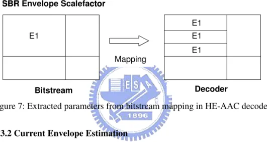
Some of the parameters extracted from the bitstream are vectors or matrices. Out of necessity, this grouped data is mapped to the highest available frequency resolution for the envelope adjustment. This means that the adjacent subbands in the grouped data will have the same value. However, the mapping is only in the frequency domain, and time resolution will be preserved. Figure 7 shows the mapping of envelope scalefactor. Bitstream SBR Envelope Scalefactor Mapping E1 E1 E1 E1 Decoder Bitstream SBR Envelope Scalefactor Mapping E1 E1 E1 E1 Decoder

Figure 7: Extracted parameters from bitstream mapping in HE-AAC decoder.

2.3.2 Current Envelope Estimation

In order to adjust the envelope of the present SBR frame, the envelope of the current SBR signal needs to be estimated. There are two different estimation mode used in SBR codec, interpolation and non-interpolation. With interpolation, the estimated current envelop_{E is given by}'

( )

(

)

( )

(

1

)

,0 1,0 1 2 , , 1 1 2 2 2 ' _≤ _≤ ₋ _≤ _≤ ₋ − − ⋅ + = − + ⋅ ⋅ = E E E l t l t i h x L l M m l t l t i k m X l m E E E (1)

The notations are illustrated below

m : QMF subband index

l: Time envelope index

x

k : the first QMF subband in the SBR range. (SBR start boundary)

E

t : contains the time borders for all SBR envelopes in the current SBR frame.

M: The total amount of QMF subband in SBR range.

E

L : Number of SBR envelopes.

If non-interpolation is used, the energies are averaged over every frequency band. The estimation is

(20)

( )

(

)

(

)

( )

(

) (

)

( )

(

)

( )

(

1,

)

1,0

( )

1 , , , 1 1 2 , , ), , ( , 1 1 2 2 2 ' ' ' − ≤ ≤ − + = = ≤ ≤ − − ⋅ − + ⋅ = − − = − + ⋅ ⋅ = = l r n p l r p F k l r p F k k m k k k l t l t i j X l k k E l k k E Mapping l m E h l h l l h E E l t l t i k k j h l h l h E E h l (2)

( )

l r : Envelope resolution

( )

r l

n : Number of frequency band

( )

F : Frequency band table

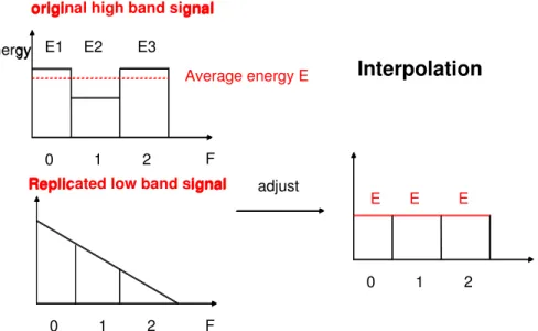
The difference between interpolation mode and non-interpolation mode is illustrated in Figure 8 and Figure 9. In interpolation mode, the energies are averaged over every QMF filter band, and each QMF subband derives respective gain value. All the OMF subbands in one frequency band will be adjusted to the same energy. In non-interpolation mode, the energies are averaged over every frequency band. All the QMF subbands in one frequency band use the same gain value, and the envelope of replicated signal will be maintained.

F 0 1 2 energy 0 1 2 E E E 0 1 2 E1 E2 E3 adjust

original high band signal

Replicated low band signal

F

Average energy E Interpolation

F

(21)

F

Figure 9: Envelope estimation by non-interpolation mode and relating adjustment

2.3.3 Additional HF Components and Gain Calculation

The noise floor scalefactor is a ratio, and in order to add the correct amount of noise, it needs to be converted to a proper amplitude value, according to the following.

( )

( ) ( )

_{( )}

,0 1,0 1 , 1 , , , ≤ ≤ − ≤ ≤ − + = m M l L_E l m Q l m Q l m E l m Q (3)

The level of sinusoids are derived as

( )

( ) ( )

_{( )}

l m Q l m S l m E l m S , 1 , , , + = (4)

And the gain value are derived by

( )

(

( )

)

( )

⋅ +

( )

≠ = + ⋅ = 0 , , , 1 , , , 0 , , , 1 , , , ' ' l m S if l m Q l m Q l m E l m E l m S if l m Q l m E l m E l m G (5)

In order to avoid unwanted noise substitution, the gain values are limited according to the limiter gain mechanism:

(22)

( )

( ) ( )

( )

( ) ( )

( )

(

)

( )

(

1

)

, 1 0 , 10 , _ lim _ limGain , , min ) , ( , lim lim 5 ' 1 1 1 1 lim lim lim lim + ≤ ≤ − ≤ ≤ ⋅ = = − + = − + = k f m k f N k gains iter bs l i E l i E l k G Mapping l m G L k f k f i k f k f i Max Max (6)

where_limGain₌

[

₀_.₇₀₇₉₅_,_1.0,_1.41254,₁₀10

]

_{, and} lim

f presents the limiter frequency

band. Hence, the gain values are limited according to

( )

m l

(

G

( )

m l G

( )

m l

)

G_lim , =min , , _Max , (7)

The additional noise component needs to be revised by

( ) ( )

m l Q m l G_G

_{( )}

_m

( )

m_ll Q , , , , lim lim = ⋅ (8) Due to the limitation, the total energy for a limiter band will have loss, and it is compensated by

( )

(

( )

)

( )

( ) ( )

( )

(

)

( )

( ) ( )

( )

(

)

( )

≠ + = + = = − + = − + = − + = − + = 584893192 . 1 , 0 , , , * , , 0 , , , * , , min , , 1 1 ) ( 2 2 lim 1 1 1 1 ) ( 2 lim 2 lim 1 1 lim lim lim lim lim lim lim lim l m S if l i S G l i E l i E l m S if l i Q G l i E l i E l k G Mapping l m G k f k f i k f k f i k f k f i k f k f i C C (9)

Finally, the resulting gain values and additional components are

( )

( ) ( )

m l S m l G

( )

m l S l m G l m Q l m Q l m G l m G l m G C final C final C final , , , , , , , , , , , lim lim ⋅ = ⋅ = ⋅ = (10) HF Signal Assembling

Before the gain values are applied to the subband samples, there is a filter to smooth the gain values. The smooth filter is applied according to the parameters extracted from bitstream. Finally, the subband samples are adjusted by these gain values, and the additional noise and tone components are added.

(23)

Chapter 3 SBR Range Decision

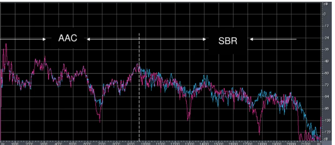
SBR range decision here is to decide a boundary in frequency domain. This boundary separates QMF data into two portions. Frequency bands lower than the boundary is to be coded by AAC encoder, and frequency bands higher than the boundary is to be coded by SBR encoder. SBR replicates the subband signals encoded by AAC to reconstruct high frequency subband signals. Therefore, the quality of SBR encoder greatly relies on AAC encoder. In other words, the objective of SBR range decision is to ensure that the low frequency parts encoded by AAC can have a satisfactory quality. The range decision allots the burdens between SBR encoder and AAC encoder, which is a decided module for HE-AAC quality. With inappropriate range disposing, it may bring perceptible artifacts therefore reduce the audio quality. While selected SBR start frequency is too high, available bits may not be enough for AAC to encode the assigned bandwidth. HE-AAC may produce “spectral valley” around range boundary due to insufficient bits. Figure 10 illustrates an example of resultant spectrum with spectral valley. The quality of low frequency components also influences the high frequency components reconstructed by SBR. Figure 11 shows an example of distortion in high frequency due to bad quality of low frequency component. Oppositely, if bits are sufficient and the bandwidth assigned to AAC is too narrow, since the maximum bandwidth of SBR is restricted, the overall bandwidth of HE-AAC is getting lower and decreases the audio quality. Obviously, bit rates and sampling rates are the main factors to this range decision.

AAC SBR

(24)

AAC _SBR

Figure 11: Distortion for SBR range due to bad quality of AAC part.

Another significant factor to SBR range decision is the contents of signal. The required bits of AAC encoder are related to the audio content. Thus, whether or not the available bits are sufficient is related to signal contents. Even at high bit rates, the spectral valley still occurs in the trailing of AAC parts because the relating audio content is hard to be encoded. On the contrary, at the low bit rates, the bandwidth of AAC is not necessary to be cut off.

Therefore, SBR range decision is greatly involved with bit rates and audio content. The consideration of audio content is aggressive and active, and the consideration of bit rates is steady and conservative. According to the two factors, this thesis proposes two possible approaches, which are adaptive SBR range and error concealment.

3.1 Adaptive SBR Range Adjustment

The required bits for each frame in AAC encoder are different due to the contents of signal. Consequently, the most flexible method is adaptively adjusting SBR range according to condition of AAC encoder. Through detecting the zero bands in AAC bit allocation, SBR range can be determined adaptively frame by frame. The adaptive method not only eliminates the spectral valley artifact, but achieves good interconnection between AAC encoder and SBR encoder. Giving Figure 6 for an example, there are zero bands in the trailing of AAC parts. By detecting these zero bands, the SBR range can move ahead to avoid the spectral valley. Figure 12 shows the result.

(25)

AAC SBR

Figure 12: The spectral valley revising due to adaptive range adjustment. However, this method may face four shortcomings: the SBR header overhead, tone trembling artifact, reduced efficiency for the DPCM and the fluctuated bandwidth.

3.1.1 SBR Header Overhead

SBR encoder uses several different frequency band tables, which are master band frequency table, high resolution frequency band table, low resolution frequency band table, noise floor frequency band table and limiter frequency band table. The parameters in SBR bitstream header are needed to define all frequency band tables, SBR start boundary and stop boundary. If the bitstream parameters used for this frame are the same as the last one, then the bitstream header needs not to be transmitted again. On the contrary, a transmission of the header is only needed when the parameters differ from the last ones. Therefore, adaptively revising SBR range needs to consume bits for transmitting new bitstream header. The syntax of SBR header is illustrated in Figure 13. In SBR header, the two parameters bs_start_freq and bs_stop_freq define the SBR range. According to Figure 13, the overhead for varying bs_start_freq and bs_stop_freq is 16bits. Therefore, altering SBR range each time

(26)

SBR Bitstream Header bs _a m p_ re s 1 bs _s ta rt _f re q 4 bs _s to p_ fr eq 4 bs _x ov er _b an d 3 bs _r es er ve d 2 bs _h ea de r_ ex tr a_ 1 1 bs _h ea de r_ ex tr a_ 2 1 bs _f re q_ sc al e 2 bs _a lte r_ sc al e 1 bs _n oi se _b an ds 2 bs _l im ite r_ ba nd s 2 bs _l im ite r_ ga in s 2 bs _i nt er po l_ fr eq 1 bs _s m oo th in g_ m od e 1 SBR Bitstream Header bs _a m p_ re s 1 bs _s ta rt _f re q 4 bs _s to p_ fr eq 4 bs _x ov er _b an d 3 bs _r es er ve d 2 bs _h ea de r_ ex tr a_ 1 1 bs _h ea de r_ ex tr a_ 2 1 bs _f re q_ sc al e 2 bs _a lte r_ sc al e 1 bs _n oi se _b an ds 2 bs _l im ite r_ ba nd s 2 bs _l im ite r_ ga in s 2 bs _i nt er po l_ fr eq 1 bs _s m oo th in g_ m od e 1

Figure 13: The parameters include in SBR header bitstream.

3.1.2 Tone Trembling

Tone trembling is an artifact which greatly decreases the audio quality in the perceptual hearing. The characterization of this artifact will be described in Chapter 6.

3.1.3 Reduced Efficiency of DPCM

A single sinusoid in the frequency domain transforms to a stable signal in the time domain, and on the contrary, a pulse in the time domain corresponds to a constant in the frequency domain. Figure 14 describes the above property of audio signal. On a word, most signal is usually stable in either time or frequency domain. Therefore, using delta coding in one of these two domains according to the signal characteristics can increase the coding efficiency. In Figure 15, since the SBR range of this frame differs from the last one, the number of subband included in SBR range is different between two consecutive frames. It disables time-direction DPCM for the first envelope of this frame. Consequently, the incomplete DPCM takes more bits and decreases the coding efficiency.

(27)

Figure 14: The example for the characteristic of attack signal, AAC AAC T F DPCM AAC AAC T F DPCM

Figure 15 Time-direction dpcm disability

3.1.4 Fluctuated Signal Bandwidth

The subband number of SBR range is restricted by standard in Figure 16. According to different sampling rate, the different maximum ranges are defined. Since the SBR start boundary is adjusted adaptively, in order to observe this restriction, the stop boundary may need to be moved ahead. Consequently, the bandwidth of signal may vary with frames. In addition, the changing of SBR stop boundary may also cause tone trembling artifact. Regardless of tone trembling, the fluctuated bandwidth makes signal intermittent and reduce the audio quality in perceptual hearing.

2 0

48 ,

32 35 ,

44.1 32 ,

48

SBR SBR SBR

Fs

kHz

k

Fs

kHz

Fs

kHz

≤

− ≤

=

≥

Figure 16: The range constraint of SBR [3].

(28)

Integrating the above discussion, the adaptive SBR range method will face many difficulties. The most serious problem is the bit overhead. In order to record the change of range, more bits are used for transmitting bit stream. Hence, this method has the highest flexibility but loses the coding efficiency. However, SBR is used for low bit rate coding. Instead of high coding precision, SBR turns to economize required bits for acceptable reconstructed signal. Therefore, at low bit rates, the adaptive range approach seems unsuitable.

3.2 Error Concealment

This method determines SBR range depending on bit rates and sampling rates. The SBR range is fixed among frames. According to bit rates, the burden allocation between AAC encoder and SBR encoder is fine in most frames. The occasional spectral distortion is handled by error concealment mechanism [14][15][16][17] in SBR decoder. This approach leads high coding efficiency, and error concealment mechanism can compensate the lack of flexibility. Further, due to the help or error concealment, the bandwidth of reconstructed signal can be aggressively extended.

(29)

Chapter 4 Related Work for Time/Frequency

Grid

This chapter introduces the design of T/F grid in 3GPP HE-AAC encoder [15]. The block diagram of 3GPP HE-AAC encoder is illustrated in Figure 17. T/F grid decision contains transient detector, frame splitter, and T/F grid generator. Transient detector detects the start position of transient. Frame splitter is only operated in the frame without transient, and it determines this frame separated into two envelopes or not. T/F grid generator receives the information from transient detector and determines the time borders and the related envelope resolution.

64 c h A na ly si s Q M F Transient detector Frame splitter PCM signal (L/R/M) _Tonality detector T / F Grid Generator Additional Control Parameters Envelope Energy Formatter Quantiser and T/F Huffman Encoder B its tr ea m M ul tip le xe r Coded SBR Bitstream

Figure 17: Block diagram of 3GPP HE-AAC encoder [15].

4.1 Time/Frequency Grid Design

In 3GPP SBR encoder, the frequency band table is selected depending on bit rate and sampling rate and it does not alter among frames. Time segments, envelops

(30)

resolution and frame classes are determined according to below mechanism. 4.1.1 Transient Detector

Transient detector is the most important module in 3GPP T/F grid. The following frame splitter and T/F grid generator operates according to the information from it. On a word, the SBR coding quality relies on this module.

The objective of transient detector is to determine whether a transient occurs in the present frame and find the position for the on-set of the transient. The output variables of transient detector, tranFlag and tranPos are used for recording the above information.

Transient detector operates on subband samples of one frame length and starts from sample 8. The basic principle of transient detector is to estimate the energy difference among samples, and determines whether a transient exists depending on information of energy difference. At first, calculate the average energy of each subband in the processed frame and then derive the standard deviations. Next, for each subband, calculate the neighbor energy difference of each sample and compare it to the relating standard deviations. If the energy difference is larger then the relating standard deviations, then take down the value which exceeds the standard deviation. For each time samples, the estimation procedure is executed 64 times, and the values indicating “large energy difference” are added. Finally, check each sample whether one with the energy difference value exceeds the threshold. If it does, then set tranFlag to true, and record the position of this sample. The diagram of transient detector is illustrated in Figure 18. Time samples QMF Subbands d1 d2 d3 1 2 64 E1 E2 E3 E4 E32 63 Energy Difference d4 d32 Time samples QMF Subbands d1 d2 d3 1 2 64 E1 E2 E3 E4 E32 63 Energy Difference d4 d32

(31)

4.1.2 Frame Splitter

Frame Splitter only operates when transient detector has detected the absence of a transient in the current frame. It decides whether the current frame is split into two envelopes of equal size and uses a variable splitFlag to store the result. The concept of frame splitter similar to transient detector is to estimate the energy difference, but not as precise as transient detector. The estimation unit used in this module is half of frame length. Compare the energies of the two half frame, the variable splitFlag can be determined.

4.1.3 T/F Grid Generator

The T/F grid generator creates the time/frequency grid for one SBR frame. Input parameters are provided by transient detector and frame splitter. Frame class is determined at first. It is accomplished depending on the trailing frame border of last frame (FIX or VAR) and the parameter tranFlag of the present frame. On a word, if there is a transient in the current frame, the trailing frame border is VAR; else, the trailing frame border is FIX. The total combination of the leading frame border and transient is described in Table 1. When most transients are sparse, the FIXVAR-VARFIX pair is used. The current frame is encoded with the FIXVAR portion, and the VARFIX gird is stored for the next frame. If no transient occurs in the next frame, the stored VARFIX grid is used; else, the new calculations are needed for the new transient, and merged with the already calculated grid, whereby, a VARVAR class frame is used.

VARVAR VARFIX VAR FIXVAR FIXFIX FIX 1 0 VARVAR VARFIX VAR FIXVAR FIXFIX FIX 1 0 Leading Frame Border TransFlag VARVAR VARFIX VAR FIXVAR FIXFIX FIX 1 0 VARVAR VARFIX VAR FIXVAR FIXFIX FIX 1 0 Leading Frame Border TransFlag

Table 1: The combination of transient and trailing frame borders.

The positions of time borders in one frame are determined mainly on the position of transient, i.e. the input parameter tranPos provided by transient detector. Each

(32)

transient accompanies three main time borders, the first one locates at the position for on-set of the transient, the second one is two timeslots behind the first border, and the third one is four timeslots after the second one. In addition, if the position of transient is not too near the front of the current frame, there will be additional time border ahead the transient. Similarly, additional time borders may be adopted behind the transient when the transient is in the front of the present frame. For Figure 19 as example, the tranPos is 13, and the resulting main time borders locate at 13, 15, and 19. The additional time borders are at 7 and 25 respectively. Consequently, the time borders in the present FIXVAR frame locate at 7, 13, 15, and trailing frame border is at 19. The grid contents of VARFIX portion will be stored for the next frame.

tranFlag = 1

tranPos = 13

|<- Frame n: FIXVAR-:--3->|< Frame n+1: -->|

... QMF slots

I-|-|-|-|-|-|-|-|-|-|-|-|-|-|-|-Io|o|o|-|-|-|-|-|-|-|-|-|-|-|-|-I SBR slots

0 7 13 15 19 25 32 FG index

I: nominal frame boundaries

o: frame overlap region slots

VARFIX

Figure 19: An example for T/F grid generator [15].

4.2 Summary

On a conclusion, the key in the 3GPP T/F grid is the transient detector. Time borders are greatly involved with the position for the on-set of the transient. If there is a transient detected in the present frame, regardless of additional time borders, it creates three time borders at least. The number of time borders can be considered as the required bits. Therefore, the objective of T/F grid is to use the least number of time borders to achieve satisfactory audio quality. In 3GPP T/F grid, some time borders can be removed to economize the consumed bit for the coding efficiency.

However, the most existing SBR encoder adopts the concept of transient detector, including Coding Technology [18] and US 2006/0031065 A1 [19], for T/F grid. Instead of detecting of position of transient, this thesis analyzes the design issues of

(33)

Chapter 5 Efficient Design of Time/Frequency

Grid

Time/Frequency Grid decides the format of reconstruction unit in both time and frequency domain. The resolution of reconstruction unit determines the accuracy degree of reconstructed signal and required bits. It is obvious that for stable signal, the format of T/F grid should be “simple” to reduce the required bits. Oppositely, in order to reduce the distortion of reconstructed signal, the format of T/F gird should be dedicated. In addition, if there are more available bits, the resolution of T/F grid can be higher. Consequently, T/F grid decision is greatly involved with bit rate and audio contents. The efficient design of T/F Grid which this thesis proposes emphasize on these two main factors.

The first issue is how to judge a T/F grid assignment is good or poor. This paper introduces a method to measure the reconstruction error of signal objectively. With the analysis of error, collocating different bit rates, the most suitable form of T/F grid can be selected.

T/F grid comprises frequency table decision, time borders distribution, envelope resolution decision and frame class decision. Frequency tables and envelope resolution codetermine the frequency resolution of T/F grid, and time borders distribution and frame class are responsible for time resolution. The reconstruction error measurement is described first, and the designs of other sub-modules are followed.

5.1 Analysis of Reconstructed Error

The process of SBR decoder has been described in Chapter 2. Through simulating the concept of reconstruction in decoder, the corresponding reconstructed error can be estimated. The reconstructed error used in this thesis is defined as error of power spectrum. The estimation process is accomplished as follows:

First, the rescaling gain values can be hypothesized to the power spectrum of original high frequency contents divided by corresponding low frequency ones. It is given by

(34)

∈ ∈ = g i ig g i ig g L H , , α (11)

Where H_i_,_g represents the power spectrum of high frequency band samples in one grid unit, and L_i_,_g stands for the corresponding power spectrum of low frequency band samples, i.e.

2 2 i i i i l L h H = = (12) Where theh is the high frequency band sample, and_i l is the related low frequency _i

band sample.

The number of grid units and related α is determined by the form of T/F grid, _g using G as notation. Consequently, the reconstructed envelope error of T/F grid is estimated by

( )

∈ ∈ − = G g i g ig g ig L H G E _, α _, 2 (13)

Next, the goal is to find one kind of T/F grid to minimizeE

( )

G , which can be expressed by

( )

[

E G

]

Arg G G min = (14)

And (13) is expressed as follows.

( )

− = + − = + − = − = ∈ ∈ ∈ ∈ ∈ ∈ ∈ ∈ ∈ ∈ ∈ ∈ ∈ ∈ G g gi g ig ig G g i g ig G g g i g ig G g gi g ig ig G g i g ig G g i g ig g ig ig g ig G g i g ig g ig H L H L H L H L H L H L H G E , , 2 , 2 , 2 , , 2 , 2 , 2 , , 2 , 2 , , 2 2 2 2 α α α α α α (15)

(35)

( )

[

]

= = ∈G ∈ g g i g ig ig G GArg E G Arg L H G min max α _, _, (16)

Furthermore, it can be expressed as follows

⋅ = ⋅ = ∈ ∈ ∈ ∈ ∈ ∈ ∈ ∈ ∈ ∈ ∈ g G g i ig g i ig g i ig ig g i ig G g i g ig ig g i ig g i ig G g gi g ig ig L H H L H H L L H H L , , , , 2 , , , , , , , * α (17)

It is clear to see that the error is related to the energy of original high frequency contents and the correlation between high frequency bands and replicated low frequency bands.

According to (17), the reconstructed error will be affected more by the high energy samples than small energy ones. Therefore, the T/F grid which is picked out through minimumE

( )

G tends to take care of samples with large energy, and may ignore the others with small energy. However, the distortion of small energy samples is huge, and makes the reconstructed signal sounds noisy. In order to overcome this problem, this paper introduces critical unit to revise the criterion. Critical unit is used for energy normalization and defined as follows, in the time domain, each critical unit contains four samples(two timeslots), and in the frequency domain, the resolution of critical unit is involved with critical band bandwidth, i.e. the critical unit contains fewer subbnads in low frequency and more subbands in high frequency. Instead of minimum error, the objective is the minimum distortion rate, and (13) is revised by

∈ ∈ ∈ − ∈ G c c i ic c i ic i c gi ic H L H 2 , 2 , ) ( , α (18)

Comparing (13) with (18), the measurement unit is magnified form sample to critical unit. In order to reduce the calculation complexity, (18) can be changed into a radical expression

(36)

∈ ∈ ∈ ∈ ∈ ∈ ∈ ∈ − = − G c c i ic c i ic i c g i ic G c c i ic c i ic i c gi ic H L H H L H , , ) ( , 2 , 2 , ) ( , α α (19)

The calculation of (19) is defined as DSR (energy difference to original signal ratio). Finally, the reconstructed error estimation is given by

( )

[

]

= − = ∈ ∈ ∈ ∈ G c c i ic c i ic i c g i ic G G H L H Arg G DSR Arg G , , ) ( , min α (20)

Due to the frame boundaries can be variable; the number of critical unit in each frame is different. Consequently, (20) is revised by

( )

[

]

− = = ∈ ∈ ∈ ∈ ∈ G c G c c i ic c i ic i c g i ic G G H L H Arg G DSR Arg G 1 min , , ) ( , α (21)

To summarize, the objective of T/F grid decision is to find a format of T/F grid to minimize the averaged DSR.

5.2 Frequency Band Table Decision

Frequency band tables determine the resolution of T/F gird in the frequency domain and the precision of tone addition. Hence, frequency band tables dominate the frequency resolution in SBR. The frequency band tables used in SBR include master frequency band tables, high resolution frequency band tables, low resolution frequency band table, noise floor frequency band tables and limiter frequency band tables. All the frequency tables can be built from master frequency band tables. Consequently, the design issue is the way to select the most suitable master frequency band table.

(37)

also have great influence on table selection. Therefore, table decision should be considered with bit rate and audio content.

From the aspect of reconstructed error, the most suitable frequency table can be picked out through calculating the relating DSR. However, the method depending on DSR greatly increases calculation complexity and may change frequency table between frames easily. Regardless of complexity, the adaptive method faces shortcomings similar to adaptive SBR range decision mentioned above, which contain SBR header overhead, tone trembling artifact and disable for DPCM in time domain. Therefore, changing master frequency band table between frames too often consumes more bits and may reduce the coding efficiency. Furthermore, the resolution of frequency tables is not as flexible as time borders. In short, it is not allowed to choose arbitrary subband as frequency band boundary. Consequently, selecting frequency band table by DSR is inappropriate. From the other aspect, the resolution of chosen frequency band table greatly affects the precision of adding tones. To summarize, the frequency band table should be coarse to save bits at most time, and when additional tone components is needed, the higher resolution of frequency band table can be selected according to the information from tone-addition mechanism. In this thesis, we choose the coarsest frequency table for saving consumed bits.

5.3 Time Borders and Envelope Resolution

This sub-module is responsible for determining the time resolution of T/F grid and corresponding envelope resolution. The former contains number of envelopes in one frame and locations of time borders. The latter defines the detailed frequency resolution of each envelop in one frame. According to the constraint of SBR standard, there are four time borders and related five envelopes in one frame at most. With calculating the DSR for each form of T/F grid, the one with the minimum DSR can be selected. If the highest resolution is 4 time samples (2 timeslots), in one frame with 32 time samples, the total combinations of time borders and envelope resolution is given by 1878 * 2 4 0 7 1 ₌ = + i i i _C (22) However, the resulting calculation complexity is very high. In order to simplify the calculation, this thesis proposes an efficient search algorithm through dynamic

programming. The notation ku

j i

DSR ,

, used in the following presents the minimum DSR value for the range from 2i-th timeslot to 2j-th timeslot of the current frame, with k

(38)

time borders and u high resolution envelopes. For example, 3,2 7 , 2

DSR is illustrated in Figure 20. Hence, the objective is to find the_DSRk,u

8 ,

0 . Furthermore, the DSR with

higher number of “k and u” is deducted from the lower ones, i.e. 1,1 , j

i

DSR can be

derived from two possible combinations, one is 0,1

, 0 , 0 ,t t j i DSR

DSR + , and the other

is 0,0 , 1 , 0 ,t t j i DSR

DSR + . The sketch for the deduction of time borders and high resolution

envelopes is described in Figure 21.

4 14

2 ,

3

7 ,

2 D

timeslot timeslot freq. freq. High High 4 14

2 ,

3

7 ,

2 D

timeslot timeslot freq. freq. High High

Figure 20: Illustration of DSR notation.

k (time borders)

u

0 1 2 3 4

5

4

3

2

1

0 (h

ig

h

re

so

lu

tio

n

en

ve

lo

pe

)

k (time borders)

u

0 1 2 3 4

5

4

3

2

1

0 (h

ig

h

re

so

lu

tio

n

en

ve

lo

pe

)

(39)

{

}

1 k u 0 , 4 k 0 ; 8 j i 0 , 1, 1 2 , 2 1 , 0 2 , 2 , 1 2 , 2 0 , 0 2 , 2 1 1 , 2 , 2 + ≤ ≤ ≤ ≤ ≤ < ≤ + + = − − − − ≤ ≤ + u k j t t i u k j t t i j t i u k j i Min DSR DSR DSR DSR DSR (23)

And the initial cases are calculated to be the bottom of the structure for dynamic programming. 8 0 1 , 0 2 , 2 0 , 0 2 , 2 ≤ < ≤i j DSR DSR j i j i (24)

Through deriving the minimum DSR of each sub-structure, the probable combinations of target structure are greatly reduced. The total combinations of this search algorithm with dynamic programming are

296 * 2 * 2 * 2 * 2 4 1 4 2 5 1 5 2 6 1 1 2 7 1 1 2 ₊ ₊ ₊ ₌ = = = = i i i i i i i i _C _C _C C (25) Compared to (12), it is clear to that the complexity is much lower. However, the most time-consumed portion is to derive the DSR of each possible region. In this proposed dynamic programming algorithm, only the initial cases need to be calculated. With the initial DSR, the other DSR of possible regions can be “pieced” out easily. Consequently, the total calculations needed for DSR are only

(

8 7 6 5 4 3 2 1

)

72 *

2 + + + + + + + = (26)

In addition, the factor about consumed bits needs to be taken account of into the T/F grid decision. The first issue is how to estimate the consumed bits of each form of T/F grid. In the SBR bit stream, the energies of grid units are quantized and then transmitted. Therefore, the number of grid units within T/F grid can be assumed to present the consumed bits, i.e. more is the number of grid unit, more bits this T/F grid takes. From this aspect, one time border is regarded equivalent as one high resolution envelope, due to the both creating the same number of grid units. Thus, the total amount of time borders and high resolution envelopes can present the degree of bit-consuming.

In order to take consideration for the bit overhead, there are ten bit-consuming stages set in the dynamic programming. Each stage indicates the different degree of

(40)

bit-consuming. The relation between these stages and relating number of time borders and high resolution envelopes is described in Table 2. From the lower stages to the higher ones, the T/F grid with the minimum DSR of each stage is derived. If there is one relating DSR value under the threshold, then the search terminates. The flow chart is illustrated in Figure 22.

Table 2: Combinations of bit-consuming stages.

Bit-Overhead Stage = 0 Best = 0 Stage Transformation Dynamic Programming k <0 or u >2k+1 N Y Bit-Overhead Stage++ Stage < 9 DSR < threshold Y N End Y N Record this T/F grid Bit-Overhead Stage = 0 Best = 0 Stage Transformation Dynamic Programming k <0 or u >2k+1 N Y Bit-Overhead Stage++ Stage < 9 DSR < threshold Y N End Y N Record this T/F grid

Figure 22: DP flow chart with quality constraint.

It is clear to see that the resulting performance is greatly involved with the threshold. This threshold is named as “quality threshold” because it stands for the satisfactory reconstructed error. Further, the quality threshold should be different on

(41)

adaptive bit rates.

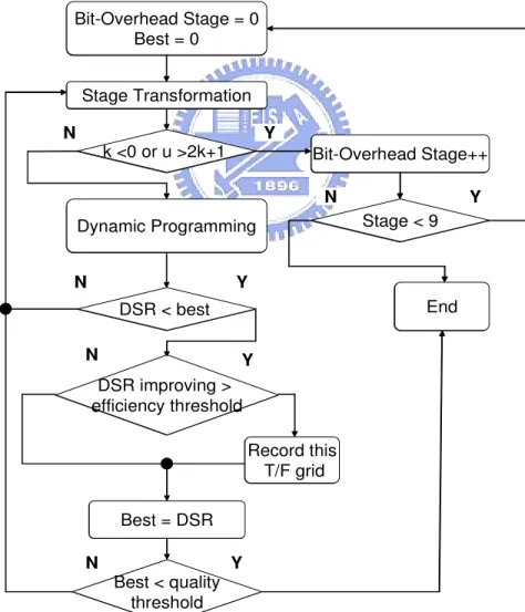
Through the above algorithm, the derived T/F grid presents that the error for this grid format is acceptable. However, the situation that no any T/F grid meets the quality constraint may happen. In such case, the highest resolution T/F grid may not the best solution. Therefore, another threshold is needed. This constraint is referred to as “efficiency threshold” because it restricts efficiency of consumed bits. The new form of T/F grid is adapted only when it improves some percentage over the best one. The efficiency constraint ensures that each additional time border and high resolution envelop is worth. The modified flow chart with efficiency threshold is illustrated in Figure 23. The proposed T/F grid decision take account of quality, bit overhead, and encoding bit rates at the same. The experiments in Chapter 6 will show the efficiency compared to other codecs.

Bit-Overhead Stage = 0 Best = 0 Stage Transformation Dynamic Programming k <0 or u >2k+1 N Y Bit-Overhead Stage++ Stage < 9 DSR < best Y N End Y N Record this T/F grid DSR improving > efficiency threshold Best = DSR Y N Best < quality threshold Y N Bit-Overhead Stage = 0 Best = 0 Stage Transformation Dynamic Programming k <0 or u >2k+1 N Y Bit-Overhead Stage++ Stage < 9 DSR < best Y N End Y N Record this T/F grid DSR improving > efficiency threshold Best = DSR Y N Best < quality threshold Y N

(42)

5.4 Frame Class Decision

Four frame classes are used in SBR codec. Each frame class has different flexibility to describe the distribution of time borders. According to the position of time borders, leading frame border and trailing frame border, frame class of each frame can be determined. In addition to record the format of time borders, the objective of frame class for variable frame border is to spare bits for time borders. If both frame borders are fixed, it means that there are two “time borders” wasted. In Figure 24(a), there are two consecutive frames and respective time borders. If the frame borders are always constant, the latter frame needs an extra time border. Comparing to Figure 24(b), due to the variable trailing frame border of the first frame, the first time border of the second frame can be removed.

T F 0 16 32 ( timeslots ) 32 0 18 FIX VAR (a) (b) T F 0 16 32 ( timeslots ) 32 0 18 FIX VAR (a) (b)

Figure 24: An example for variable frame border.

Consequently, in order to determine the position of the trailing frame border of each frame, the information for time borders of the next frame is necessary. According to looking ahead of the next frame and the distribution of time borders in this frame, the most suitable frame class can be determined.

(43)

Chapter 6 Artifacts in SBR

6.1 Tone Trembling

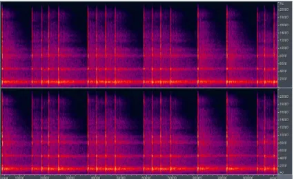
The patching which determines the corresponding relation between replicated low frequency bands and original high frequency bands is different depending on different master frequency band tables, SBR start and stop boundaries. If one of these three factors changes, then patching changes, i.e. assume that the 8th subband is replicated for someone high frequency subband this frame, and the next frame, the replicated low frequency subband change into 10th subband. This phenomenon may cause the spectrum discontinued in time domain. In noise-like signal, the discontinuous spectrum is hard to be discovered in both perceptual hearing and spectral envelope. However, in tone-rich signal, this phenomenon is much more serious. Comparing Figure 25(a) to Figure 25(b), and it is easy to see the discontinuity of spectrum. The major discontinued envelope locates on tones. In perceptual hearing, this artifact causes the signal sounds like trembling, or sparkling. Therefore, this phenomenon is referred to tone trembling artifact.

(a) (b)

(44)

6.2 Tone Shift

In tone-rich signal, the tone components usually distribute regularly. Figure 26 shows this phenomenon. In this kind of signal, using inverse filter and adding additional tone components is ineffective and bit-consuming. Furthermore, sinusoids in the frequency transform to signals with constant magnitude in the time domain. Therefore, the non-clipping method should be better than the clipping method either in time or frequency domain, i.e. no any time borders or additional components are needed. However, it will cause tone shift artifact in the reconstructed signal. This artifact is referred to “tone shift” because of its spectrum shape. In Figure 27, it shows this phenomenon. The blue line represents the spectrum of original signal, and the red one is reconstructed by HE-AAC. It is clear to see that, in SBR range, the tone components have offsets comparing to original ones, but they still keep regular. However, in the perceptual hearing, this artifact is almost hard to be discovered.

Figure 26: An example for characteristics of tone-rich signals

HE-AAC編碼器上之有效率的Time/Frequency Grid 設計

Efficient Design of Time/Frequency Grid in HE-AAC Encoder

Student Shou-Hung Tang

Advisor Chi-Min Liu

Wen-Chieh Lee

Efficient Design of Time/Frequency Grid in HE-AAC

Encoder

Contents

Figure List

Table List

Chapter 1

Introduction

Chapter 2

Backgrounds

2.1 SBR Decoder Overview

2.2 HF Generator

2.3 Envelope Adjuster

( )

(

)

( )

( )

(

)

( )

(

)

(

)

( )

( )

( )

(

) (

)

( )

(

)

( )

(

)

( )

( )

( )

( )

( )

( )

( )

( ) ( )

( )

( )

( ) ( )

( )

( )

( )

( )

(

( )

)

( )

( )

( )

( )

( )

( )

( )

( )

( )

( )

(

)

( )

(

)

[

]

( )

(

( )

( )

_{( )}

_{( )}

_{( )}