H.264/MPEG-4 AVC可調式視訊編碼之高資料效率預測演算法研究

國 立 交 通 大 學

電子工程學系 電子研究所碩士班

碩 士 論 文

H.264/MPEG-4 AVC 可調式視訊編碼之高資料效率預測演

算法研究

On the Data Efficient Prediction Algorithm for

H.264/MPEG-4 AVC Scalable Extension

研 究 生: 黃筱珊

指導教授: 張添烜

H.264/MPEG-4 AVC 可調式視訊編碼之高資料效率預測演

算法研究

On the Data Efficient Prediction Algorithm for

H.264/MPEG-4 AVC Scalable Extension

研 究 生: 黃筱珊 Student: Hsiao-Shan Huang 指導教授: 張添烜 博士 Advisor: Tian-Sheuan Chang

國 立 交 通 大 學 電子工程學系 電子研究所碩士班

碩 士 論 文

A Thesis

Submitted to Department of Electronics Engineering & Institute of Electronics College of Electrical and Computer Engineering

National Chiao Tung University in Partial Fulfillment of the Requirements

for the Degree of Master In

Electronics Engineering January 2010

Hsinchu, Taiwan, Republic of China

v

H.264/MPEG-4 AVC 可調式視訊編碼之高資料效率預測演算法研究

研究生: 黃筱珊 指導教授: 張添烜 博士 國立交通大學電子工程學系 電子研究所碩士班 摘 要 在設計可調式視訊編碼硬體的過程中，資料存取需求變成越來越困難，因 為採用了需要密集作資料存取的層間(inter-layer)預測模式。為了解決可調式視 訊編碼高資料存取量的問題進而達到編碼效能的提升。在這篇論文中，我們提出 三個適用在層間預測模式上的高資料效率的演算法。首先，我們提出一個把畫面 間(inter)預測和層間殘值(inter-layer residual)預測合併成一個預測程序的方法， 並且重複使用資料來減少資料存取需求。其次，我們提出一個高資料效率的層間 移動向量預測(inter-layer motion)演算法，藉由利用畫面間預測的參考資料來減 少層間移動向量預測的大量的參考資料需求，還有提供一個適用在層間基底 (inter-BL)預測的移動向量偵測機制，經由偵測層間基底的移動向量來決定參考 資料是否可以被重複使用。此外，在移動估測議題方面，我們也提出一個根據畫 面大小來適當調整的移動估計切換方法，藉由畫面的解析度大小適當地決定使用 平行化之解析度移動估測設計加上層間高資料效率預測演算法或是畫面間及層 間級別 C(level C)的資料重複使用演算法。模擬結果顯示在影像大小為 CIF 時， 傳輸資料率(bit-rate)僅有 0.16%的增加，而影像品質(PSNR)只有 0.002dB 的下 降; 在影像大小為 480p 時，傳輸資料率(bit-rate)則是 0.91%的增加，而影像品 質(PSNR)有 0.09dB 的下降。而以分析的結果來看，我們提出的方法可以在 CIF 以及 480p 的畫面大小下節省 67.3%和 80.9%的資料存取量。此資料存取節省 量，不只可提高系統編碼效能，更可以達到記憶體存取功率消耗的減少。

vii

On the Data Efficient Prediction Algorithm for H.264/MPEG-4

AVC Scalable Extension

Student: Hsiao-Shan Huang Advisor: Tian-Sheuan Chang

Department of Electronics Engineering & Institute of Electronics National Chiao Tung University

Abstract

Data access requirement becomes more and more critical in designing video coding hardware system especially for scalable video coding due to the adoption of inter-layer prediction with intensive data access requirement. In this thesis, we propose three data efficient prediction algorithms for inter-layer prediction to reduce the data access bandwidth. First, we introduce a method that combines inter and inter-layer residual predictions into one prediction process and reuse its data for lowering data access requirement. Second, a data efficient inter-layer motion prediction is presented by utilizing the reference data of inter prediction to further reduce the considerable reference data access. And a motion detection mechanism is proposed in inter-BL mode through perceiving the motion vector of inter-BL to decide that the reference data can be reused. Furthermore, for motion estimation issue, a frame size adaptive motion estimation switching method is also proposed in this thesis to adaptively determine the usage of the parallel multi-resolution motion

viii

estimation with data efficient inter-layer prediction algorithm or the level C data reuse scheme for both inter and inter-layer prediction algorithm by taking the frame resolution into consideration. Simulation results demonstrate that the average bit-rate increment is 0.16% and the PSNR degradation is 0.002dB in CIF sequences. For 480p sequences, the bit-rate increment is 0.91% and 0.09dB of PSNR degradation in average. However, analysis results show that the proposed method can save 67.3% and 80.9% data access requirement for CIF and 480p frame size, respectively. These data access saving not only can increase the coding speed of encoder but can save power consumptions brought by extreme data accesses for prediction.

ix

誌 謝

在交大碩士的生涯裡，感謝我的指導教授—張添烜博士，在研究所的生涯給 我的支持和鼓勵，教導我正確的研究態度，並學會解決問題。在研究上更讓我學 會許多研究的技巧，並在我遇到瓶頸時給予建議與協助。感謝老師提供豐富的實 驗室資源，讓我有個舒適的環境來充分利用各種軟硬體設備進行研究工作。老師 不僅是研究上的良師，也是生活上的益友。 感謝我的口試委員們，安霸股份有限公司蔣迪豪副總經理與交通大學電子工 程系李鎮宜教授。感謝你們百忙之中抽空前來指導，因為教授們的寶貴意見，讓 我的論文更加的充實而完備。 感謝 VSP 實驗室的好伙伴們，特別謝謝帶我入門的李國龍學長，從入門以來 到畢業前，都很細心的叮嚀我做研究的每一個步驟，包括作投影片的要點以及做 研究的態度，在我研究上提供極大的幫助。謝謝林佑昆(YK)學長和張彥中(Nelson) 學長，你們認真面對研究的態度，是我學習的好榜樣。謝謝曾宇晟(曾博)學長， 從修課到研究，總會時不時的叮嚀我該注意的小細節。感謝蔡宗憲(butz)學長、 詹景竹(bamboo)學長、戴瑋呈(小戴)學長與張瑋城(大瑋)學長，你們的負責任， 與研究上的無所不知，是我想學習的對象。感謝我的戰友們，陳之悠(大哥)、許 博淵(ado)、沈孟維(雄哥)、蔡政君(A 君)，除了在修課及研究上一起打拼之外， 一起出遊以及平時聊天、解悶、搞笑的記憶是讓人永遠不會忘記的。謝謝王國振 學長，以及廖元歆、陳宥辰、許博雄、陳奕均、洪瑩蓉、溫孟勳、曹克嘉、邱亮 齊、吳英佑等學弟妹，有你們的陪伴，讓我的研究生涯更豐富。感謝實驗室的所 有成員們，讓我的交大碩士生涯充滿寶貴的回憶。 感謝我的家人，我的爸爸、媽媽、姊姊在我研究生涯中，一直給我打氣加油， 在我做研究最低潮的時候，給我最大的支持與鼓勵，不論是電話還是 MSN 的關心 你們的支持是讓我完成學業的最大動力。

x

感謝仕捷，在我碩士生涯中，陪我度過困難，當我的垃圾桶，分享我的喜怒 哀樂。感謝薛涵方、黃佳堯、林仕涵，在我心情不好的時候，安慰我陪我談天說 地，度過低潮。

xi Contents

Chapter 1. Introduction ... 1

1.1. Motivation ... 1

1.2. Thesis Organization ... 2

Chapter 2. Overview of SVC Standard ... 3

2.1. Components of SVC Encoder ... 3

2.1.1. Intra-layer Prediction ... 4

2.1.2. Inter-layer Prediction ... 5

2.1.3. The Matching Criteria ... 7

2.2. Data Efficient Motion Estimation Algorithm ... 8

2.2.1. Level C Data Reuse Scheme for Full Search Motion Estimation [5] ... 8

2.2.2. Parallel Multi-Resolution Motion Estimation (PMRME) [6] ... 9

Chapter 3. Proposed Data Efficient Algorithm for INTER and ILR Prediction ... 13

3.1. Motivation: Efficient ILR Prediction Method ... 14

3.2. Proposed Data Reuse Prediction Method ... 14

3.2.1. Proposed Data Reuse Method for INTER and ILR Prediction ... 15

3.2.2. Adaptation of Fast ME Algorithm for Reducing Data Access Requirement ... 17

3.3. Simulation Results ... 20

xii

Chapter 4. Proposed Data Efficient Inter-layer Prediction Algorithms . 27

4.1. Data Efficient Inter-layer Motion Prediction Algorithm ... 27

4.1.1. Motivation: Analysis for Inter-layer Motion Prediction Algorithm ... 29

4.1.2. Proposed Data Reuse Inter-layer Motion Prediction Algorithm ... 35

4.2. Data Efficient Inter-BL Prediction Algorithm ... 37

4.2.1. Relationship Analysis for Inter-BL and Motion Vector Predictor ... 38

4.2.2. Proposed Data Reuse Inter-BL Prediction Algorithm ... 40

4.2.3. Combination of Data Reuse Inter-layer Residual Prediction Algorithm ... 41

4.3. Combined Data Efficient INTER and IL Prediction Algorithm ... 42

4.4. Simulation Results ... 49

4.5. Summary ... 55

Chapter 5. Conclusion and Future Work ... 57

5.1. Conclusion ... 57

5.2. Future work ... 58

xiii

List of Figures

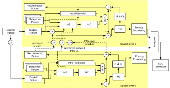
Fig. 2.1. Structure of SVC encoder ... 3

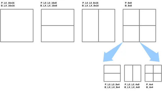
Fig. 2.2. Block partition of INTER prediction ... 5

Fig. 2.3. Prediction modes in SVC ... 5

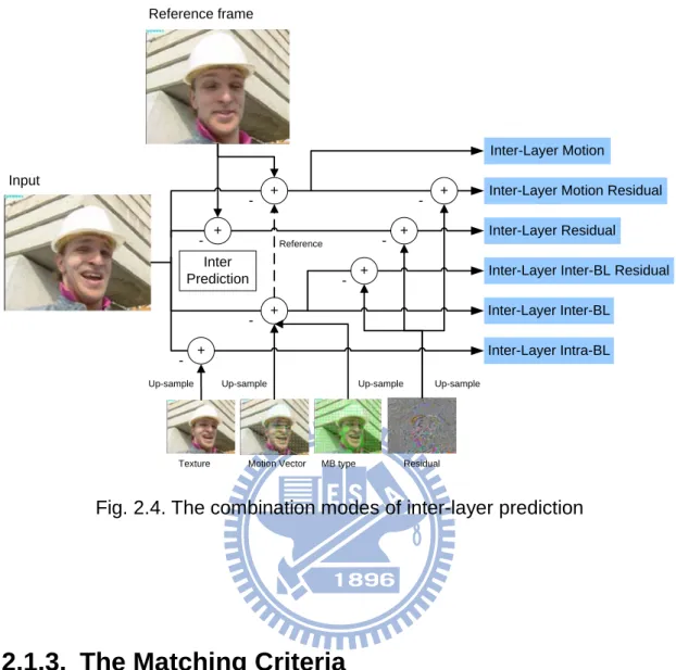
Fig. 2.4. The combination modes of inter-layer prediction ... 7

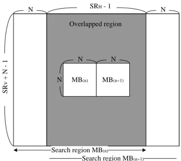
Fig. 2.5. The concept of Level C data reuse scheme ... 9

Fig. 2.6. Illustration of parallel multi-resolution motion estimation ... 10

Fig. 3.1. (a) INTER prediction process, (b) ILR process in JSVM reference software ... 13

Fig. 3.2. Proposed data reuse method which combines INTER and ILR prediction. ... 16

Fig. 3.3. Example of small-cross search algorithm ... 17

Fig. 3.4. Phenomenon of data overlapping of small-cross pattern ... 18

Fig. 3.5. The steps probability of SCS method ... 20

Fig. 3.6. Rate-Distortion curve of Football (a) QCIF (b) CIF ... 22

Fig. 3.7. Rate-Distortion curve of Silent (a) QCIF (b) CIF ... 23

Fig. 4.1. The reference data overlapped area of motion vector for INTER and inter-layer motion prediction ... 28

Fig. 4.2. The probability of MVP integer pixel difference between INTER and ILM predictions (a) vertical and (b) horizontal ... 30

Fig. 4.3. The probability of integer pixel difference between MVP of INTER prediction and MV of ILM prediction (a) vertical and (b) horizontal . 33 Fig. 4.4. Proposed inter-layer motion prediction algorithm. ... 37 Fig. 4.5. The probability of integer pixel difference between MVPINTER and

xiv

MVInterBL (a) vertical and (b) horizontal direction ... 39

Fig. 4.6. The flowchart of proposed data efficient inter-BL prediction algorithm ... 41 Fig. 4.7.The data access requirement in different frame resolutions ... 44 Fig. 4.8.The percentage of data access requirement in different frame

resolutions ... 44 Fig. 4.9.The flowchart of combined data efficient IL algorithms and dynamic

ME switching method... 45 Fig. 4.10.The flowchart of frame size adaptive ME switching method ... 46 Fig. 4.11.The flowchart of combined data efficient ILM algorithm and adaptive ME switching algorithm ... 47 Fig. 4.12.The flowchart of combining proposed data reuse Inter-BL algorithm

and adaptive ME switching algorithm ... 49 Fig. 4.13.The RD-curve of Level C + IL and PMRME + IL data reuse for CIF

sequences (a) Coastguard (b) Foreman ... 51 Fig. 4.14.The RD-curve of Level C + IL and PMRME + IL data reuse for 480p sequences (a) pedestrian_area (b) tractor ... 53

xv

List of Tables

Table 3.1. Simulation conditions ... 21 Table 3.2. PSNR degradation and bit-rate increase comparisons. ... 24 Table 4.1. The analysis results obtained by equation (4.2) ... 32 Table 4.2. The simulation results of two cases for 480p sequences (Blue_sky, Tractor, Station2, Pedestrain_area, Rush_hour, Riverbed) ... 35 Table 4.3. Data access requirement in different frame resolutions (Kbyte/frame) ... 43 Table 4.4. Simulation conditions ... 50 Table 4.5.The RD performance comparison of proposed data efficient IL

prediction algorithms with different ME approach for CIF sequences. ... 52 Table 4.6.The RD performance comparison of proposed data efficient IL

prediction algorithms with different ME approach for 480p sequences. ... 54

1

Chapter 1. Introduction

1.1. Motivation

Recently, video coding has been developed rapidly to satisfy diverse applications range from mobile device display to high-definition TV. Traditional video coding standards optimize the video quality at a given bit-rate without considering the variety of transmission environment. An extension of H.264/AVC called scalable video coding (SVC) [1] addresses this heterogeneous environment problem.

SVC is a newest video coding standard which standardized by Joint Video Team (JVT). In SVC, it supports three scalabilities, including temporal, spatial and quality scalability. Temporal scalability supports video coding in different frame rate by using hierarchical B structure. Quality scalability is achieved by Fine-Grain Scalability (FGS), Coarse-Grain Scalability (CGS) or Medium-Grain Scalability (MGS). Spatial scalability is provided by varying frame resolutions.

Due to similarities between spatial layers, inter-layer (IL) prediction is adopted in SVC for reducing the redundancy existed between spatial layers. However, the inclusion of IL prediction will additionally increase the memory bandwidth and computational requirements. Previous researches [2]-[4] have been proposed to reduce the computational complexity of SVC. However, they do not take the memory requirement issue into consideration. Since the memory access speed is far behind the data processing speed in modern video encoder design, the performance of designed video coding system is

2

totally dominated by memory access. As a result, lowering the memory bandwidth requirements not only improves coding performance of video coding system but reduces the power consumption brought by memory read/write access. Therefore, a prediction method of low data access requirement is proposed which combines inter prediction (INTER) (The term of “INTER” will be used as intra-layer inter prediction in the following contents.) and inter-layer residual (ILR) predictions into a single prediction module to deal with this problem. Furthermore, the data efficient inter-layer motion (ILM) and Inter-BL modes are also proposed to reduce the data access overhead by reusing the reference data of INTER prediction.

1.2. Thesis Organization

This thesis is organized with five Chapters. Chapter 1 introduces the motivation of this work. In Chapter 2, we briefly review the SVC prediction modes and motion estimation (ME) algorithms. Chapter 3 presents the proposed low data access method on INTER and ILR predictions. Chapter 4 describes the data efficient ILM and Inter-BL prediction algorithms combining with frame size adaptive ME switching method, and numerous simulation results are shown to demonstrate the efficiency of our proposed algorithms. Finally, the conclusion will be given in Chapter 5.

3

Chapter 2. Overview of SVC Standard

2.1. Components of SVC Encoder

Fig. 2.1 shows the basic structure of SVC encoder with two spatial layers. The base layer (BL) process the typical H.264/AVC encoder by using the intra-layer prediction mode. In the enhancement layer (EL), the intra-layer prediction is also adopted. However, for the high correlation between BL and EL, the IL prediction is supported by reusing the coding information from BL.

In the first step of encode process, the original input sequence is down-sampled N times to the demand size as the input sequence of BL as illustrated in Fig. 2.1. Then the BL sequence is encoded by typical H.264/AVC. Afterward, the EL is encoded by adopting inter-layer prediction which uses BL information as prediction reference. The BL information is up-sampled N times as EL prediction reference samples. In the following section, the intra-layer and inter-layer prediction modes are described in detail.

Original Picture Current Picture Reference Picture ME Intra Prediction + IT & IQ Entropy Encodering TQ Multiplex + Reconstructed Picture + -+ Current Picture Reference Picture + IT & IQ Entropy Encodering TQ + Reconstructed Picture -+ ↑N ↑N ↑N _{Spatial layer 1} Spatial layer 0 ↓N SVC bitstream Inter-layer residual Inter-layer motion &

Inter-BL Inter-layer texture MUX MC Intra Prediction ME MC MUX + + + +

4

2.1.1. Intra-layer Prediction

Intra-layer prediction includes intra prediction and INTER prediction mode. Intra prediction contains three different prediction modes for luminance block, including I_4x4, I_8x8, and I_16x16. I_4x4 and I_8x8 support 9 optional modes by copying the data of neighboring samples, and I_16x16 support 4 optional modes in the same way. For chrominance block, 4 optional modes are applied to intra prediction mode.

For INTER prediction mode, it can be future divided into uni-directional and bi-directional prediction by considering the List of the reference picture. The List refers to the previous coded picture before and after the current frame in display order. For example, uni-directional prediction adopts only list0 frame data, whereas bi-directional prediction adopts both list0 and list1 frame data as reference samples. Considering the ME, H.264/AVC defines the variable block size motion estimation (VBSME). In the uni-directional prediction, VBSME contains partition size ranging from 16x16 to 8x8, given the label of P_L0_16x16, P_L0_L0_16x8, P_L0_L0_8x16, P_L0_L0_8x8, respectively; In the bi-directional prediction, VBSME also contains partition size from 16x16 to 8x8, given the label of B_LX_16x16, B_LX_LX_16x8, B_LX_LX_8x16, B_LX_LX_8x8. The label “LX” refers to the index of list including L0, L1 and Bi. The 8x8 partition is future divided into 8x4, 4x8 and 4x4 modes as illustrated in Fig. 2.2.

5 P_L0_16x16 B_LX_16x16 P_L0_L0_16x8 B_LX_LX_16x8 P_L0_L0_8x16 B_LX_LX_8x16 P_8x8 B_8x8 P_L0_L0_8x4 B_LX_LX_8x4 P_L0_L0_4x8 B_LX_LX_4x8 P_4x4 B_4x4

Fig. 2.2. Block partition of INTER prediction

2.1.2. Inter-layer Prediction

Except inherent coding modes in the H.264, the SVC additionally supports IL prediction mode which uses reference layer information as the predictor to further reduce the redundancies existed between spatial layers.

Intra-layer prediction

Inter prediction Intra prediction

Inter-layer Residual prediction Inter-layer Motion prediction Base layer prediction Inter-layer prediction Intra-layer prediction Intra-layer prediction

Select the best prediction

Fig. 2.3. Prediction modes in SVC

6

modes, the intra and INTER predictions are the same as the prediction modes used in the H.264. For IL prediction, three type of prediction modes are defined, including ILR, ILM and base layer mode prediction. The base layer mode can be further classified to IL intra (Intra-BL) and Inter-BL prediction according to BL prediction modes. The Intra-BL reuses the up-sampled texture from base layer (BL) as reference samples for predicting the macroblock of enhancement layer (EL) when corresponding macroblock in BL is intra mode. For ILR prediction, the up-sampled BL residuals are subtracted from current data before performing motion estimation search. ILM prediction adopts the up-sampled motion of BL as motion vector predictor. Inter-BL is similar to inter-layer motion which uses the motion vector as well as partition mode of BL for prediction in enhancement layer. These inter-layer prediction modes can be combined with each other to efficiently utilize the BL information. The combination modes of IL prediction are shown in Fig. 2.4.

7

Input

Inter-Layer Motion

Inter-Layer Motion Residual Inter-Layer Residual Inter-Layer Inter-BL Residual Inter-Layer Inter-BL

Inter-Layer Intra-BL +

Up-sample

Texture Motion Vector MB type Residual +

+ +

+

Up-sample Up-sample Up-sample

+ + Reference -Reference frame Inter Prediction

Fig. 2.4. The combination modes of inter-layer prediction

2.1.3. The Matching Criteria

For selecting best mode, the final prediction mode is decided by RD_Cost. The function of RD_Cost is listed as follows:

,

R D

J = +λ• (2.1) where J represents RD_Cost, λ denotes Lagrangian parameter, D is distortion between current and reference data, and R refers to rate which is derived by computing the difference between selected motion vector (MV) and motion vector predictor (MVP).

8

2.2. Data Efficient Motion Estimation Algorithm

The ME becomes a major bottleneck when the search range is large which results in the massive data access. Therefore, a lot of data efficient ME algorithms have been proposed to solve this problem. In the following section, two ME algorithms are introduced which related to our proposed algorithm.

2.2.1. Level C Data Reuse Scheme for Full Search

Motion Estimation [5]

It is well-know that full search algorithm is the best ME method since it exhaustively searches all candidates within the search range. However, the large search range results in bandwidth bottleneck because of the massive data access. In order to solve this problem, Level C data reuse scheme was introduced while performing full search ME. Fig. 2.5 shows the concept of Level C data reuse scheme. When the search range is [-H, +H) in horizontal direction and [-V, +V) in vertical direction, the search range size is (SRH + N -

1)*(SRV + N - 1) where SRH = 2H, SRV = 2V, and N denotes the MB width and

height. The search range between neighboring macroblocks (MB) has lots of overlapped region. Hence, when the ME of MBn+1 is performed, the overlapped

region (SRV + N - 1)*(SRv + N - 1) of search range between MBn and MBn+1 is

reused and only N*(SRv + N - 1) additional data need to be loaded from external memory.

9 MB(n) MB(n+1) N N N N SRH - 1 N SR V + N - 1 Search region MB(n) Search region MB(n+1) Overlapped region

Fig. 2.5. The concept of Level C data reuse scheme

2.2.2. Parallel Multi-Resolution Motion Estimation

(PMRME) [6]

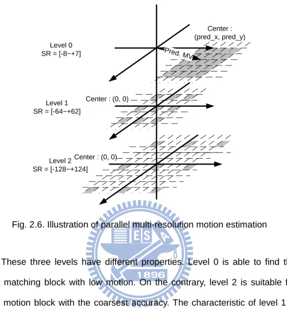
PMRME includes three levels. Level 0 is the same as full search algorithm which chooses the predictive motion vector as search center and exhaustively search the best result within search range [-8, +7]. Level 1 and level 2 are different from level 0 in which the search center are both located at (0, 0). Level 1 uses the 4:1 sampling and the search range is expanded to [-32, 30]. Level 2 uses the 16:1 sampling and the search range is [-128, 124]. The PMRME algorithm is shown in Fig. 2.6.

10 Pred. MV Level 0 SR = [-8~+7] Level 1 SR = [-64~+62] Level 2 SR = [-128~+124] Center : (0, 0) Center : (0, 0) Center : (pred_x, pred_y)

Fig. 2.6. Illustration of parallel multi-resolution motion estimation

These three levels have different properties. Level 0 is able to find the best matching block with low motion. On the contrary, level 2 is suitable for high motion block with the coarsest accuracy. The characteristic of level 1 is among the two levels mentioned above. Level 1 has smaller search range but finer accuracy compared with level 2.

The advantage of PMRME is that level 1 and level 2 are able to meet the data reuse scheme by restricting the search center at (0, 0). Furthermore, these two levels can improve the drawback of level 0 whose search range is too small to obtain the best matching result with high motion block.

Considering the data access requirement of Level C data reuse scheme, it produces considerable data access overhead when the search range is large although the data reuse scheme is applied. However, PMRME performs better

11

then Level C data reuse scheme when considering the data access issue due to the 4:1 and 16:1 sub-sampling with data reuse method. However, the penalty of PMRME is that the sub-sampling approach arises the degradation on the RD performance. The detailed comparisons of Level C and PMRME on data access issue and RD performance will be discussed in Chapter 4.

13

Chapter 3. Proposed Data Efficient

Algorithm for INTER and ILR Prediction

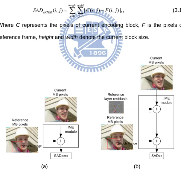
From previous overview, the final prediction mode is decided by RD_Cost, when computing the RD_Cost for INTER prediction mode, the D term in equation (2.1) is derived by calculating the sum of absolute difference of each block (DINTER), and it can be expressed as follows

,| ) , ( ) , ( | ) , ( 0 0

∑ ∑

= = − =height i width j INTER i j C i j F i j SAD , (3.1)

Where C represents the pixels of current encoding block, F is the pixels of reference frame, height and width denote the current block size.

Current MB pixels + Reference MB pixels SADINTER Search Range -IME module Current MB pixels + Reference MB pixels Search Range -Reference layer residuals SADILR + -IME module (a) (b)

Fig. 3.1. (a) INTER prediction process, (b) ILR process in JSVM reference software

14

In contrast to INTER prediction shown in Fig. 3.1(a), we can observe that the ILR prediction additionally substrates the up-sampled residual from current coding pixels before performing motion estimation search. Consequently, the

D term in equation (2.1) can be calculated as follows

∑ ∑

= = − − =height i width j ILR i j C i j B i j F i j SAD 0 0 |, ) , ( ) , ( ) , ( | ) , ( , (3.2)

When testing inter-layer residual prediction. B represents the base layer up-sampled residuals.

3.1. Motivation: Efficient ILR Prediction Method

From equations (3.1)-(3.2), it can be found that the main difference for calculating the D terms between INTER and IL prediction is that the IL prediction additionally substrates the up-sampled residual from current coding pixels. Based on this observation, it is possible to reuse the current and reference data when testing both INTER and IL prediction modes.

3.2. Proposed Data Reuse Prediction Method

In this chapter, our proposed data reuse method for INTER and ILR prediction is described in detail. Besides, a fast ME algorithm is also adopted to further reduce data access requirement in ME.

15

3.2.1. Proposed Data Reuse Method for INTER and ILR

Prediction

From chapter 3.1, we observed some identical processes existed between INTER and ILR prediction. Since the current MB data and the reference MB data of ILR prediction is the same as INTER prediction, the difference between these two prediction modes is that ILR mode needs one more process which subtracts up-sampled base layer residual from current coding pixels before performing integer motion estimation (IME). Motivated by this observation, we can combine these two prediction modes into one ME process and receive two prediction results at the same time. In other words, by changing the order of subtraction for DILR calculation, the equation (3.2) can be rewritten as follows.

∑ ∑

= = − − =height i width j ILR i j C i j F i j B i j SAD 0 0 | ) , ( ) , ( ) , ( | ) , ( , (3.3)

Through the equation (3.3), the DINTER can be derived by just extraction

the results of C-F during the computation of equation (3.3). Finally, both the results of DINTER and DILR can be obtained concurrently. The combined method

is shown in Fig. 3.2. When calculating the RD_Cost for the INTER prediction in IME module, we can perform ILR prediction at the same time by subtracting base layer residual. The advantage of our proposed method is that, in normal prediction process in the SVC, the current and reference pixels should be loaded twice for both INTER and ILR prediction. However, after the adoption of our proposal, the current and reference pixels only need to be loaded once for both prediction modes.

16 Current MB pixels + Reference MB pixels Search Range -Reference layer residuals SADILR + -IME module SADINTER

Fig. 3.2. Proposed data reuse method which combines INTER and ILR prediction.

To demonstrate the efficiency of our proposed method, we show some numerical comparisons of bandwidth saving for our proposal and full search motion estimation with level C data reuse scheme [5]. The data access requirements of full search ME for loading reference data in EL per frame can be calculated as follows ] 16 ) 15 2 [( ] ) 15 2 [(SR 2 MBl SR MBr DS_LevelC = × + × + × + × × , (3.4)

Where the MBl is the number of macro-blocks located at left most columns in a frame, the MBr is the number of macro-blocks per frame except the MBl, and

SR refers to the search range. For an example, the data access requirement of

full search ME algorithm with level C data reuse scheme in encoding CIF image (search range is equal to 16) can be calculated as follows.

Frame Kbypte DS_LevelC / 4 . 316 ] 378 16 ) 15 2 16 [( ] 18 ) 15 2 16 [( 2 = × × + × + × + × = , (3.5)

17

3.2.2. Adaptation of Fast ME Algorithm for Reducing

Data Access Requirement

For reducing computational complexity of ME, many fast motion estimation algorithms have been proposed to decrease the ME complexity such as three step search (3SS) [7] , four step search (4SS) [8] and diamond search (DS) [9]. But they are impractical to be realized by hardware, since data reuse is not effective and data access has no regular form. In this chapter, a fast motion algorithm technique called small-cross search (SCS) motion estimation [10] is selected for our proposed data efficient ME method due to its regular memory access, data reuse and simplicity properties for hardware realization.

Fig. 3.3. Example of small-cross search algorithm

Fig. 3.3 shows the concept of small-cross ME algorithm. The operation of this algorithm is described as follows. First, the SADs of five positions labeled by 1 are calculated. If the minimum SAD is located at center position, the search operation is finished and the coordinate of center position is set as

18

motion vector of current coding macro-block. Otherwise, the position with minimum SAD is set as the search center and another three additional positions labeled by 2 are checked. This operation is repeated until the position with minimum SAD is located at center or the search boundary is reached.

As described above that the small-cross search pattern can significantly reduce the computational complexity of ME. However, this search pattern not only can achieve computational complexity saving, but it can gain the benefit of data reuse from the perspective of hardware realization.

Fig. 3.4 shows the phenomenon of data overlapping of SCS pattern. In this figure, the light circles indicate the overlapped area and the dark circles of top row, bottom row, left column, and right column are referred to the additional required pixels for SAD calculation in case of the position with minimum SAD is located at position 1, 2, 4, and 5, respectively. From this figure, we can notice that there is large part of data overlapping between any two adjacent search positions. E D A B C 18 pixels 18 pixels

Fig. 3.4. Phenomenon of data overlapping of small-cross pattern

19

analyzed as follows. In the first step, there are five positions with 18x18 pixels should be downloaded from external memory for evaluation the SADs. If the minimum SAD located at center position, there is no more pixels should be downloaded from external memory. Otherwise, if the position with minimum

SAD located at any one of four corner positions, 18 addition pixels need to be

downloaded from external memory for evaluation. From the above analysis, we can observe that the data access requirements of small-cross pattern are proportional to the search steps. Therefore, the data access requirements per frame of small-cross search pattern can be calculated as follows

, )] 18 ( ) 18 18 [( N MBs DS_SCS = × + × × , (3.6) Where 18x18 indicates the required pixels for computing the SADs for first five positions, MBs denotes the number of macro-blocks in a frame and the N is the repeated steps for searching the best result.

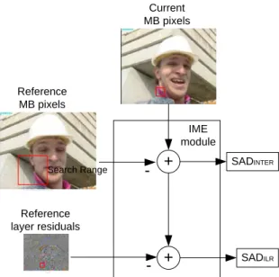
However, the steps in SCS are not fixed since it depends on sequence content. This property results in the difficulty for hardware implementation. From the memory requirement analysis mentioned above, we observed that the SCS might results in higher memory requirements than level C data reuse scheme when the search steps reach a certain number. In order to find out the average steps of SCS, some simulations are preformed. Fig. 3.5 shows the simulation results of SCS method.

20

Fig. 3.5. The steps probability of SCS method

The vertical and horizontal axes are the accumulated probability and search steps in SCS, respectively. Simulation shows that SCS method can find the best matching within 10 steps. Hence, we restricted SCS method to search 10 steps when realizing the SCS motion estimation algorithm. From equation (3.6), the data access requirement can be fixed to,

Frame Kbyte

DS_SCS =[(18×18)+(18×10)]×396=194.9 / , (3.7) in CIF size. There fore, 38.4% data access requirement can be reduced by

SCS method when compared to level C data reuse method if the ±16 search

range is adopted.

3.3. Simulation Results

The proposed algorithm is implemented on a JSVM8.9 [11]. The test condition is shown in Table 3.1.

21

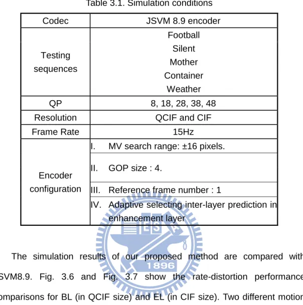
Table 3.1. Simulation conditions

Codec JSVM 8.9 encoder Testing sequences Football Silent Mother Container Weather QP 8, 18, 28, 38, 48

Resolution QCIF and CIF

Frame Rate 15Hz

Encoder configuration

I. MV search range: ±16 pixels. II. GOP size : 4.

III. Reference frame number : 1

IV. Adaptive selecting inter-layer prediction in enhancement layer

The simulation results of our proposed method are compared with JSVM8.9. Fig. 3.6 and Fig. 3.7 show the rate-distortion performance comparisons for BL (in QCIF size) and EL (in CIF size). Two different motion behavior sequences, Silent and Football are shown in figures. From these figures, we can observe that the proposed method can achieve near the same rate-distortion performance when compared to JSVM8.9. The detail comparisons for PSNR degradation and bit-rate increase are shown in Table 3.2. From this table, we observed that only 1.18% and 0.01 dB bit-rate increase and PSNR degradation in average for our proposed method, respectively. Furthermore, the memory bandwidth requirements can be saved up to 38.4% for all sequences in average.

22 Football(QCIF) 20 30 40 50 60 0 500 1000 1500 2000 Bit Rates(kbits/s) PS N R( dB ) JSVM Proposed (a) Football(CIF) 20 30 40 50 60 0 2000 4000 6000 8000 10000 Bit Rates(kbits/s) PS N R( dB ) JSVM Proposed (b)

23 Silent(QCIF) 20 30 40 50 60 0 100 200 300 400 500 600 Bit Rates(kbits/s) PS N R( dB ) JSVM Proposed (a) Silent(CIF) 20 30 40 50 60 0 500 1000 1500 2000 2500 3000 3500 Bit Rates(kbits/s) PS N R( dB ) JSVM Proposed (b)

24

Table 3.2. PSNR degradation and bit-rate increase comparisons.

Sequence Resolution QP 8 18 28 38 48 F oot ba ll QCIF △PSNR 0.033 0.022 -0.001 0.009 -0.123 △Bitrate(%) 0.485 1.118 2.208 3.880 5.364 CIF △PSNR 0.032 0.027 0.015 -0.003 -0.119 △Bitrate(%) 0.372 0.868 1.691 2.616 3.108 S ilent QCIF △PSNR 0.003 -0.002 -0.018 -0.008 -0.084 △Bitrate(%) 0.240 1.052 1.735 1.878 0.476 CIF △PSNR -0.001 -0.001 -0.004 -0.010 -0.069 △Bitrate(%) 0.205 0.753 1.168 1.377 -0.113 Mot h er QCIF △PSNR -0.030 -0.010 -0.014 -0.048 -0.064 △Bitrate(%) 0.351 0.749 2.013 3.944 1.313 CIF △PSNR 0.003 -0.018 -0.005 -0.039 -0.142 △Bitrate(%) 0.105 0.293 0.914 2.837 -0.549 C ont a in er QCIF △PSNR -0.007 -0.016 -0.034 -0.064 -0.128 △Bitrate(%) 0.061 -0.122 0.791 0.276 4.477 CIF △PSNR -0.002 -0.006 -0.019 -0.034 -0.076 △Bitrate(%) 0.042 -0.096 0.575 0.735 0.276 W ea ther QCIF △PSNR -0.011 -0.004 0.002 0.011 -0.015 △Bitrate(%) 0.221 0.624 1.857 3.654 4.187 CIF △PSNR 0.002 -0.002 -0.024 -0.014 -0.022 △Bitrate(%) 0.271 0.665 1.638 3.149 1.940 A v er age QCIF △PSNR 0.002 -0.002 -0.001 -0.015 -0.066 △Bitrate(%) 0.155 0.481 1.439 2.312 1.833 CIF △PSNR 0.005 0.000 -0.004 -0.022 -0.069 △Bitrate(%) 0.135 0.362 0.947 1.792 0.569

25

3.4. Summary

In this chapter, a data efficient prediction method is proposed to solve the problem of extreme data access demands brought by IL prediction of SVC. By combining both INTER and ILR prediction, the reference data for prediction can be reused efficiently. Simulation results show that the proposed method can save 38.4% data access requirement with slight rate-distortion performance degradation when compared to JSVM8.9.

27

Chapter 4. Proposed Data Efficient

Inter-layer Prediction Algorithms

In the following sections, the relation of MVs between INTER and IL predictions is performed. By the analysis, we discuss the dependency on MVs of these prediction modes. Thus, we propose several data reuse schemes used in IL by using the property of high correlation between INTER and IL prediction modes. With these methods, we can efficiently decrease the data access requirement in EL, and only increase the bit-rate within 0.16% and 0.002dB PSNR degradation in CIF sequences, and increases the bit-rate within 0.91% and 0.09dB PSNR degradation for 480p sequences in average when compared to JSVM 9.14.

4.1. Data Efficient Inter-layer Motion Prediction

Algorithm

From the spatial scalability perspective, we observed that the main difference between two successive spatial layers is only the sampling rate variation in spatial contents. In other words, the image contents of any continuous spatial layers may exist strong similarities between them and this property motivates us to find out the possibility whether the image data of

28

either layer can be reused by another layer or not. For example, if we can find out the situation that two prediction modes have highly correlated in its prediction references, we can reuse these prediction references and consequently reduce the data access overhead caused by different prediction modes. More concretely, Fig. 4.1 shows the concept of INTER and ILM prediction modes in EL. The dotted line refers to the search area of INTER prediction. The straight line represents the search area of ILM prediction. If the motion vector predictors of INTER (MVPINTER) and inter-layer motion (MVPILM)

are highly related, there will be significant portion of overlapped area covered by two search areas, as shown in Fig. 4.1 gray area, can be found out and these overlapped data can be shared by two prediction modes. Therefore, we have analyzed the relationship of MVPINTER and MVPILM since we suspect that

the MVPs between these two modes are quite close.

Enhancement layer Reference frame Inter-layer motion MVP INTER prediction MVP Overlapping area Search range of inter-layer

motion prediction

Search range of INTER prediction

Fig. 4.1. The reference data overlapped area of motion vector for INTER and inter-layer motion prediction

29

4.1.1. Motivation: Analysis for Inter-layer Motion

Prediction Algorithm

In this section, we analyze the relationship between MVPs of INTER and ILM predictions. Simulation result is shown in Fig. 4.2. In this figure, the horizontal axis denotes the MVP difference (mvp_diff) in integer pixel accuracy between INTER and ILM predictions and it can be calculated by the following equation.

mvp_diff = (MVPILM – MVPINTER) >>2, (4.1)

where the >>2 scales the motion vector accuracy from quarter pixel to integer pixel precision. The vertical axis stands for the accumulated probability. From this figure, we can observe that the accumulated probability can be reached up to 90% for all sequences both in vertical (Fig. 4.2 (a)) and horizontal (Fig. 4.2 (b)) directions if the MVP difference between INTER and ILM predictions is less than 8 pixels. Therefore, this simulation results tell us that it is highly possible to find out the best search result for either prediction mode from the reference data of another prediction mode due to the MVPs’ differences between two prediction modes are very small. Consequently, the search data of INTER and ILM can be shared for the prediction usage.

30 0.00% 10.00% 20.00% 30.00% 40.00% 50.00% 60.00% 70.00% 80.00% 90.00% 100.00% 0 4 8 12 16 20 24 28 32 Integer_pixel_difference(ver) Ac cum ul at ed pr oba bi lit y blue_sky sunflower station2 pedestrian_area rush_hour tractor riverbed average (a) 0.00% 10.00% 20.00% 30.00% 40.00% 50.00% 60.00% 70.00% 80.00% 90.00% 100.00% 0 4 8 12 16 20 24 28 32 Integer_pixel_difference(hor) Ac cum ul at ed pr oba bi lit y blue_sky sunflower station2 pedestrian_area rush_hour tractor riverbed average (b)

Fig. 4.2. The probability of MVP integer pixel difference between INTER and ILM predictions (a) vertical and (b) horizontal

31

From the analysis mentioned before, the MVP of INTER and ILM prediction modes is quite similar. Base on the reason that the INTER is adopted both in H.264 and SVC but the ILM prediction can be adaptively adopted in SVC, we can apply the same search area which uses INTER MVP as search center to both INTER and ILM prediction modes.

However, another question now is how to set the suitable search range that can achieve best data reuse rate for ILM prediction. In the following, we will discuss the relationship between MVP differences and best MV of inter-layer motion prediction (MVILM) to look for the suitable search range size

which can aim at optimal tradeoff between bandwidth reduction and rate distortion performance. To do so, we apply the conditional probability to analysis the relationship between MVP differences and MVILM by following

equation:

p(SR|s) = p(mvp_diff < SR | mvp_diff = s), (4.2)

where SR (1, 4, 8, 12, 16), s = [1~20]. ∈

In equation (4.2), mvp_diff is the MVP differences between INTER and ILM modes, and (MVILM – MVPINTER) < SR stands for whether the MVILM is located

within the search range, SR.

The analysis results obtained by the equation (4.2) is shown in

Table 4.1, and the graphical representation in vertical and horizontal directions are exhibited in Fig. 4.3(a) and Fig. 4.3(b), respectively. The horizontal axis is the integer pixel difference between MVPILM and MVPINTER; the vertical axis is

the probability of the integer pixel differences between MVILM and the MVPINTER

32

Table 4.1. The analysis results obtained by equation (4.2)

p(SR|s) in vertical direction p(SR|s) in horizontal direction

SR SR s 1 4 8 12 16 1 4 8 12 16 1 0.889 0.955 0.972 0.979 0.985 0.875 0.954 0.981 0.988 0.993 2 0.413 0.910 0.950 0.964 0.974 0.418 0.919 0.962 0.975 0.984 3 0.326 0.832 0.906 0.932 0.949 0.332 0.877 0.947 0.966 0.976 4 0.298 0.795 0.903 0.932 0.946 0.344 0.813 0.938 0.963 0.975 5 0.323 0.556 0.884 0.916 0.936 0.311 0.510 0.924 0.955 0.970 6 0.324 0.490 0.852 0.904 0.931 0.396 0.541 0.921 0.953 0.972 7 0.282 0.415 0.783 0.851 0.895 0.376 0.495 0.900 0.946 0.963 8 0.372 0.506 0.812 0.897 0.926 0.354 0.463 0.845 0.929 0.957 9 0.315 0.471 0.627 0.869 0.905 0.297 0.408 0.567 0.898 0.940 10 0.250 0.390 0.493 0.786 0.858 0.317 0.455 0.541 0.902 0.941 11 0.305 0.429 0.527 0.794 0.886 0.295 0.414 0.499 0.856 0.933 12 0.261 0.362 0.471 0.747 0.836 0.272 0.386 0.451 0.816 0.926 13 0.276 0.391 0.484 0.575 0.858 0.347 0.443 0.522 0.657 0.923 14 0.248 0.354 0.448 0.551 0.826 0.330 0.426 0.494 0.575 0.896 15 0.290 0.433 0.517 0.582 0.845 0.354 0.448 0.496 0.552 0.921 16 0.313 0.420 0.509 0.590 0.818 0.357 0.466 0.545 0.598 0.840 17 0.255 0.372 0.448 0.536 0.669 0.293 0.381 0.466 0.518 0.652 18 0.296 0.389 0.458 0.517 0.591 0.378 0.486 0.531 0.596 0.665 19 0.287 0.412 0.481 0.551 0.617 0.293 0.403 0.451 0.517 0.584 20 0.236 0.329 0.401 0.487 0.545 0.307 0.411 0.463 0.564 0.636

33 SR=8, 8 0.00% 10.00% 20.00% 30.00% 40.00% 50.00% 60.00% 70.00% 80.00% 90.00% 100.00% 1 2 3 4 5 6 7 8 9 10 11 12 13 14 15 16 17 18 19 20

integer_pixel_difference between MVPs (vertical)

p ro b a b il it y SR=1 SR=4 SR=8 SR=12 SR=16 (a) SR=8, 8 0.00% 10.00% 20.00% 30.00% 40.00% 50.00% 60.00% 70.00% 80.00% 90.00% 100.00% 1 2 3 4 5 6 7 8 9 10 11 12 13 14 15 16 17 18 19 20

integer_pixel_difference between MVPs (horizontal)

p ro b a b il it y SR=1 SR=4 SR=8 SR=12 SR=16 (b)

Fig. 4.3. The probability of integer pixel difference between MVP of INTER prediction and MV of ILM prediction (a) vertical and (b) horizontal

34

From this figure, we observed that when the search range is large, it is more probable that the best matching MVILM is inside the search range. For

example, when the search range is fixed to 16, the probability can reach 80% even the MVP difference is up to 16. However, for the case of search range fixed to 4, only the situation that the MVP difference less than 4 can reach 80%. Therefore, these simulation results demonstrate that the larger the search range size is, the more the final MVILM can be found within the same search

area of INTER prediction. Unfortunately, the larger search range size also implies the noticeable data access overhead. As a result, we choose a proper search range ±8 to achieve best tradeoff between lightening the bandwidth overhead and most coverage of best matching MVILM. Motivated by these

observations, a data efficient ILM prediction algorithm is developed by detecting the differences between MVPINTER and MVPILM.

From previous analysis, when the search range is fixed to ±8, the probability can reach 80% while the MVP difference is smaller than 8 pixels. Thus, we can set 8 as a threshold of MVP difference to develop our proposed algorithm. While the MVP difference is within the threshold, it can catch 80% probability without performance degradation due to the best MVILM can be

found within reused search area. However, the problem may exist when the MVP difference exceeds the threshold. There are two ways to solve this problem. First, the search mechanism for ILM is still performed with reused search area (case 1), the other way is to omit the search process for the ILM (case 2).

To evaluate the influence of above two situations, we performed some simulation to check the RD performance. The simulation result is shown in

35

Table 4.2.The QP is (28, 32), the frame size of BL and EL is CIF and 480p, respectively. From this table, the RD performance of these two conditions is almost the same. Therefore, through the simulation, we conclude that case 2 is better for the reason since it not only has ignorable RD performance degradation compared to case 1 but has less computation overhead.

Table 4.2. The simulation results of two cases for 480p sequences (Blue_sky, Tractor, Station2, Pedestrain_area, Rush_hour, Riverbed)

case 1 case 2

QP ΔPSNR Δ Bit-rate (%) ΔPSNR Δ Bit-rate (%) 28 -0.102 0.590 -0.103 0.575

32 -0.103 0.535 -0.103 0.540

4.1.2. Proposed

Data Reuse

Inter-layer Motion

Prediction Algorithm

As discussed above, when the MVP difference is smaller than threshold 8, significant amounts of ILM best matching MVILMs’ are located inside the ±8

search range. In addition, the simulation results show that the case 2 has only slight RD performance degradation and computational burden when compared to case 1. Therefore, an ILM data reuse algorithm is proposed by combining above two mentioned properties and its complete operating flow is described below.

36

As shown in Fig. 4.4, the IME starts finding the MVP of INTER and ILM prediction. After obtaining the MVPs, the MVP differences can be computed and compared to the threshold. The threshold is set to 8 in this thesis. If the MVP difference is smaller than the threshold, the [-8, +7] search range which centeredon MVPINTER is used for ILM prediction process as reference data to

find out the best prediction result. Otherwise, the ILM is skipped. The final step is to compare the RD_Costs between INTER and ILM modes and select the best mode which has minimum RD_Cost.

The proposed ILM algorithm described above has two contributions. The first is the efficient data reuse mechanism for the ILM prediction mode which can reduce the bandwidth overhead in coding the EL. The other profit is that the search range in ILM is only [-8, +7] which not only can save the computing time but can reduce power consumption during IL prediction.

37

Reuse reference data of INTER prediction for ILM

with SR [-8, +7]

Obtain the RD_Cost for ILM

Obtain the best mode Derive the

MVPINTER Derive the MVPILM

INTER prediction Y end N Load the reference data Skip ILM mode start mvp_diff < threshold Obtain the RD_Cost for INTER

Fig. 4.4. Proposed inter-layer motion prediction algorithm.

4.2. Data Efficient

Inter-BL

Prediction

Algorithm

In the previous section, we analyze the relation between MVs and MVP differences and propose a data reuse IL motion prediction algorithm. Since Inter-BL mode and ILM prediction mode have the same property that both of prediction modes using up-sampled MVs of BL for prediction, we further analyze the correlation between motion vectors of Inter-BL (MVInterBL) and

38

4.2.1. Relationship Analysis for Inter-BL and Motion

Vector Predictor

Fig. 4.5 shows the simulation results. In this figure, the horizontal axis denotes the difference (mv_diff) in integer pixel accuracy between MVPINTER

and MVInterBL and it can be calculated by the following equation.

mv_diff = Abs(MVInterBL – MVPINTER) >>2, (4.3)

where the >>2 scales the motion vector accuracy from quarter pixel to integer pixel precision. And the vertical axis stands for the accumulated probability. From this figure, we can observe that when the difference between MVPINTER and MVInterBL is smaller than 8 pixels, the probability can reach 90%

and 80% for vertical and horizontal direction in average, respectively. Since the Inter-BL mode has high probability to be selected as best mode in EL, to avoid great performance degradation, it is unreasonable to abandon this prediction mode as data efficient ILM prediction algorithm done in case of the reference data outside the search range. Therefore, based on such high correlation between MVPINTER and MVInterBL, we further propose an efficient Inter-BL

prediction algorithm by adding an additional checking mechanism which plays the role of determining whether the required reference data of Inter-BL prediction mode should be loaded from external memory or not.

39 0.00% 10.00% 20.00% 30.00% 40.00% 50.00% 60.00% 70.00% 80.00% 90.00% 100.00% 0 4 8 12 16 20 24 28 32 Integer_pixel_difference(ver) Ac cum ul at ed pr oba bi lit y blue_sky sunflower station2 pedestrian_area rush_hour tractor riverbed average (a) 0.00% 10.00% 20.00% 30.00% 40.00% 50.00% 60.00% 70.00% 80.00% 90.00% 100.00% 0 4 8 12 16 20 24 28 32 Integer_pixel_difference(hor) Ac cum ul at ed pr oba bi lit y blue_sky sunflower station2 pedestrian_area rush_hour tractor riverbed average (b)

Fig. 4.5. The probability of integer pixel difference between MVPINTER and

40

4.2.2. Proposed Data Reuse Inter-BL Prediction

Algorithm

Fig. 4.6 exhibits the flowchart of our proposed data efficient Inter-BL prediction algorithm. In the first step, the Inter-BL mode gets the number of partitions from the corresponding block in BL for current MB. Next, the MV of partition n (MVInterBL_n) is checked through the motion detection mechanism.

When the difference between MVPINTER and MVInterBL_n is less than or equal to

the threshold, the search data of INTER prediction mode are reused to derive the necessary data for Inter-BL prediction mode. Otherwise, when the MVInterBL_n exceeds the threshold, the additional required data are loaded from

external memory for Inter-BL prediction. The process is repeated until the MVInterBLs’ of all partitions are checked. The final step is to compare the

RD_Costs between INTER and Inter-BL modes and select the best mode

which has minimum RD_Cost.

The proposed data reuse Inter-BL algorithm described above has the contribution of reusing the reference data of INTER prediction since there is high probability that the required reference data of Inter-BL is inside the search window of INTER prediction. The only penalty is that the addition of a motion detection module.

41

Reuse reference data of INTER prediction

For Inter-BL

Obtain the RD_Cost for

partition n

Obtain the best mode

Obtain the RD_Cost for

INTER Derive the MVPINTER

INTER prediction Y end N Load the reference data Derive Mbpartition, n=0 Y Loaded reference data from external

memory

n = n+1 Accumulate the

RD_Cost

N

Derive MVInterBL for partition n; MVInterBL_n

start

n < MBpartition

mv_diff < threshold

Fig. 4.6. The flowchart of proposed data efficient inter-BL prediction algorithm

4.2.3. Combination of Data Reuse Inter-layer Residual

Prediction Algorithm

The data reuse of ILR prediction is mentioned in the previous chapter. In this section, we also combine the ILR prediction to achieve a complete data

42

efficient IL prediction.

As describe in Chapter 3, when calculating the RD_Cost for the INTER prediction in IME module, we can perform ILR prediction at the same time by subtracting base layer residuals. Similarly, when calculating the RD_Cost for the ILM and Inter-BL prediction, we can also perform ILR prediction at the same time.

4.3. Combined Data Efficient INTER and IL

Prediction Algorithm

From previous description, we proposed a data efficient ILM and an Inter-BL prediction algorithm to solve the problem of bandwidth overhead and computational complexity. However, the data access requirement of INTER prediction has also to be discussed in this thesis since all our proposed data efficient IL algorithms have reused the reference data of INTER prediction.For reducing the data access requirement, the level C data reuse scheme has been widely adopted in designing motion estimator. Nevertheless, the data access requirement of level C data reuse scheme becomes noticeable when search range larger than ±64 for SD/HD sequences. Therefore, the reference data subsample motion estimation algorithm called PMRME was proposed to solve the reference data access intensive problem. As a result, we analyze the data access requirement for these two methods (level C data reuse scheme and PMRME) and choose the best one which can achieve least data access requirement when combined with our proposed inter-layer prediction

43

algorithms. Table 4.3 shows the analysis results of data access requirements, and the statistic chart is shown in Fig. 4.7. The IL data reuse denotes the whether the reference data of INTER is reused in IL mode. The Level C data reuse scheme with IL data reuse denotes that the Level C data reuse scheme is applied for INTER mode to load reference data and IL prediction reuses INTER mode’s reference data. Otherwise, the reference data of IL centered at MVPILM is loaded from external memory without data reuse. When the PMRME

with IL data reuse is adopted, it represents the [-8, +7] reference data of INTER mode is reused. Otherwise, the reference data of all IL prediction modes are loaded from external memory without data reuse. To future compare the data access with different cases, the percentage of data access requirement is shown in Fig. 4.7. The result shows that when the resolution is smaller or equal to CIF size, level C data reuse scheme for both INTER and IL prediction is preferred. Otherwise, when the resolution is larger or equal to 480p size, the PMRME with IL data reuse algorithm is a better choice.

Table 4.3. Data access requirement in different frame resolutions (Kbyte/frame)

1

Compared to Method 1

IL data reuse QCIF CIF 480p 4CIF 720p 1080p

Level C N (Method 1) 173.77 1300.16 10626.66 12472.60 83592.05 636766.44 Y (Method 2) 78.63 425.39 2201.31 2586.85 9975.65 41894.34

PMRME N (Method 3) 215.62 1435.77 10525.77 12351.20 80243.69 617101.49 Y (Method 4) 115.67 541.74 2034.76 2388.41 6452.18 21835.40

1

44

Data access requirement

1 10 100 1000 10000 100000 1000000

QCIF CIF 480p 4CIF 720p 1080p Resolution Log s c al e ( K by te/ fr am e) Method 1 Method 2 Method 3 Method 4

Fig. 4.7.The data access requirement in different frame resolutions

Data access requirement

0% 20% 40% 60% 80% 100% 120% 140%

QCIF CIF 480p 4CIF 720p 1080p

Resolution P er c ent age Method 1 Method 2 Method 3 Method 4

Fig. 4.8.The percentage of data access requirement in different frame resolutions

45

Therefore, we choose Level C data reuse scheme for both INTER and proposed IL data reuse algorithms when the resolution is smaller than or equal to CIF size. Otherwise, the PMRME with proposed IL data reuse algorithms is selected as proposed algorithm.

The combination of proposed algorithm is shown in Fig. 4.9. In the first step, the INTER prediction process is executed and the reference data corresponding to different ME algorithm would be loaded into internal memory. Afterward, the reference data of INTER prediction can be reused during the ILM and Inter-BL process. Finally, the best mode is selected by comparing the

RD_Cost. The detailed flow charts of these three modules are described

below.

end start

Frame adaptive ME switching method for

INTER prediction

Obtain the

RD_Cost for INTER

Proposed data efficient ILM

algorithm

Obtain the

RD_Cost for ILM

Proposed data reuse Inter-BL algorithm

Obtain the

RD_Cost for

Inter-BL

Obtain the best mode

Fig. 4.9.The flowchart of combined data efficient IL algorithms and dynamic ME switching method

46

Fig. 4.10 is our proposed frame size adaptive ME switch algorithm. The ME algorithm is determined by the frame resolution. When the frame resolution is larger than or equal to 480p, we choose the PMRME algorithm for the reason that the data access requirement of PMRME is less than Level C scheme. Otherwise, the Level C scheme is selected in ME operation.

Obtain the

RD_Cost for

INTER mode

Derive the MVPINTER

INTER prediction

Load the reference data by

Level C scheme start

Derive the MVPINTER

Load the reference data for PMRME algorithm

end

Y N

Frame resolution >= 480p

Fig. 4.10.The flowchart of frame size adaptive ME switching method

As mentioned in the previous section, the ILM mode is able to reuse the reference data of INTER mode. Since the INTER prediction adopts frame size adaptive ME switching method, the reference data is distinct when choosing different ME algorithms. Therefore, the data efficient ILM algorithm is altered rely on the ME algorithm. Fig. 4.11 shows flowchart of the combined data efficient ILM algorithm and adaptive ME switching algorithm. When the frame

47

resolution is larger than or equal to 480p, the PMRME is used in INTER process. The difference between MVPILM and MVPINTER is checked to

determine whether reference data of INTER prediction with [-8, +7] search range size would be reused by ILM mode or not. When the Level C data reuse scheme is selected in INTER process, the entire reference data existed in internal memory can be efficiently used for ILM mode.

Reuse reference data of INTER prediction for ILM

with SR [-8, +7]

Obtain the

RD_Cost for ILM

Derive the MVPILM

start

Y N

Derive the MVPILM

Reuse reference data of INTER prediction for ILM

with Level C scheme

end Frame resolution >= 480p Y N Skip ILM mode mvp_diff < threshold

Fig. 4.11.The flowchart of combined data efficient ILM algorithm and adaptive ME switching algorithm

For Inter-BL mode, the data efficient algorithm is adopted with a motion detection mechanism. The detection is based on a threshold which related to the search range of reference data. The flowchart of combined data efficient Inter-BL algorithm and adaptive ME switching algorithm is shown in Fig. 4.12.

48

When PMRME is used, the threshold is set to 8 because the reference data is available within the search window of INTER prediction mode. Otherwise, the threshold is set to the search range size of Level C scheme due to the reference data is existed inside the search range. After setting the threshold, the motion detection mechanism is performed for each partition. When the partition n of MVInterBL_n is less than or equal to the threshold, it implies that the

reference data is already existed and can be reused. If the partition n of MVInterBL_n is over the threshold, it is necessary to load the reference data from

49

Reuse reference data of INTER prediction

For Inter-BL mode Obtain the RD_Cost for partition n Y end N Derive Mbpartition, n=0 Y

Loaded reference data from external memory

n = n+1

Accumulate the

RD_Cost

N

Derive MVInterBL for

partition n; MVInterBL_n n < MBpartition mv_diff < threshold start Y N Frame resolution >= 480p threshold = 8,Apply PMRME algorithm threshold = SR, Apply Level C ME algorithm

Fig. 4.12.The flowchart of combining proposed data reuse Inter-BL algorithm and adaptive ME switching algorithm

4.4. Simulation Results

The proposed algorithms are implemented on a JSVM9.14 [12], and the simulation conditions are shown in Table 4.4.

50

Table 4.4. Simulation conditions

Codec JSVM 9.14 encoder

Test sequences

Akiyo, Coastguard, Container, Foreman, Mobile, Silent, Blue_sky, Tractor, Station2,

Pedestrain_area, Rush_hour, Riverbed

QP 16, 20, 24, 28, 32

Resolution QCIF and CIF

CIF and 480p

Frame Rate 15Hz

Encoder configuration

I. MV search range: ±16, ±32pixels. II. GOP size : 8.

III. Reference frame number : 1

IV. INTER prediction search algorithm with Level C and PMRME

V. Proposed IL prediction algorithm in enhancement layer

Fig. 4.13 and Fig. 4.14 show the RD performance in CIF and 480p size sequences, respectively. Table 4.5 and Table 4.6 show the detailed RD performance comparison. The simulation results show that, when compared to JSVM 9.14, the RD performance is 0.16% in bit-rate increase and 0.002dB in PSNR degradation for CIF sequences when the search algorithm is full search with Level C data reuse scheme for INTER prediction and reference data reuse for IL prediction, and the RD performance is 0.91% in bit-rate increase and 0.09dB in PSNR degradation in 480p sequences if the PMRME search algorithm with data efficient IL prediction method is applied.

51 Coastguard_CIF 30.000 32.000 34.000 36.000 38.000 40.000 42.000 44.000 46.000 0 500 1000 1500 2000 2500 3000 3500 Bit-rate (Kbit/sec) PSN R JSVM9.14

LevelC + IL data reuse PMRME + IL data reuse

Foreman_CIF 30.000 32.000 34.000 36.000 38.000 40.000 42.000 44.000 46.000 48.000 0 200 400 600 800 1000 1200 1400 1600 1800 2000 Bit-rate (Kbit/sec) PSN R JSVM9.14

LevelC + IL data reuse PMRME + IL data reuse

Fig. 4.13.The RD-curve of Level C + IL and PMRME + IL data reuse for CIF sequences (a) Coastguard (b) Foreman

52

Table 4.5.The RD performance comparison of proposed data efficient IL prediction algorithms with different ME approach for CIF sequences.

CIF sequences@15Hz QP 16 20 24 28 32 Akiyo Level C ΔPSNR -0.003 -0.002 -0.003 -0.001 -0.001 ΔBitrate(%) -0.007 -0.029 -0.166 0.180 0.116 PMRME ΔPSNR -0.036 -0.052 -0.064 -0.063 -0.104 ΔBitrate (%) 0.660 0.816 1.157 1.706 1.547 Coastguard Level C ΔPSNR -0.001 -0.003 -0.004 -0.010 -0.015 ΔBitrate (%) 0.385 0.506 0.614 1.045 1.293 PMRME ΔPSNR -0.031 -0.037 -0.048 -0.054 -0.056 ΔBitrate (%) 0.376 0.445 0.493 0.580 0.781 Container Level C ΔPSNR 0.001 -0.003 0.000 -0.002 -0.008 ΔBitrate (%) -0.010 0.031 -0.041 -0.026 -0.128 PMRME ΔPSNR -0.027 -0.027 -0.039 -0.053 -0.049 ΔBitrate (%) 0.231 0.695 0.797 0.927 1.313 Foreman Level C ΔPSNR 0.000 -0.006 -0.002 -0.016 0.000 ΔBitrate (%) 0.112 0.175 0.259 0.158 0.335 PMRME ΔPSNR -0.105 -0.130 -0.155 -0.180 -0.180 ΔBitrate (%) 1.388 1.978 2.318 2.480 2.478 Mobile Level C ΔPSNR 0.001 0.002 -0.003 0.003 0.000 ΔBitrate (%) -0.001 0.014 -0.044 -0.026 -0.105 PMRME ΔPSNR -0.051 -0.053 -0.070 -0.079 -0.084 ΔBitrate (%) 0.547 0.667 0.852 1.197 1.553 Stefan Level C ΔPSNR 0.033 0.029 0.008 -0.028 -0.059 ΔBitrate (%) 2.787 3.977 5.090 5.928 6.811 PMRME ΔPSNR -0.053 -0.049 -0.058 -0.089 -0.108 ΔBitrate (%) 0.569 0.925 1.476 1.660 2.376 Average Level C ΔPSNR 0.000 -0.002 -0.002 -0.005 -0.004 ΔBitrate (%) 0.092 0.120 0.089 0.228 0.276 PMRME ΔPSNR -0.051 -0.061 -0.076 -0.085 -0.090 ΔBitrate (%) 0.719 0.978 1.149 1.355 1.415

Level C average : ΔBitrate = 0.161%, ΔPSNR = -0.002 dB PMRME average : ΔBitrate = 1.123%, ΔPSNR = -0.073 dB