多台攝影機監視系統下的物體追蹤與對應

國 立 交 通 大 學

電子工程學系 電子研究所碩士班

碩

士

論

文

多台攝影機監視系統下的物體追蹤與對應

Moving Objects Tracking and Correspondence over

Multi-Camera Surveillance System

研 究 生：王郁晴

指導教授：王聖智 博士

多台攝影機監視系統下的物體追蹤與對應

Moving Objects Tracking and Correspondence over

Multi-Camera Surveillance System

研 究 生：王郁晴 Student：Yu-Ching Wang

指導教授：王聖智博士 Advisor：Dr. Sheng-Jyh Wang

國 立 交 通 大 學

電子工程學系 電子研究所碩士班

碩 士 論 文

A Thesis

Submitted to Department of Electronics Engineering & Institute of Electronics College of Electrical and Computer Engineering

National Chiao Tung University in partial Fulfillment of the Requirements

for the Degree of Master in

Electronics Engineering June 2007

Hsinchu, Taiwan, Republic of China

多台攝影機監視系統下的物體追蹤與對應

研究生：王郁晴 指導教授：王聖智 博士

國立交通大學

電子工程學系 電子研究所碩士班

摘要

在本文中

，

我們提出了一個基於三維粒子濾波器的多物體追蹤及對應

技術，利用多個二維物體追蹤的結果，建立起物體在三維空間中的機率分

佈，並透過二維三維資訊的交換，更新及預測這個分佈的變化。同時，這

個三維的機率分佈，也可以幫助我們修正二維追蹤的結果，以及建立起各

視野間物體的對應關係，並且能夠自動的修正錯誤的對應關係。有了物體

的對應關係，就可以解決物體交錯所造成的追蹤錯誤，並且能夠更加正確

的估測三維物體的機率分佈，使多物體的追蹤和對應更加準確而可靠。

Moving Objects Tracking and Correspondence over

Multi-Camera Surveillance System

Student :Yu-Ching Wang Advisor : Dr. Sheng-Jyh Wang

Department of Electronics Engineering, Institute of Electronics

National Chiao Tung University

Abstract

In this thesis, we propose a 3-D particle filter based objects tracking and

correspondence system. Through the 2-D tracking results, we can predict and

update the probability distribution of moving objects in 3-D domain. With such

probability, we can not only refine the 2-D tracking results but also construct

the correspondence of objects in different camera views. In addition, our

system is able to correct the correspondence automatically based on some 2-D

and 3-D clues. With the object correspondence, the occlusion problem can be

solved easily and the 3-D probability distribution of moving objects can also

be estimated more precisely. These advantages make the results of objects

tracking and correspondence more robust and reliable.

誌謝

我很慶幸當初決定來交大念研究所，能和指導教授 王聖智老師以及實驗

室的成員們一起做研究。實驗室的氣氛融洽，每星期大家都會一起打球，

有問題也會互相幫助，就像是一個大家庭，使我能很快融入新的學習環

境。我很喜歡每星期的 group meeting，除了可以瞭解其他人的研究，一起

討論，更可以磨練自己的表達能力。在此特別感謝王聖智老師，他總是站

在學生的立場為我們著想，且對學生完全的信任。每每在研究遇到瓶頸的

時候，老師都能適時的給予很多新的想法以及方向，透過不斷的討論和驗

證，解決原本始終想不透的問題。讓我瞭解到要如何從無到有，解決一個

困難的問題。這兩年來的日子，除了培養了研究的能力，更使我變得有自

信且自動自發。

Contents

Chapter 1 Introduction ... 1 Chapter 2 Backgrounds ... 3 2.1 Motion Detection... 3 2.1.1 Background Subtraction... 3 2.1.2 Temporal Differencing ... 5 2.1.3 Optical Flow... 6 2.1.4 Learned Classifier ... 6 2.2 Motion Tracking... 8 2.2.1 Region-Based Tracking ... 8 2.2.2 Active-Contour-Based Tracking... 9 2.2.3 Model-Based Tracking ... 10 2.2.4 Feature-Based Tracking... 11 2.2.4.1 Mean-Shift... 12 2.2.4.2 Particle Filter ... 13 2.3 Multi-Camera Correspondence ... 14 2.3.1 Region-Based Methods ... 14 2.3.2 Point-Based Methods ... 14

Chapter 3 Proposed Method ... 20

3.1 2-D Objects Detection and Tracking ... 21

3.1.1 Background Subtraction Detection ... 21

3.1.2 Mapping Objects ... 23

3.2 Transformation Between 2-D and 3-D ... 25

3.3 3-D Particle Filter... 27

3.3.1 Particle Filter Algorithm... 27

3.3.2 Proposed 3-D Particle Filter... 31

3.3.2.1 First Generation of Particles... 31

3.3.2.2 Correction of Particles... 33

3.3.2.3 Shrink of Particles ... 35

3.3.2.4 Prediction of Particles ... 37

3.4 Information Exchange Between 2-D and 3-D... 40

3.4.1.1 First Construction of Correspondence... 40

3.4.1.2 Correspondence Update ... 43

3.4.2 Occlusion Handling... 45

3.5 Overall System Structure ... 47

Chapter 4 Experimental Results ... 48

Chapter 5 Conclusion ... 56

List of Tables

Table 3-1 algorithm of particle filter[28] ... 29

Table 3-2 algorithm of resampling [28] ... 30

List of Figures

Figure 1-1 Multi-camera surveillance system... 1

Figure 2-1 Horprasert T’s method [2] ... 4

Figure 2-2 The illustration of the results before and after Gabor Filters [5]... 5

Figure 2-3 The example of detection result by applying Gabor Filters [5]... 5

Figure 2-4 Training data[6] ... 6

Figure 2-5 A example of training features[6] ... 7

Figure 2-6The original image[8] ... 8

Figure 2-7 The example of Wren’s region-based tracking method ... 8

Figure 2-8 The example of McKenna’s region-based tracking algorithm [9]... 9

Figure 2-9 The example of Paragios’s active-contour-based algorithm[10] ... 9

Figure 2-10 3-D generic model[11]... 10

Figure 2-11 Different models of human body [12] ... 10

Figure 2-12 An example of color histogram [20]... 11

Figure 2-13 The illustration of the convergence of mean-shift... 12

Figure 2-14 the concept of particle filter... 13

Figure 2-15 The comparison of mean-shift and particle filter[20]... 13

Figure 2-16 An example of indoor surveillance system[23] ... 15

Figure 2-17 An example of Utsumi’s method [23] ... 15

Figure 2-18 The illustration of correspondence in 3-D domain by Utsumi’s method[23]... 16

Figure 2-19 The illustration of epipole constraint [24] ... 17

Figure 2-20 Black, Jamesa’s correspondence method based on the epipole constraint [24] .... 17

Figure 2-21 S. Khan’s correspondence in 2-D method [25] ... 18

Figure 2-22 An example of J. Black’s method [26] ... 19

Figure 3-1 a posterior process of background subtraction ... 21

Figure 3-2 The results before and after the morphological operations ... 22

Figure 3-3a illustration of objects detection applied in our system ... 22

Figure 3-4 the illustration of all kinds of tracking results ... 24

Figure 3-5 a illustration of camera setup[27] ... 25

Figure 3-6 a illustration of particle filter ... 27

Figure 3-7 a illustration of resampling ... 30

Figure 3-8 a illustration of tree... 31

Figure 3-10 3-D particles and the centers of gravity after shrink ... 36

Figure 3-11 2-D tracking results and the illustration of 3-D particles ... 38

Figure 3-12 Extra particles for new entering objects ... 39

Figure 3-13 extra particles for the objects still not establishing the correspondence relation. ... 39

Figure 3-14 a illustration of fuzzy adjustment ... 46

Figure 3-15 the flow chart of our system ... 47

Figure 4-1 the tracking and correspondence results in seq1 under occlusions ... 50

Figure 4-2 modification of size by a fuzzy adjustment (Seq1) ... 50

Figure 4-3 modification of size by a fuzzy adjustment (Seq2) ... 51

Figure 4-4 the demonstration of self-correction of our system ... 53

Figure 4-5 the establishment of the correspondence relation for detected new object ... 54

Chapter 1 Introduction

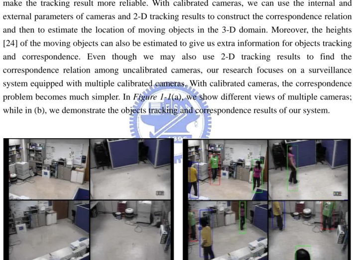
Surveillance systems have attracted more and more attention in recent years. With an intelligent surveillance system, we can automatically detect and track moving objects. Furthermore, we can recognize one person’s identity and decide the occurrence of an abnormal event. Based on the number of cameras, surveillance systems can be classified into single-camera surveillance systems and multi-camera surveillance systems. A single-camera surveillance system cannot handle the occlusion problem whereas a multi-camera surveillance system can integrate the information from several cameras to solve this occlusion problem and make the tracking result more reliable. With calibrated cameras, we can use the internal and external parameters of cameras and 2-D tracking results to construct the correspondence relation and then to estimate the location of moving objects in the 3-D domain. Moreover, the heights [24] of the moving objects can also be estimated to give us extra information for objects tracking and correspondence. Even though we may also use 2-D tracking results to find the correspondence relation among uncalibrated cameras, our research focuses on a surveillance system equipped with multiple calibrated cameras. With calibrated cameras, the correspondence problem becomes much simpler. In Figure 1-1(a), we show different views of multiple cameras; while in (b), we demonstrate the objects tracking and correspondence results of our system.

(a)The environment of our surveillance system (b)Objects tracking and correspondence of our surveillance system

In this thesis, we propose a 3-D particle filter based objects tracking and correspondence system. The main idea is that the motion detection problem can be described as a probability distribution problem. Here, we assign higher probability values at those 3D positions where some moving objects are likely to be present. Since the probability distribution of moving objects in the 3-D domain may not be Gaussian distribution, we use a group of particles to approximate this distribution. Moreover, since this distribution combines all the information from different camera views, it can refine the 2-D tracking results and construct the correspondence relation by back-projecting all 3-D particles onto 2-D image planes. When the correspondence has been constructed, the occlusion problem in 2-D image planes can be solved easily by fusing other camera views’ 2-D tracking results, which belong to the same 3-D moving object. In addition, we can classify all the 3-D particles into different moving objects in the 3-D domain. The major advantage is that we will neither just focus on the moving objects which have the most 3-D particles nor ignore the ones which have the fewest 3-D particles. By exchanging information between 2-D domain and 3-D domain, our system can automatically check if the correspondence relation is correct. The number of the 3-D particles varies dynamically according to the correspondence results. For example, if there is an object in a 2-D image plane which cannot build the correspondence with other camera’ views, we will give more particles along the path where this object may appear in the 3-D domain. Also, if some 2-D image planes detect new objects, we will use the same method to generate 3-D particles. By adjusting the number of 3-D particles adaptively, we can dynamically update the 3-D probability distribution of moving objects and make our system more flexible and robust.

Chapter 2 Backgrounds

In this chapter, we will introduce some existing methods for moving objects detection, tracking and correspondence. In 2.1 and 2.2, we will integrate and discuss some moving objects detection and tracking methods, which are popular in recent years. In 2.3, we will discuss some methods which focus on how to fuse the information from different view of cameras and how to establish the correspondence of moving objects in each camera view.

2.1 Motion Detection

In this section, some popular methods about how to detect moving objects in a complex background are to be discussed. The detection process is very important since better detection algorithms support better tracking and correspondence results. Since all of these methods have advantages and disadvantages, we usually choose a suitable algorithm according to the environment of the surveillance system.

2.1.1 Background Subtraction

Background subtraction is a method to detect moving regions in an image by taking the difference between the current image and the reference background in a pixel-by-pixel fashion. This technique is developed especially for surveillance systems with static cameras since the reference background model is needed. After subtraction, each pixel of residuals is then classified as foreground if its intensity is larger than a given threshold; otherwise the pixel is classified as background. Although this method is quite simple and costs low computation, it is very sensitive to the image noise and the variation of illumination. Stauffer [1] uses a set of Gaussian distributions to represent a pixel’s value. In other words, the intensity at each pixel in the reference background follows the distribution of a Gaussian mixture model (GMM). The difference between the current image and the reference background is obtained by measuring the distance of each point to its corresponded set of Gaussian distributions. Moreover, the parameters of Gaussian distributions will be adjusted as time goes on. As a result, the background model becomes more precisely and flexibly. However, the detection results are still degenerated by shadows and highlights. Horprasert T [2] utilizes the concept of color constancy of human eyes to separate the information of color and intensity. It can not only segment the moving regions in an image but also tell if some pixels of the moving regions belong to shadows or highlights. As

Figure 2-1 shows, the upper-left picture is the reference background and the upper-right picture

is the current image. In the lower-left figure, the blue region represents the detected moving object, and the red region indicates the shadows and highlights. The lower-right picture shows the final result of detection.

Figure 2-1 Horprasert’s method [2]

Upper-left is the reference background, upper-right is the current image. In the lower-left picture, the blue region is the detected moving object and red region is shadows and highlights. The lower-right picture is the final detection result.

Duque [3] takes the temporal differencing results into consideration. The detected moving regions obtained by both temporal differencing results and background subtraction results can reduce the influence of noise.

2.1.2 Temporal Differencing

Temporal differencing is a method to detect moving regions by taking the difference between successive images. We can use a given threshold to distinguish moving parts from static parts. Although this approach needs low computation and is not sensitive to the environment, it can only detect moving objects. That is, if an object stops to move, then it will be misclassified as a part of background. In addition, sometimes the detection results are not reliable because the detected regions are usually not complete and have many holes. Fu-Yuan Hu [4] does some morphological operations and GMM detection on the results of temporal differencing to eliminate these holes. S Dubuisson [5] uses a particular set of Gabor filters to filter the residuals. The contribution of such filters is to emphasize the moving regions. As Figure 2-2 shows, the left figure illustrates the original result, and the right figure shows the results after using Gaber filters. After the filtering, we put some particles randomly on the moving regions, with the number of particles being proportional to the magnitude of motion. As Figure 2-3 shows, in the left figure the white particles represent the locations with larger motion. By applying some classification methods, we can cluster the small residuals to accomplish the detection task.

Figure 2-2 The illustration of the results before and after Gabor Filters [5]

Left one is the original results of time differencing, and right one is the results after applying Gabor filters.

Figure 2-3 The example of detection result by applying Gabor Filters [5]

Left figure is the detection results after applying Gabor filters, white particles represent the points used to clustering, and the right figure shows the final detection results.

2.1.3 Optical Flow

Optical flow is a method to represent each pixel by a function of time and location. If along the time a moving point only changes its location while keeps its intensity values unchanged, then we can estimate its motion vector. The pro of this method is that we can extract moving objects from the background even over a dynamic camera system. In addition, by classifying the motion vectors of each pixel we can further segment and distinguish different moving objects. The con of this method is that it costs a lot of computation and is not suitable for real-time surveillance systems.

2.1.4 Learned Classifier

Learned Classifier method needs to know the objects which are going to detect. That means we need to train a set of classifiers at first based on the features of objects. Figure 2-4 illustrates some examples of training data for detection. However, there are lots of features that can be selected to train the classifiers and Figure 2-5 illustrates one of the selections. The pro is that if the amount of the training data is large enough then the performance of this method can be very good. In addition, the application of this method is not limited to static camera systems. The con is that this method can only detect specific kinds of objects and it needs a large amount of training data to “learn” these objects. V Nair [6] proposes a method which doesn’t require much training data at first. Instead, his system can learn the features of objects online by combining the motion information of the moving objects. Hence, his system can learn the objects’ features adaptively.

Figure 2-4 Training data[6]

The left figure shows some training examples of “people”. The right figure shows some training examples of “background”.

Figure 2-5 A example of training features[6]

Many detection methods contain more than one working principle. For example, Dongxiang Zhou [7] proposes a method which integrated all the aforementioned concepts. Since each method has its pros and cons, we may combine different methods to achieve better detection results.

2.2

Motion Tracking

In the previous section, we have introduced several detection methods. In this section, motion tracking methods are to be discussed. Motion tracking is to track moving objects from one frame to another in an image sequence and it is the key process of a surveillance system. Some major types of motion tracking techniques will be introduced in the following sections.

2.2.1 Region-Based Tracking

The basic component of a region-based tracking algorithm is a segmented region, called blob. The main idea is to track such a region in successive frames of an image sequence. Generally speaking, these kinds of tracking algorithms utilize the background subtraction to detect objects in the first place. Wren [8] describes the detected objects as small blobs. As Figure

2-7 shows, by comparing the value with the reference GMM background model, each pixel of

the foreground can be further classified into the corresponding blob. Then we can successfully track the object by tracking all of its small blobs.

Figure 2-6The original image[8] Figure 2-7 The example of Wren’s region-based tracking method.

The 2-D illustration of small blobs belongs to the same object [8]

McKenna [9] also uses the background subtraction technique to get the regions which possibly belong to the parts of moving objects and uses bounding boxes to select these regions. As shown in Figure 2-8, the left picture shows the original results of background subtraction, and the middle picture shows the results after classification. Each bounding box contains a part of moving object. The right picture illustrates the final results of McKenna’s algorithm. Based on the structures and color models of human bodies, we are able to classify the regions into different persons. Moreover, if the region involves only one person then it is denoted as “people”; otherwise, if it involves more than one human body, it will be denoted as “group”. The task of objects tracking can be accomplished by analyzing and tracking these regions. By comparing the color information with their color models, moving objects can be tracked successfully without

losing their identities even if these objects are partially occluded.

Figure 2-8 The example of McKenna’s region-based tracking algorithm [9]

The left figure is the result of background subtraction, and the middle figure shows the segmentation of residuals which are marked by rectangles. There are three regions and two of them belong to the same person. The right one is the final tracking result.

2.2.2Active-Contour-Based Tracking

Active-contour tracking method is to track objects by representing their outlines as bounding contours and updating these contours over time. Paragios [10] tracks the moving objects in an image using a geodesic active contour objective function and a level-set formulation scheme. In Figure 2-9, there is a convergent process of active-contour-based algorithm. Active-contour-based algorithms can represent the moving objects more precisely than region-based algorithms. However, this method requires perfect detection results and needs manual selection at first. Consequently, it is difficult to start this kind of systems automatically.

2.2.3 Model-Based Tracking

Model-based tracking algorithms need to build the prior structure models of the objects at first and then build the model for each candidate of target. Moving objects are tracked by matching the prior model with the model of the target candidates. The definition of rigid objects and non-rigid objects are quite different. Rigid objects such as cars can be tracked by comparing their 3D generic models with the reference models [11], as shown in Figure 2-10 . On the other hand, the models of non-rigid objects, such as human bodies, are more difficult to build due to the possible deformations. Some models of human body [12] are shown in Figure 2-11. Model-based tracking methods usually need to maintain a lot of parameters to build the models. Hence, it is difficult to implement these model-based tracking methods due to their heavy computational loads. However, if we use fewer parameters to build the models, then these models may not be able to describe the objects precisely.

Figure 2-10 3-D generic model[11]

The left figure shows some 3-D generic models of cars. The middle and the right figures show the models of the detected cars.

（a） （b） （c）

Figure 2-11 Different models of human body [12]

（a）stick-figure model of human body（Chen and Lee, 1995） （b）2-D contour model of human body（Leung and Yang, 1994）（c）volumetric model of human body（Hogg, 1994）

2.2.4 Feature-Based Tracking

The main idea of feature-based tracking algorithm is to extract the features of moving objects for tracking. By comparing the features in an image sequence, the task of tracking is successfully done. Based on different features, the algorithms can be further classified as global feature-based methods, such as center of gravity[13], color[14], area[15]; local feature-based methods, such as line[16], vertex[17]; and dependence-graph-based methods, such as the change of structures among features.

Nowadays many real-time surveillance systems adopt feature-based algorithms for objects tracking. Mean-shift method [19] and particle filter [21] are two popular algorithms. Generally speaking, color is the common feature for these two algorithms. The tracked objects are modeled in terms of their color histograms. Color histogram is to calculate the color distribution of a selected area. As shown in Figure 2-12, (a) is the color histogram of the target calculated from the region inside the green rectangle, while (b) is the color histogram of the candidate calculated from the region inside the red rectangle. By comparing the color histogram with the reference color model, moving objects can be tracked since the same objects should have similar color distributions. * q _{( )} k k q x （a） （b）

Figure 2-12 An example of color histogram [20]

（a）color histogram of the target（b）color histogram of the candidate

Bhattacharyya distance is a popular similarity measure of color histogram. The value of similarity measure is obtained by multiplying the color histograms of the reference model and the detected object in a point-by-point fashion and then summing up the products. The value of the similarity measure ranges from 0 to 1, with a larger value indicating a more similar matching. The advantage of color histogram is that it keeps the information of the target even if the target object is under expansion, shrink, rotation, or deformation. In addition, it requires low expense of computation. In the following section, we will introduce the mean-shift algorithm and particle filter, respectively.

2.2.4.1 Mean-Shift Algorithm

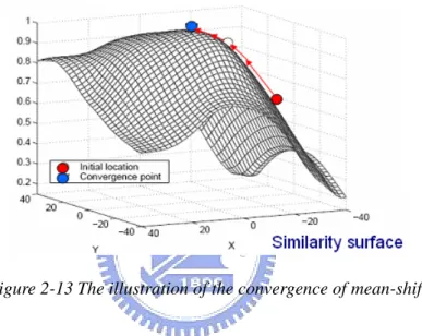
Mean-shift is a mathematic tool used to find the local maximum of any known or unknown distribution. As long as we have the well definition of object model such as color histogram and appropriate similarity measure such as Bhattacharyya coefficient, mean-shift can help us search for the top of the distribution to achieve the task of object tracking in an image sequence. In Figure 2-13, the surface is constructed by calculating the similarity between each point and its corresponding point in the reference model. The red point is the initial position and it will converge to the blue point which is the estimated position of moving object after applying mean-shift algorithm.

Figure 2-13 The illustration of the convergence of mean-shift

This method is appropriate to be applied to real-time surveillance system due to its low computation. However, since mean-shift algorithm can only find the local maximum, it must be careful to choose the initial position otherwise it will converge to the wrong position. So the system using mean-shift algorithm for objects tracking must have self-correction ability. That means it can detect and correct the wrong tracking result automatically to make the performance robust and reliable.

2.2.4.2 Particle Filter

If the moving objects in an image can be described as a probability distribution, then we can task the moving objects successfully by maintaining such a distribution precisely in an image sequence. Unfortunately, it is hard to estimate and update the distributions dynamically since these kinds of distributions usually do not belong to linear or Gaussian distributions. Particle filter algorithm provides a solution for such problem by using a group of particles to approximate the distribution. Through the prediction and update of each particle’s weight, the distribution of moving objects will be described correctly over time. As shown in Figure 2-14, the position of each black point which is so-called particle sampled form the objects’ distribution represents the possible position of the moving object. Each particle has different weight based on its similarity with the target model. The final position of moving object, the white point, is estimated by calculating the center of gravity of all these particles.

Figure 2-14 the concept of particle filter

The pro of particle filter algorithm is that the moving objects are described as a probability distribution approximated by lots of particles so the system has more chance to find the right positions of objects even under short-time occlusions. In Figure 2-15, top row shows the result of mean-shift algorithm while bottom row shows the result of particle filter and the red bounding box represents the final decision whereas yellow bounding box represents the decision of each particle with different weight. It is clear that the particle filter algorithm gives the better results than mean-shift algorithm.

Figure 2-15 The comparison of mean-shift and particle filter[20]

2.3

Multi-Camera Correspondence

In previous sections, we have introduced how to detect and track moving objects over single-camera surveillance system. In the following section, we are going to introduce how to track moving objects and construct the correspondence between multiple cameras. The system will have a broader view for objects tracking trough the cooperation of multiple cameras. In addition, when the correspondence relation has been established, the system will overcome some problems which are not able to be solved in single-camera surveillance system such as occlusions. Multi-camera correspondence can be roughly classified into region-based method and point-based method.

2.3.1 Region-Based Methods

Region-based methods usually represent the moving objects in an image as regions in one camera view and then compare the features of these regions with other regions in anther camera view to construct the correspondence relations. Color information is the popular feature used to establish the correspondence such as color histogram [21] or GMM color model [22]. Although this method is really simple, it is not reliable due to the variation of illumination. Also, the color information of objects in different camera views has an important impact on the correspondence result. For example, if two persons in different camera views dressed in the clothes with same color or two sides of clothes are different colors, it is easy to make mistakes in objects correspondence.

2.3.2 Point-Based Methods

Point-based methods construct the correspondence by comparing the features between different camera views based on some constraints of cameras. According to different geometric constraints, we can classify the methods into correspondence in 2-D domain and correspondence in 3-D domain.

The concept of correspondence in 3-D domain is shown in Figure 2-16. The left figure is an example of indoor surveillance system and the right figure shows the top view of this indoor environment where the cameras mounted on the ceilings in a circle. Each camera monitors one view and then transmits the 2-D information of that view to 3-D domain. By fusing all 2-D information coming from cameras of different views, we can roughly estimate the positions of objects in 3-D domain. The correspondence relations are able to be constructed by back-projecting the 3-D estimations into each 2-D image plane. However, this method needs the camera calibration before the system starts to work.

Figure 2-16 An example of indoor surveillance system[23]

Utsumi [23] finds the COG (center of gravity) of the detected objects in each 2-D image plane. The points inside a detected region are called COG if they have the longest distances to their closest boundaries As shown in Figure 2-17, the left is the original residual after detection and the right figure illustrates the distance map of the residual and the black points are so-called COG. How to find the correspondence relations by COGs? First of all, we project COGs from all camera views to 3-D domain and use the Gaussian distributions to estimate the positions of objects in 3-D domain. Through the back-projection of 3-D Gaussian distributions to all 2-D image planes, we can compare the detected COGs with the projected COGs in each camera view to find the possible correspondence relations.

Figure 2-17 An example of Utsumi’s method [23]

The left one is the original residual. And the right one is the distance map where the black points are so-called COG.

Figure 2-18 The illustration of correspondence in 3-D domain by Utsumi’s method[23] The objects are modeled as Gaussian distributions with N

(

Xh1,Sh1

)

in 3-D domain

where X_h1and S_h1 are mean and covariance of Gaussian distribution respectively. It is sill a Gaussian distribution after back-projection from 3-D to 2-D.

Black, Jamesa [24] uses the constraints of epipole plane to correspond objects in different camera views. As shown in Figure 2-19 it is an illustration of epipole plane where m1 and m2 are obtained by back-projecting the 3-D object located at M on image plane 1 and image plane 2 respectively. The back-projection lines, Mm1 and Mm2, will go through Es1 and Es2 which are camera focuses. The epipole plane constraint tells us that Es1, Es2 and M are in the same 2-D plane called epipole plane and m2 will lay on ep11 which is the intersection line of epipole plane and image plane 2.

Based on the epipole constraint, the center of each detected object in a 2-D image can project a line called epipole line on a 2-D image of another camera view and this epipole line will go through the center of the corresponding object belonging to the same 3-D object in that camera view. However, there may be some errors of 2-D tracking results. So the center of the corresponding object could not lay on the epipole line exactly. By combing this constraint and the 2-D tracking results, the task of multi-objects correspondence can be achieved.

Figure 2-19 The illustration of epipole constraint [24]

Es1,Es2 are focuses of camera1 and camera2, M is the position of object in 3-D domain ,m1,m2are the back-projection of M to image plane 1 and image plane 2 respectively, and ep11 is the intersection line of epipole plane and image plane 2.

Figure 2-20 Black, Jamesa’s correspondence method based on the epipole constraint [24] There are epipole lines with different colors in four images above. T he color of the epipole lines of detected object in image1 is red and green, blue, and yellow are the colors of the epipole lines of image2, image3,and image4 respectively. The green rectangles in image and image4 are ground plane regions, and the yellow rectangles in image2 and image3 are occlusion plane regions.

The correspondence method in 2-D domain doesn’t need the calibrated cameras. It only needs some clues of 2-D images in different camera views to find the correspondence relations. S. Khan [25] finds the overlap regions of current image and other images of different camera views. Only when the moving object appears in such overlap regions, it has the correspondence relation to the objects detected in other camera views. As shown in Figure 2-20, the range of each camera

view is shown in the left figure and the grey point represents the object. We can find that the object is visible in camera2’s view but invisible in camera3’s view. The right figure is camera1’s view and the region of other camera’s views projecting on it.

Figure 2-21 S. Khan’s correspondence in 2-D method [25]

The left figure illustrates the ranges of three camera views The right figures is the camera1’s view. There are some lines indicated the regions of the overlap views from other camera’s views. We can easily find that the black point in the bottom of object is visible in camera1’s view and camera2’s view but invisible in camera3’s view.

J. Black [26] is to find the homography matrix between two 2-D images of different camera views. With this matrix, we can transform any point of current camera view to the point of another camera view. This method is much easier than the method using the epipple constraint. As shown in Figure 2-22, the blue lines are epipole lines and red points are the correspondence points using homography matrix transformation.

Figure 2-22 An example of J. Black’s method [26]

Viewpoint correspondence using: epipole line analysis and homography alignment

The tasks of multi-objects correspondence in both 2-D domain and 3-D domain are hard due to that the results are easier degraded due to the influence of noise or the inaccuracy of 2-D tracking results.

Chapter 3

Proposed Method

In a multi-camera surveillance system, if we know the exact positions of moving objects in the 3-D domain, then the 2-D image planes are just the back-projection of the 3-D data onto different camera views. In other words, if we can track objects successfully in the 3-D domain, then the 2-D objects tracking problem is solved automatically. In practical situations, however, we only have 2-D images. Since the 2-D images have lost the depth information when projecting the 3-D objects onto 2-D images, it is difficult to deal with the occlusion problem when two or more objects are closer to one another. Hence, in our study, we try to find a method to combine the 2-D tracking results from different views of cameras and use the camera geometry constraints to estimate the 3-D positions of the moving objects.

In this thesis, we use a group of 3-D particles with different weights to describe the probability distribution of moving objects in the 3-D domain. This probability distribution can be constructed and updated by 2-D tracking results. In addition, this probability distribution can also help the refinement of the 2-D tracking results since it fuses the information coming from all camera views. The multi-objects correspondence can be established by some clues obtained by back-projecting all 3-D particles onto the 2-D image planes of different camera views. The correspondence relations will help us to solve the occlusion problem which is hard to be accomplished in single-camera surveillance systems. Besides, the establishment of correspondence is also an important clue for 3-D particles’ classification and then the probability distribution will be more accurate to describe the moving objects in 3-D domain. The advantage of classification for 3-D particles is that the distribution will not only focus on some specific objects having better tracking results in 2-D image planes. When new objects enter, the probability distribution should be updated as soon as possible. So we can put extra 3-D particles along the paths where the objects may appear in 3-D domain based on the clues coming from the current 2-D tracking results. In addition, if the objects in some 2-D image planes are still not able to establish the correspondence relations, we can use the same method mentioned above to update the probability distribution. Consequently, the number of 3-D particles is variable which depends on the current situation. Moreover, our system has the ability to correct the correspondence relations automatically to make performance more robust and reliable.

3.1 2-D Objects Detection and Tracking

In this section, we will discuss the method of 2-D objects tracking applied in our system. Each image of the sequence is applied background subtraction for objects detection. Then by comparing and connecting the detection results between successive images, the task of objects tracking is accomplished successfully.

3.1.1 Background Subtraction Detection

Since our system belongs to the static-camera surveillance system, we can build the reference background model for each camera view before starting the system. Then we can extract the foreground by taking the difference between current image and the reference background in a point-by-point fashion. However, the residuals are neither complete nor correct and need to do some posterior processing due to the influence of noise, variation of illuminations, and shadows. First of all, we use a given threshold of intensity to remove some noise and apply the method proposed in [3] to reduce the influence of illuminations and shadows. As shown in

Figure 3-1, (a) is the residuals after a given threshold, (b) indicates the illuminations and

shadows, and (c) is the final result obtained by eliminating noise, illuminations and shadows. It is clear that the influence of the shadows is reduced in this example.

(a) the residuals after a given threshold

(b) illuminations and shadows (c) final result Figure 3-1 a posterior process of background subtraction

Then we apply the morphological operations to fill the holes to make the residuals more complete. As shown in Figure 3-2, figure (a) and (b) are the results before and after the

(a) the results before the morphological operations

(b) the results after the morphological operations

Figure 3-2 The results before and after the morphological operations

Sometimes there is more than one object in an image. So we need to segment the objects from the residuals. First, we sum the residuals vertically to get the profile of moving objects in x-direction. The height of profile is proportion to the probability of moving objects appearance. So we can use a given threshold to eliminate some noise of the profile to segment the moving objects in x-direction, get the width of each moving object, and calculate the number of moving objects in that image. This process is shown in Figure 3-3 (a). Then we can sum the residuals in each segmented region horizontally to get the length of each moving object. Finally, each moving object in the image is marked as a bounding box as shown in Figure 3-3 (b). However,

when two or more objects in an image become too closer, they will be detected as one object since there is no extra information to separate them.

(a)an example of vertical summation of the residual.

(b)final result

3.1.2Mapping Objects

Through the method mentioned above, we can do objects detection for each image. In order to do objects tracking, the detection result of each image should be connected in time domain. Our objects tracking method is to compare the detection results between successive images to correspond the moving objects in time domain. The concept can be explained by Figure 3-4. Left column is the illustration of all possible tracking results between successive images and the red rectangle represents the detected object at time t-1 while blue rectangle represents the detected object at time t. We can establish the correspondence relations of moving objects in time domain by analyzing their overlap regions. Right column represents the correspondence tables of moving objects at time t-1 and time t. Figure (a) is the one to one case where the moving objects at time t-1 correspond to different objects at time t respectively, figure (b) is the mergence case where the moving objects become closer at time t-1 and then merge to the same object at time t, figure (c) is the split case where the moving object at time t-1 splits into two objects at time t, figure (d) is the new objects case where there are more moving objects at time t than time t-1, and figure (e) is the leave case where some of moving objects at time t-1 disappear at time t.

(a)one to one

(b)mergence

(d)new objects

(e) leave

Figure 3-4 the illustration of all kinds of tracking results

Through this way, we can track the moving objects in an image sequence and get the relations of these moving objects such as mergence, split, or new objects entering etc. It provides the useful information for multi-camera correspondence which will be discussed in the following sections. .

3.2Transformation Between 2-D and 3-D

Before using multiple cameras for objects tracking and correspondence, the geometric relations between cameras should be established at first. With such relations we can project the 2-D tracking results into 3-D domain and then fuse the information to achieve the cooperation of multiple cameras for objects tracking and correspondence. After camera calibration, we can get the intrinsic and extrinsic parameters of cameras which can be used for transforming the information between 2-D domain and 3-D domain. Figure 3-5(a) illustrates the world coordinate of PTZ camera. and are the rotation center and projection center of camera respectively,

is the new projection center after the camera tilts R

O O_C

'

O_C φ degree and r is rotation radius of

camera.

(a)model of camera setup (b)geometry of a horizontal plane with respect to a rectified camera and a tilted camera.

Figure 3-5 a illustration of camera setup[27]

Each camera has its own world coordinate and some intrinsic and extrinsic parameters obtained by camera calibration. With these parameters we can easily transform information between 2-D and 3-D domain. Also we can get the rotation matrix and translation vectors for transformation between different world coordinates. The formula of transformation from 3-D to 2-D is as follows, ⎥ ⎥ ⎥ ⎥ ⎥ ⎥ ⎦ ⎤ ⎢ ⎢ ⎢ ⎢ ⎢ ⎢ ⎣ ⎡ − + + − + + + − + − = ⎥ ⎥ ⎥ ⎥ ⎥ ⎥ ⎦ ⎤ ⎢ ⎢ ⎢ ⎢ ⎢ ⎢ ⎣ ⎡ = ⎥ ⎥ ⎥ ⎦ ⎤ ⎢ ⎢ ⎢ ⎣ ⎡ 1 ) 1 (cos cos sin sin sin cos ) 1 (cos cos sin 1 1 ' ' ' ' ' ' φ φ φ φ φ φ β φ φ φ α β α r Z Y r Z Y r Z Y X Z Y Z X y x , Eq 3-1

where X, Y, Z represent the world coordinate, represent the world coordinate with camera tilted ' ' ' Z , Y , X

φdegree, are image coordinate and the formula of transformation from 2-D domain to 3-D domain is as follows,

' ' ,y x

(

)

(

)

(

)

⎥ ⎥ ⎥ ⎥ ⎥ ⎦ ⎤ ⎢ ⎢ ⎢ ⎢ ⎢ ⎣ ⎡ + − − − − + − − − − − − = ⎥ ⎥ ⎥ ⎦ ⎤ ⎢ ⎢ ⎢ ⎣ ⎡ φ φ β φ φ φ β φ φ β φ α φ β cos sin cos ) ( ) sin ]( cos sin ) [( ] sin cos [ sin ' 0 ' 0 ' 0 0 ' r r y v h r y v h y v h r u x Z Y X Eq 3-2

. Each pixel of an image can only emit a line instead of a corresponding point in the 3-D world coordinate since it loses the depth information. Giving different height h produces a corresponding point X,Y,Zon that line based on Eq 3-3.

We can get a set of 3-D lines emitted form the centers of bounding box in different camera views. If these detected objects correspond to the same 3-D object then those 3-D lines will intersect at the same point. But that intersection point may not exist due to the tracking errors. However, we can use the method proposed in [24]. Assume there are N objects in different camera views and their corresponding 3-D lines are r_i =a_i+λ_ib_i and . Then the estimated point can be approximated as

N i 1≤ ≤ ⎥ ⎥ ⎥ ⎥ ⎥ ⎥ ⎦ ⎤ ⎢ ⎢ ⎢ ⎢ ⎢ ⎢ ⎣ ⎡ ⋅ − ⋅ − ⋅ − ⋅ ⎥ ⎥ ⎥ ⎥ ⎥ ⎥ ⎦ ⎤ ⎢ ⎢ ⎢ ⎢ ⎢ ⎢ ⎣ ⎡ − − − − − − − − − = ⎥ ⎥ ⎥ ⎦ ⎤ ⎢ ⎢ ⎢ ⎣ ⎡

∑

∑

∑

∑

∑

∑

∑

∑

∑

∑

∑

∑

= = = − − = = = − = = = − N i i i iz iz N i i i iy iy N i i i ix ix N i iz N i iz iy N i iz ix N i iz iy N i iy N i iy ix N i iz ix N i iy ix N i ix b a b a b a b a b a b a b b b b b b b b b b b b b b b Z Y X 1 1 1 1 1 2 1 1 1 1 2 1 1 1 1 2 1 1 1 . Eq 3-4

With these transformation formulas, it is easier and more convenient to develop the multi-camera tracking and correspondence algorithms.

3.3 3-D Particle Filter

Before discussing multi-camera correspondence methods, we will introduce particle filter algorithm in more formal way. First, we will deduce the basic formula of particle filter and then discuss how to apply both 2-D and 3-D information in our surveillance system based on this mathematic tool.

3.3.1

Particle Filter Algorithm

Particle filter algorithm has been applied in objects tracking extensively. The concept of particle filter is to use a group of particles with different weights to describe the probability distribution of moving objects. So we can use the probability instead of exact value to describe the location of the object. As shown in Figure 3-6 the red points are the samples from the distribution and the more number of samples, the more accuracy of probability distribution. The blue point on the top of the distribution is the estimated location obtained by averaging all red points with different weights. Trough the prediction and update of the distribution, we can estimate the location of moving objects to achieve the tracking task.

Figure 3-6 a illustration of particle filter

Then we will use the mathematic formula to express the algorithm of particle filter. We should define some variables at first. is the time index, k

{

x_k,k∈N

}

is the set of state sequence, and is the set of measurement sequence. The estimation of object state at timekcan be represented as

{

z_k,k∈N

}

(

−1, −1

)

= _{k k k}

k f x v

x where f_k

( )

• is an estimation function which is related to the object state at timek−1 andv_k−1, i.i.d noise at timek −1. The measurement of object at time can be expressed as k z_k =h_k

(

x_k,n_k

)

whereh_k

( )

• is a measurement function which is related to the current state andn_k, i.i.d noise at timek. f_k

( )

• and are not restricted to be linear functions. So the probability distribution of object can be written as

( )

• k

(

)

(

₍

) (

₎

)

1 : 1 1 : 1 : 1 | | | | − − = k k k k k k k k z z p z x p x z p z x p _{Eq 3-5} where p

(

xk|z1:k−1

)

=

∫

p

(

xk |xk−1

) (

p xk−1|z1:k−1

)

dxk−1 Eq 3-6

. Based on these two equations, we can deducep

(

x_k |z_1:k

)

fromp

(

x_k−1|z_1:k−1

)

. Eq 3-5 and Eq 3-6 are the equations for updating and predicting of probability distribution respectively. By calculating these two equations iteratively, we can update the distribution of the moving object.

Generally speaking, the probability distribution of the moving object doesn’t belong to known distribution. Consequently, we use a group of particles with different weights written as

to express . It can be represented as

{

Ns i i k i k w x0: ,

}

=₁ p

(

x0:k|z1:k

)

where

(

)

(

)

1 | 1 1 : 0 : 0 : 1 : 0 = − ⋅ ≈

∑

∑

= = s s N i i k N i i k k i k k k w x x w z x p δ Eq 3-7

So we can regard these particles as the samples obtained from the distribution. Then the problem of how to predict and update the distribution becomes the problem of how to generate the particles and how to update their weights in the next time. Assume we can sample the particles,

{

x0:ki

}

_iN=s1, from the importance density, q

(

x0:k |z1:k

)

, then

(

)

(

k k

)

i k k i i k z x q z x p w : 1 : 0 : 1 : 0 | | ∝ in Eq 3-7. Also, assume

(

0:k | 1:k

)

=

(

k | 0:k−1, 1:k

) (

⋅ 0:k−1| 1:k−1

)

i z x q z x x q z x

q , that means we can sample

{ }

xki N_i=s1

and

{ }

x0:k−1i _iN=s1 from q

(

xk |x0:k−1,z1:k

)

andq

(

x0:k−1|z1:k−1

)

respectively. With replacement, can

be inferred as i k w

(

)

(

)

(

(

) (

)

(

)

(

)

)

(

) (

)

(

k k

)

i i k i k i k i k k i k k k i k k i i k k k i i k i k i k i k k k i k k i i k z x x q x x p x z p w z x q z x x q z x p x x p x z p z x q z x p w 1 : 0 1 1 1 : 1 1 : 0 : 1 1 : 0 1 : 1 1 : 0 1 : 1 : 0 : 1 : 0 , | | | | , | | | | | | − − − − − − − − − ∝ ∝ ∝ : 1 Eq 3-8

.We can generate new particles throughq

(

x_0:k|z_1:k

)

and each particle’s weight can be calculated by Eq 3-8. Hence, we can get the probability distribution over time. Most of time, we will assumeq

(

x_0:k |z_1:k

)

= p

(

x_k |x_k−1

)

then the Eq 3-8 can be rewritten asw_k ∝w_k−1i⋅ p

(

z_k |x_ki

)

. Table 3-1 shows the algorithm of particle filter.

Table 3-1 algorithm of particle filter [28]

We can estimate the location of the moving object, , by averaging these particles with different weights and where

mean X 1 , , 1 1 = ⋅ =

∑

∑

= = s s N i i k N i i k i k mean w x w X Eq 3-9

. However, the potential problem of this algorithm is that the variation of the weights will become more sever along the time. That means we will pay a lot of efforts to compute the particles with very small weights then the final distribution will still be dominated by some particular particles with large weights. The problem will be solved by the method of resampling. The idea of resampling is to remove the particles with excessively small weights and split the particles with large weights at each time. This concept is shown in Figure 3-7 and Table 3-2 shows the algorithm of resampling. At first we evaluate the cdf of these particles according their weights and generate , ,from a uniform distribution. By searching the cdf from small to large value, we will find the value which is the smallest value bigger than then assign its corresponding particle to the new particle. So it is obvious that the particles with large weights will be sampled many times. On the contrary, the particles with small weights may not be sampled after all.

i

u 1≤i≤Ns

i

Table 3-2 algorithm of resampling[28]

3.3.2Proposed 3-D Particle Filter

Nowadays, particle filter focuses on 2-D objects tracking. When having multiple cameras, we can extend the objects tracking from 2-D domain to 3-D domain and take the advantage of cooperation of multiple cameras by fusing their information together to achieve the mission of objects tracking. We propose a surveillance system based on 3-D particle filter to track moving objects in different camera views and construct their correspondence relations. Before starting to introduce our method, we define some variables and notations at first.

{ }

Xt s N_sts1

) (

= is the set of 3-D

particles at time t where each represents a location in 3-D coordinate and is the set

of weights of . is the number of 3-D particles and it varies according to the current tracking and correspondence results. is the number of cameras and represents the number of detected objects in c th camera view at time t. is number of detected objects in 3-D domain at time t. and

( )s t X

{ }

Wt s N_sts1 ) ( =

{ }

Nts s s t X ( ) ₌₁ Nts c N N_t(c) t M

( )

c N

M_t ≥ _t ,1≤c≤N_c since the objects in 3-D domain may not be visible in all camera views all the time.

3.3.2.1 First Generation of Particles

First of all, we should generate some particles in 3-D domain as the initial state. We utilize the 2-D tracking results of different camera views to estimate the possible locations of moving objects in 3-D domain. The concept is shown in Figure 3-8. This tree illustrates all possible correspondence relations of objects in all camera views and each branch represents one correspondence relation where is the number of detected objects in each camera view at time 0. We use each estimated correspondence relation from each branch to emit some 3-D lines from those detected objects’ centers in different camera views and then use the approximation method in

( )

1 ~ ₀( )

0 N Nc

N

[24] to find the estimated intersection point of these 3-D lines.

Figure 3-8 a illustration of tree All possible correspondence relations

There will be a lot of particles obtained by above method and then we will put some new random particles around those particles to get a group of initial particles,

{ }

X0(s) N_s=os₁. In Figure 3-9, figure

(a) demonstrates the 2-D tracking results in all camera views and figure (b) is the illustration of the initial particles in 3-D domain.

(a)2-D tracking results in all camera views (b)a illustration of initial particles in 3-D domain Figure 3-9an example of generating initial particles

3.3.2.2 Correction of Particles

We can get a group of 3-D particles,

{ }

Xt s N_sts1 ) (

= , through first generation or prediction of

particles and the objects probability distribution in 3-D domain can be established by updating those particles’ weights. We update the weights of the particles by projecting those particles from 3-D domain to 2-D domain to compare with the 2-D tracking results. Before starting to deduce the formula of updating weights, we will define the mapping function more formally. It is a function mapping a 3-D particle into a 2-D image plane of c-th camera view and then find that particle’s corresponding object and it can be formulated as follows:

( )

• 32 I ( )

(

)

(

( )

₍

)

_{( )}

₎

w camera vie th c in box bouding any in fall t doesn' , , 0 w camera vie th c in object th i of box bounding the in falls , , { , 32 c X c X i c X I _s t s t s t Φ Φ = Eq 3-10

, where 1≤c≤N_cand1≤i≤N_t

( )

c . Φ

(

X_t( )s ,c

)

which is a transformation function gives a 2-D coordinate value by back-projecting a 3-D particle,X_t( )s ,into the 2-D image plane in c th camera view. The idea of the definition of each 3-D particle’s weight is that if the distance betweenΦ

(

X_t( )s ,c

)

and the center of its corresponding bounding box is small then the weight becomes large due to its accurate correspondence and vice versa. The mathematic formulation is as follows. ( ) ( ) ⎟⎟ ⎠ ⎞ ⎜⎜ ⎝ ⎛₋ − = ₂ 2 2 1 σ σ π t s t s t d d e W Eq 3-11 ( )

∑

= = ts N s s t W 1 1 Eq 3-12 , where ( ) ( )

(

)

(

) ( )

(

(

( )

)

) ( )

( ) ( )

(

)

(

)

( )

(

)

(

)

( )

∑ ∑

∑ ∑

= = = = − − ⋅ ⎟ ⎟ ⎠ ⎞ ⎜ ⎜ ⎝ ⎛ _{Φ −} + − Φ = c t c t N c c N i s t N c s t c N i i c y i c t y s t i c x i c t x s t s t i c X I i c X I len y c X wid y c X d 1 1 32 1 32 1 , , , , , , , , δ δ ， Eq 3-13

(

)

(

) ( )

(

(

)

) ( )

(

(

( )

)

)

( ) ( )

(

)

(

)

( )

∑∑ ∑

∑∑ ∑

= = = = = = − − ⋅ ⎟ ⎟ ⎠ ⎞ ⎜ ⎜ ⎝ ⎛ _{Φ −} + − Φ = ts c t ts c t N s N c c N i s t N s N c c N i s t i c y i c t y s t i c x i c t x s t t i c X I i c X I len y c X wid y c X d 1 1 1 32 1 1 1 32 , , ) ( , , ) ( , , , , δ δ ， Eq 3-14

( )

• and x represent the 2-D coordinate value in x-direction and y-direction respectively. and representing the length and width of i-th object’s bounding box in c-th camera view are the normalization terms to make the definition of weight more reasonable. Without these two terms, the weight will be in proportion to the size of detected objects.

( )

• y i

c

len , widc,i

After these computation, we can finally get these 3-D particles with different weights,

{

( ) ( ) , at time t. ts s N s s t t W X 1 ,

}

₌

3.3.2.3 Shrink of Particles

In each camera view, every object has a subset of the 3-D particles. When projecting such subset of 3-D particles into the 2-D image plane, they will all fall in its corresponding 2-D object’s bounding box. In other words, this subset of 3-D particles can be visualized as the distribution of that 2-D object in 3-D domain. Consequently, we can estimate the position of this 2-D object by finding the center of gravity of its corresponding subset of 3-D particles.

We condense entire 3-D particles to the centers of gravity of all subsets. The information of objects is still complete even if the number of particles reduces from to . In more formal way, every 2-D object can get its center of gravity and weight in 3-D domain through the

transformation function and

ts N

∑

( )

= c N c t c N 1

(

X c i

)

X_{M t}, , W_M

(

X_t,c,i

)

as shown in Eq 3-15 and Eq 3-16 where represent all 3-D particles, c and represent i-th object in c-th camera

view , nd ( )

{ }

Nts s s t t X X = ₌₁ i c N c≤ ≤ 1 a 1≤i≤N_t

( )

c .

(

)

( ) ( )

(

(

( )

)

)

( )

(

(

( )

)

)

∑

∑

= = − ⋅ − ⋅ ⋅ = ts ts N s s t s t N s s t s t s t t M i c X I W i c X I W X i c X X 1 32 1 32 , , , , δ δ Eq 3-15

(

)

( )

(

(

( )

)

)

( )

(

)

(

)

∑

∑

= = − − ⋅ = ts ts N s s t N s s t s t t M i c X I i c X I W i c X W 1 32 1 32 , , , , δ δ Eq 3-16

As shown in Figure 3-10, the red points are the 3-D particles after weight updating and the blue points

are the centers of gravity after shrink. By back-projecting these centers of gravity to its corresponding 2-D image plane, we can get the refined location of 2-D tracking result, y_tc,i, which is written as

(

)

(

X X c i c

)

y_tc,i =Φ _{M t}, , , Eq 3-17

. These centers of gravity also can be utilized to establish the correspondence relations between 2-D detected objects in all camera views since if some 2-D objects correspond to the same 3-D object then their centers of gravity in 3-D domain should be very close. The method of correspondence will be discussed in 3,4.

Figure 3-10 3-D particles and the centers of gravity after shrink. Red points are all 3-D particles and blue points are the center of gravity after shrink