國
立
交
通
大
學
資訊科學與工程研究所
碩
士
論
文
多變量體積型態法用於磁振造影影像
群組間結構差異性之定量分析
Multivariate Volumetric Morphometry
for Characterizing Anatomical Discrepancy
in MR Images of Different Groups
研 究 生:楊承嘉
指導教授:陳永昇 博士
多 變 量 體 積 型 態 法 用 於 磁 振 造 影 影 像
群 組 間 結 構 差 異 性 之 定 量 分 析
Multivariate Volumetric Morphometry for Characterizing
Anatomical Discrepancy in MR Images of Different Groups
研 究 生:楊承嘉 Student:Cheng-Chia Yang
指導教授:陳永昇 Advisor:Yong-Sheng Chen
國 立 交 通 大 學
資 訊 科 學 與 工 程 研 究 所
碩 士 論 文
A ThesisSubmitted to Institute of Computer Science and Engineering College of Computer Science
National Chiao Tung University in partial Fulfillment of the Requirements
for the Degree of Master
in
Computer Science
July 2006
Hsinchu, Taiwan, Republic of China
壹
摘 要
以體素為基礎的型態計量學(voxel-based morphometry, VBM),近年來已被廣 泛應用在許多腦部結構研究上,以統計的方式量化、比較兩組人腦結構每一體素之 型態是否具有顯著的差異。體素型態學使用單變異量統計,對於較為集中且巨大的 差異具有簡單有效的優點。但是由於此方法沒有考慮相鄰體素間的連帶關係,因此 可能無法找出差異量較為分散且微小的腦部區域。 本 研 究 中 我 們 提 出 了 一 個 新 的 腦 部 結 構 評 估 技 術 — 多 變 量 體 積 形 態 法 (multivariate volumetric morphometry, MVM),以運用於磁振造影影像群組間結構差 異性之定量分析。相對於以體素為基礎的型態計量學,多變量體積形態法採用線性 鑑別度分析(linear discriminant analysis, LDA)作為多變量的估計方法來取代單變量的 分析。此方法能同時考慮全部的體素,以找出對於群組間結構差異性最具鑑別力的 投 影 軸。 位 於 該 投 影 軸 上 之 每 一 元 素 即 代 表 相 對 應 體 素 具 有 的 鑑 別 力 比 重 (discrimination weight),且此鑑別力比重可被視為用來評估磁振造影影像群組間結 構差異之程度等級(significance level)。此種多變量的計量方法能突顯群組間較為細微 的結構性差異,很適合用於分析腦部結構差異的研究。此外,我們也證明了不論使 用原始的磁振造影影像或是平滑化過後的影像,此方法所能達到的最大區辨能力是 一樣的,因此可以直接在原始影像而非在人工處理平滑化後的影像上推論分析結 果。相反地,以體素為基礎的型態計量學卻必須使用平滑化的處理來增加分析的正 確性,同時加強相鄰體素間的連帶關係。然而使用平滑化處理時,要決定其恰當的 影響範圍是很困難的一個問題,因為較大範圍的平滑化處理雖然可降低影像雜訊, 但卻必須付出細部資訊被模糊的代價。 透過模擬小腦周圍區域萎縮的實驗,我們驗證了多變量體積形態法的有效性與 正確性。比起以體素為基礎的型態計量學,該方法確實更有能力可偵測到群組間細 微的腦部結構差異之處。應用在脊髓小腦運動失調症(spinocerebellar ataxia, SCA) 的結構差異分析上,多變量體積形態法也比以體素為基礎的型態計量學更明顯地找 出和病理相關的腦部結構組織。參
誌 謝
感謝很多很多的人,有大家的互相扶持與陪伴,我很快樂也很幸福。碩士兩 年,最感謝就是兩位指導老師—陳永昇老師和陳麗芬老師。不僅給予我學業及研究 上很大的幫助,同時也關心我的生活,鼓勵我繼續向前,真的很感謝。實驗室的所 有伙伴們,謝謝你們讓我的生活多采多姿,特別是我們這一屆的大家。每次的實驗 室出遊,都載著滿滿的歡笑與回憶,我們的 Pingu 版也同樣精彩。最後,請大家在 發揚 BSP 的精神時,繼續維持良好的實驗室傳統—學姊唯大。 也感謝一直支持我、給我溫暖、為我加油打氣的家人,和已經很久很久的劉 大博士元平,謝謝你們總是讓我又充滿力量。還有一起來交大讀書的同學和高中死 黨們,你們讓我在這裡一樣有家的感覺。舊的情感堆積上了新的,歷久彌堅。 感謝台北榮總神經內科的宋秉文醫師和王伯山醫師,提供我研究上的協助。 再次感謝所有我所認識的大家,謝謝你們。Multivariate Volumetric Morphometry for
Characterizing Anatomical Discrepancy in MR
Images of Different Groups
A thesis presented
by
Cheng-Chia Yang
to
Institute of Computer Science and Engineering
College of Computer Science
in partial fulfillment of the requirements for the degree of
Master
in the subject of
Computer Science
National Chiao Tung University Hsinchu, Taiwan
Copyright © 2006 by
Abstract
Recently, voxel-based morphometry (VBM) has been widely applied to statistically in-fer the structural anomalies between the brains of two subject groups, in a voxel-by-voxel manner. This method is effective for mapping massive and centralized discrepancy. How-ever, it may suffer from the poor sensitivity to subtle and widely-distributed discrepancy in brain structures.
In this work, we propose a novel multivariate morphometry (MVM) method that can be used to delineate the anatomical discrepancy between two groups of MR images. Rather than voxel-by-voxel manner in VBM, the proposed MVM simultaneously considers all of the voxels in MR volumes and map the group differences by using the linear discrimi-nant analysis to determine the most discrimidiscrimi-nant projection vector. Each element in the projection vector represents the discrimination weight of the corresponding voxel involved in the combination of the most discriminant components. This weight can thus be re-garded as the significance level of the corresponding voxel when differentiating two groups of MR volumes. This multivariate approach is appropriate to characterize group discrep-ancy, particularly when the brain atrophy distributes widely. Moreover, we prove that the discriminability remains the same no matter the projection vector is calculated from the original MR volumes or from the smoothed ones. Hence we can simply use the original data without the interference of the blurring artifact caused by the smoothing operation. On the contrary, VBM method applies the Gaussian smoothing filter to reduce image noise as well as to incorporate spatial support from neighboring voxels. It is difficult to determine an appropriate kernel size for the smoothing filter because larger kernel can reduce more noise, but with the penalty of more smeared image.
According to our experiments, we demonstrate the effectiveness of the proposed method by using the simulation data set containing artificial atrophy around the cerebellum area. Compared to the VBM method, the proposed MVM method can achieve a better
does.
Contents
List of Figures v
List of Tables vii
1 Introduction 1
1.1 Brain Structures . . . 2
1.2 Magnetic Resonance Imaging . . . 5
1.3 Morphometrics . . . 8 1.4 Motivation . . . 9 2 Voxel-Based Morphometry 11 2.1 Introduction to VBM . . . 12 2.2 Optimized VBM Protocol . . . 15 2.3 Drawbacks of VBM . . . 22
3 Multivariate Volumetric Morphometry 25 3.1 Ideas of the Proposed Method . . . 26
3.2 Framework of Multivariate Volumetric Morphometry . . . 28
3.3 Multivariate Analysis using a Reformatory LDA-Based Method . . . 32
3.3.1 Conventional Linear Discriminant Analysis and Its Potential Problem 32 3.3.2 Discriminative Common Vector Method . . . 33
3.3.3 Efficient Implementation for Computing Discriminative Common Vectors . . . 35
3.4 Multiresolution Analysis using Wavelet Transform . . . 38
4 Experiments 45
4.1 Capability Assessment for Discrepancy Revelation . . . 46
4.1.1 Materials . . . 46
4.1.2 Accuracy Evaluation . . . 49
4.1.3 Comparisons between MVM and VBM . . . 52
4.2 Structural Atrophy Analysis for Patients Suffering Spinocerebellar Ataxia Type 3 . . . 64
4.2.1 Materials . . . 64
4.2.2 Results and Comparison between MVM and VBM . . . 65
5 Discussion 83 5.1 Why we do not smooth data . . . 84
5.2 Comparison with other classification-based techniques . . . 89
5.3 Weighted within-class and between-class scatter matrices . . . 92
5.4 Multivariate deformation-based analysis . . . 93
6 Conclusions 95
Bibliography 99
List of Figures
1.1 Main structures of the human brain . . . 3
1.2 Brodmann’s maps . . . 4
1.3 A typical MR scanner . . . 6
1.4 A 3-D magnetic resonance image of a human head . . . 7
2.1 The normalization . . . 13
2.2 The segmentation . . . 14
2.3 Flowchart of basic VBM steps . . . 16
2.4 Preprocessing of optimized VBM protocol . . . 18
2.5 Concept of a MR image lying in a high-dimensional space . . . 22
2.6 Schematic illustration of the significant bias of VBM . . . 23
3.1 How a high-dimensional classification technique can be used to measure group differences . . . 27
3.2 Flowchart of multivariate analysis and visualization in MVM . . . 31
3.3 Analysis by 3-D discrete wavelet transform with filter banks . . . 41
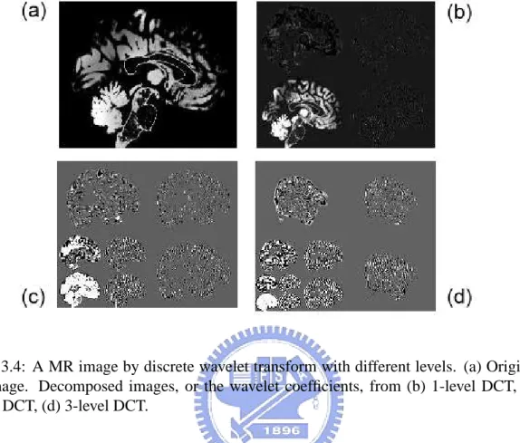
3.4 A MR image by discrete wavelet transform with different levels . . . 42
4.1 The distribution of control points for TPS simulation . . . 48
4.2 The source and simulated images by TPS . . . 50
4.3 Example of a ROC curve . . . 53
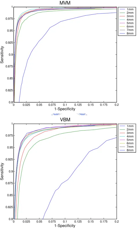
4.4 ROC curves of MVM and VBM results with the simulation data . . . 54
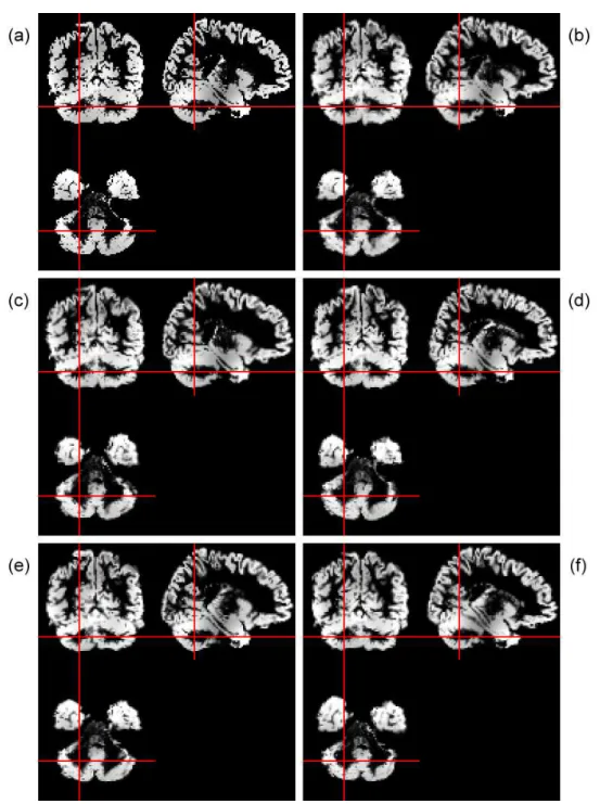
4.5 Analysis result of MVM for 1mm simulated cerebellum atrophy . . . 57
4.6 Analysis result of VBM for 1mm simulated cerebellum atrophy . . . 58
4.10 Analysis result of VBM for 6mm simulated cerebellum atrophy . . . 63 4.11 Strategy for choosing a compatible threshold of MVM by VBMt values . . 67
4.12 Volumetric atrophy of gray matter in SCA3 patients by MVM analysis method . . . 68 4.13 Volumetric atrophy of gray matter in SCA3 patients by VBM analysis method 71 4.14 3-D rendering of GM atrophy in SCA3 by the MVM analysis method . . . 73 4.15 3-D rendering of GM atrophy in SCA3 by the VBM analysis method . . . . 75 4.16 Volumetric atrophy of white matter in SCA3 patients by MVM analysis
method . . . 76 4.17 Volumetric atrophy of white matter in SCA3 patients by VBM analysis
method . . . 77 4.18 Volumetric enlargement of CSF in SCA3 patients by MVM analysis method 80 4.19 Volumetric enlargement of CSF in SCA3 patients by VBM analysis method 81
5.1 ROC curves of MVM results with the non-smoothed and smoothed simu-lation data . . . 88 5.2 How SVM determines the separating hypersurface . . . 90 5.3 Vectors used to obtain a single map for nonlinear classification . . . 92
List of Tables
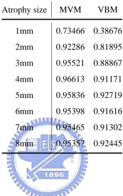
4.1 Definitions of TP, FP, TN, and FN . . . 51 4.2 PAUC indices for ROC curves of MVM and VBM results with the
simula-tion data . . . 55 4.3 Clinical data of patients carrying SCA3 . . . 65 4.4 Atrophy of gray matter in SCA3 patients by MVM analysis method . . . . 69 4.5 Atrophy of gray matter in SCA3 patients by VBM analysis method . . . 72 4.6 Detected GM atrophy of MVM and VBM in SCA3 patients . . . 74 4.7 Atrophy of white matter in SCA3 patients by MVM analysis method . . . . 75 4.8 Atrophy of white matter in SCA3 patients by VBM analysis method . . . . 78 4.9 Detected WM atrophy of MVM and VBM in SCA3 patients . . . 79
5.1 PAUC indices for ROC curves of MVM results with the non-smoothed and smoothed simulation data . . . 89
Chapter 1
In this chapter, we will briefly introduce the human brain structures, the magnetic res-onance imaging (which is an imaging tool often used to detect pathologic tissues from normal tissues), and then the current morphometric methods based on medical images to analyze differennces of brain structures. One of the most popular morphometric approach is the voxel-based morphomety, which have been applied in many researches of brain struc-tures, but it has a inherent defect while detecting subtle and distributed changes. Our goal is to overcome this darwback and to propose a better morphometric method in this work. In the final of the chapter, we will guide the organization of this thesis.
1.1
Brain Structures
Brain is the most sophisticated and elegant organ of human beings. It plays an important role in the control of human mind and behavior. Several involuntary activities, such as heartbeat, respiration, and digestion, and conscious activities, such as thought, reasoning, and abstraction, are all operated by the brain. In the 3rd century B.C., Doctor Herophilus in Alexandria, the ”Father of Anatomy”, is considered as the first person to dissect human body for the purpose of scientific research. He obtained a lot of scientific discoveries, and one of his main contributions is to discover four rooms of the brain, that is, ventricles. Until now, people have done various researches on the brain and understand many the tissues and structures of the human brain.
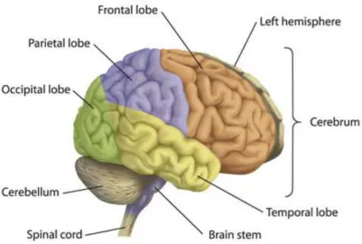
A brain consists of three parts, which are the cerebrum, cerebellum, and brain stem. Brain stem is below the cerebrum and above the spinal cord, and is the major route to con-nect the cerebrum, cerebellum, and spinal cord. Its main function is to maintain individual life, including heartbeat, breath, digestion and the other important physiological faculties. Cerebellum is below the cerebrum and behind the brain stem, and composed of left and right two hemispheres. Cerebellum can balance the body and the posture, and also control the motion of muscle with the cerebral cortex. Cerebrum is considered as the most
impor-1.1 Brain Structures 3
Figure 1.1: Main structures of the human brain. There are three parts, which are the cere-brum, cerebellum, and brain stem. According to sulci and gyri of cerebral hemispheres, brain cortex is divided into four lobes: the frontal lobe, the parietal lobe, the temporal lobe, and the occipital lobe. Photo courtesy of the website of Heart and Stroke Foundation (http://ww2.heartandstroke.ca/).
tant nerve center, and divides into left and right two cerebral hemispheres. Between two cerebral hemispheres is the corpus callosum to communicate left cerebral hemisphere and right cerebral hemisphere. Moreover, according to sulci and gyri of the exterior of cerebral hemispheres, brain cortex can be segmented into four lobes: frontal lobe, parietal lobe, tem-poral lobe, and occipital lobe. The frontal lobe is understood as the central administration of thought. The parietal lobe receives and handles kinds of feeling signals. The temporal lobe has relations with perception and recognition of auditory signals and memory. And the occipital lobe is the center of visual processing. Figure 1.1 shows main structures of the human brain.
According to the type of brain tissues, they can be generally separated into gray matter (GM), white matter (WM), and cerebrospinal fluid (CSF). Gray matter is composed of nerve cell bodies responsible for processing information, and white matter is composed of of the axons responsible for transmissing information. Gray matter forms the exterior part of the brain, and is referred to as the cortex; white matter forms the interior part of the brain,
Figure 1.2: Brodmann’s maps. The human brain is classified into 52 discrete cortical areas in a cytoarchitectonic way. The partitions are referred to as the Brodmann’s areas.
and referred to as the medulla. Cerebrospinal fluid, which is the colorless and transparent fluid, fills ventricles and surrounds the brain and the spinal cord. Cerebrospinal fluid can absorb the shock to the brain or to the spinal cord, and also can drain out waste materials from the brain or from the spinal cord.
In 1909, Brodmann cytoarchitectonically classified brain into 52 discrete cortical areas using a light microscope, and sketched the anatomical maps of the human brain [1]. Each and every area is labeled with a number. Theses are known as the Brodmann’s areas (BAs). Figure 1.2 is the famous Brodmann’s maps. Many BAs were later shown that they are associated to specific functions, such as BA 17 and BA 18 in the occipital lobe (associated to vision). Brodmann’s areas have become a common classification for scientists to refer to
1.2 Magnetic Resonance Imaging 5
a particular region of the brain cortex and the related nervous functions. In 1988, Talairach and Tournoux drew a 3-D stereotaxic atlas and defined the Talairach coordinates of the human brain, by anatomizing the brain of a European female aged 60 [2]. They used Brodmann’s maps as the basis for the architectonic parcellation in their atlas. It is very useful for localization of brain tissues. Thus, when given a 3-D coordinate in Talairach space, we can indicate that which brain structure it is located at and which BA it belongs to, and then know broadly about its associated functions. The Talairach brain is usually taken as the standard stereotaxic space when investigating human brain structures.
Along with progress of science and technology, the first neuroimaging technique, the pneumoencephalography (PEG), was developed in the early 1900s. Invention of the brain imaging technology makes observing the human brain on living beings come true. By these medical images, scientists and doctors can investigate or make a diagnosis about those diseases resulting from some brain disorder as the patients are still alive, rather than dissect patients’ bodies as they were died. Up to now, there are many functional brain imaging technologies, such as positron emission tomography (PET) and single photon emission computed tomography (SPECT); as well as structural imaging technologies, such as X-ray computer tomography (CT) and magnetic resonance imaging (MRI). In this thesis, we used magnetic resonance images as experimental materials to find the structural differences of different brains. In the next section, we will briefly introduce this technology, magnetic resonance imaging.
1.2
Magnetic Resonance Imaging
Magnetic resonance imaging (MRI) is one of popular imaging tools for clinical diagno-sis in recent years. It was developed by Paul Lauterber in 1972 [3]. The technique is based on the principles of nuclear magnetic resonance (NMR) to produce data images of internal physical and chemical characteristics of an object. The original name of this technique
Figure 1.3: A typical MR scanner. Photo courtesy of Lab. of Integrated Brain Research, Department of Research and Education, Taipei Veterans General Hospital.
was nuclear magnetic resonance imaging (NMRI), but people called it magnetic resonance imaging (MRI) because of the word nuclear with the negative connotations of radiation exposure in the late 1970’s.
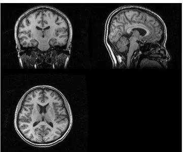
An MR scanner is shown in Figure 1.3. An scanner includes three main hardware de-vices: a main magnet, a magnetic field gradient system, and an RF system [4]. The main magnet generates a strong uniform magnetic field for polarization of nuclear spins in an ob-ject; the magnetic field gradient system produce controlled time-varying gradient fields in different directions to make each of the regions of spin experiences a unique magnetic field for signal localization; the RF (radio frequency) system generates a rotating magnetic field in a pulse sequence to excite spins and detects signals from the spins. All the components of the scanner are placed in a scan room to segregate outside interference. After analysis and reconstruction of signals by a computer, a magnetic resonance image representing the spatial distribution of the inside of living organisms is obtained like Figure 1.4.
MR imaging has many advantages. One is that it is a noninvasive way to detect signals inside the body, so people are unnecessary to bear with pain resulted from invaders of
med-1.2 Magnetic Resonance Imaging 7
Figure 1.4: A 3-D magnetic resonance image of a human head. It is shown in the coronal, sagittal and axial views.
ical treatments. Moreover, this imaging uses magnetic fields and non-ionizing radiation. According to current knowledge, they do not have potential harmful effects to humans. In comparison with some other scanning methods like CT, it is very safe. Another advantage of MR imaging, probably the most important character, is the flexibilty of data acquisition and the outstanding contrast resolution. Therefore, it can be used as spectroscopic imag-ing, diffusion-weight imagimag-ing, angiogarphic imagimag-ing, and functional imaging. That makes MR images able to provide much respectable information and endow the thecnique with superior scientific and dianostic values [4].
Because of the clear contrast resolution, MR images are often used to observe patho-logic tissues from normal tissues, and help doctors to diagnose medical conditions and disorders of the brain. However, such a manual diagnosis is very subjective and time-consuming, especially when the amount of images is large. Thanks to the advances in com-puter, computerized approaches can help to deal with the huge and complex data. Many morphometric analysis methods were proposed to quantitatively analyze MR images by computers.
1.3
Morphometrics
By using MR images, a number of in vivo anatomical studies of the human brain have been done. Most studies are based on the defined regions of interests (ROIs), and then analyze each tissue volumes [5–7] in ROI. However, this method has some limitations. It wastes a lot of time to define the ROIs, especially when there are large amount of subjects [8]. In addition, when analyzing a certain disease, users have to know the most concerned regions [9] before selecting ROIs. It makes ROI-based analysis inconvenient to be used in practice.
Therefore, another kind of automatic morphometric methods, involving the technique of spatial normalization, to characterize neuroanatomical differences has been developed. These methods broadly fall under two categories: (1) ones handle macroscopic differences in shape of brain, and (2) ones handle microscopic differences in brain tissue as the shape differences have been discounted. When connecting these with the technique of spatial nor-malization, the first kind of methods analyzes the parameters or the deformation fields used during the normalization; and the second kind of methods analyzes resulting normalized images after normalization.
The first family of morphometric method includes the pattern-theoretic approach [10], deformation-based method [11, 12], tensor-based method [13, 14], and factor analytic ap-proach [15]. These methods quantify brain shape by using deformation fields obtained from nonlinear registration. This kind of methods can potentially obtain a precise estimation of the brain shape, but it is very sensitive to the accuracy of the underlying normalization approach. Consequently, there are some limitations in practice [9].
The second family of morphometric methods characterizes anatomy in brain tissue by estimating voxel intensities of normalized images. Because this type of methods makes use of images after normalization, the differences in the brain shape are eliminated. Thus, it is
1.4 Motivation 9
suitable for analyzing local and subtle differences in brain tissue. A common-used method, voxel-based morphometry [16], is belong to this family. Besides, the RAVENS [9] is also a kind of these methods.
This thesis emphasizes the second family of morphometric methods. The targeted im-ages are all normalized. Now, the voxel-based morphometry (VBM) is the most popular method applied to analysis of structural brain discrepancy between different groups of im-ages. For each and every voxel from the normalized images, it makes a standard statistical test to examine if there exists a significant difference of brain structure on the location of this voxel. Although VBM is an intuitional and simple approach, it has a fatal defect so that its sensitivity to some kind of group differences is bad. Our goal is to propose a method to ameliorate this lack. In the following, we will briefly indicate the main drawbacks of the VBM analysis, and try to improve according to the fundamental cause of it. It goes into details in chapter 2.
1.4
Motivation
Although VBM is one of most popular morphometric method and has been applied successfully in many instances, there are still limitations that make VBM disable to detect particular anatomical differences in some situations. These limitations are caused by the inherent defect of this approach. It is because VBM is a voxel-by-voxel manner, i.e. a univariate method, to analysis differences by using standard statistical tests at each distinct voxel. That means when VBM tests group difference at a particular voxel, it only takes measurements of images at this voxel in account at a time, and discards potential informa-tion carried by other voxels adjacent to this voxel. The way of VBM to analyze the brain structures makes this method simple to use. However, from the spatial point of view, such the voxel-wise manner to find anatomical differences appears improper, because it treats each voxel as an independent object. Adjacent brain tissues should have relations to each
other. As a result, this method is criticized for its capability to estimate widely-distributed, continuous and subtle changes in brain structure [17].
In this work, we proposed a novel method that can consider interrelations between voxels, called the multivariate volumetric morphometry (MVM). In this method, a high-dimensional classification technology is employed. It seeks the most discriminative hyper-plane that separates populations by minimizing the scatter within each individual group and simultaneously maximizing the scatter between groups. The discriminative hyper-plane not only has the ability to classify different groups, but also is appropriate to be used in this application of characterizing the anatomical group discrepancy. Besides, before using this classification technique to find brain differences, a recombination of the spatial and frequency signals is performed for the multiresolution analysis. Our method is built on the classification and the data recombination techniques.
In this thesis, we not only demonstrate the effectiveness of the proposed method, but also develop an efficient computational implementation to save time for analysis. More-over, a part of idea of this method has been proved in this work. Experimental results showed that the multivariate volumetric morphometry (MVM) indeed has a better sensitiv-ity to subtle and distributed changes of brain structures. So, it is very useful to characterize early symptoms of a disease especially. The details of the reason why we need a multivari-ate approach and the proposed method are described in the chapter 2 and 3, respectively.
In the following chapters, we introduce the voxel-based morphometry and its drawbacks in chapter 2, and then our method in chapter 3. In chapter 4, some experiments are used to estimate the accuracy of the proposed method, and the comparison between the results of MVM and VBM is performed. Finally, we will bring up some issues about our method MVM in chapter 5, and conclude this work in chapter 6.
Chapter 2
This chapter is about one of the most popular morphometry—the voxel-based mor-phometry (VBM). After the introduction, there is a brief interpretation of the basic concept and the optimized protocol of VBM. In the end of this chapter, we statement the inherent drawback of such a voxel-based morphometric analysis, and that is the motive for us to develop another method characterizing anatomical differences.
2.1
Introduction to VBM
The voxel-based morphometry (VBM) is a technique measuring concentrative or volu-metric group differences of brain tissues through a voxel-wise analysis of MR images [16]. It is an unbiased and objective method, which explores whole brains rather than specific regions to find the significant structural discrepancy between different groups of subjects. That means people can use the method without the need for the background knowledge of where the discrepancy may exist.
Due to its simplicity, feasibility, and effectiveness, VBM has been widely applied to structural brain studies in the recent years. It is shown in earlier researches that many dis-eases are related to the abnormal brain structures. The defect, damage, or irregularity of the brain structure will cause irregular behavior of patients. Several studies using VBM characterizing brain differences in a certain disease had good outcomes consistent with observations of those previous researches, such as schizophrenia [18–20], Alzheimer’s dis-ease (AD) [21–23], autism [24,25], spinocerebellar ataxia (SCA) [26], and attention deficit hyperactivity disorder (ADHD) [27].
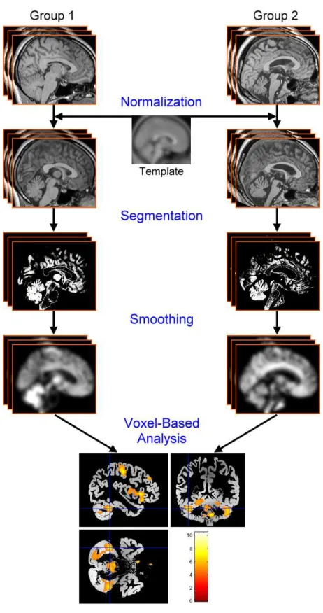
VBM includes a preprocessing and a voxel-based parametric statistical analysis. Basi-cally, the preprocessing involves spatial normalization, segmentation, and smoothing [16]. The spatial normalization is responsible for registering brain images of different subjects into the same stereotactic space defined by a template image. In the space, we assume
2.1 Introduction to VBM 13
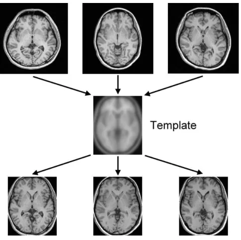
Figure 2.1: The normalization. Images in the upper row, the middle row and the lower row are native MR images, template image and normalized images respectively. Before normalization, the scales and shapes of heads of different subjects are dissimilar. Normal-izing images with a standard brain template makes all images in the same stereotactic space where the voxel-wise comparison can be preformed.
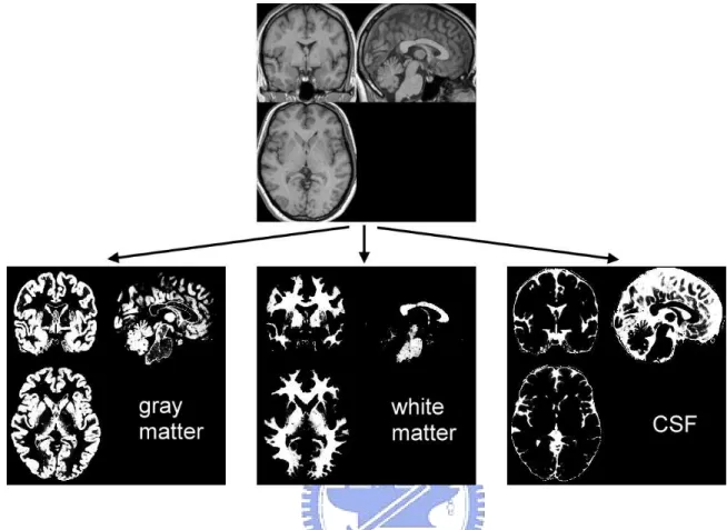
Figure 2.2: The segmentation. The figure shows segmentation of a normalized image into different tissue classes. The resulting segments includes a gray matter (GM) image, a white matter (WM) image, and a cerebrospinal fluid (CSF) image.
that measurements of one certain voxel in different normal brain images should represent the same brain tissue. In the segmentation, the images are segmented into different tis-sue classes as the gray matter (GM), white matter (WM) or cerebrospinal fluid (CSF). That makes statistical analysis can be performed on different brain tissues. The smoothing is necessary for the following statistical analysis. It conditions the data more normally-distributed and reduces the registration error resulted from the normalization, to increase the validity of inferences based on parametric tests. Figure 2.1 and Figure 2.2 illustrate the concept of normalization and segmentation respectively. After preprocessing, the voxel-based statistical analysis is performed by comparing the normalized and smoothed GM or/and WM images of different groups of subjects. That is, it uses a standard (univariate)
2.2 Optimized VBM Protocol 15
statistical test with a null hypothesis at each and every voxel, to evaluate whether the voxel values of different groups reach the significant level in statistic. If reaching the significant level, we can say there is a difference between the groups at this position of this voxel. The resulting statistical parameters are assembled into an image. Finally, voxels with the statistical parameters preceding the significant level form the regions representative of the detected group differences.
The following is the summary of basic VBM steps [16], and its corresponded flowchart is shown in Figure 2.3:
1. Spatially normalization of all images to the same stereotactic space
2. Segmentation of normalized images into GM, WM, and CSF
3. Smoothing
4. Voxel-based statistical analysis
5. Making inferences about group differences
Actually, there are various methodological implementations of voxel-based morphome-tric analysis. For example, the RAVENS [9] applied segmentation first, and then normal-ization, smoothing and statistical analysis. In next section we will introduce one of the most popular the implementations—the optimized VBM protocol [28]. It was used and compared to our mehtod in this thesis.
2.2
Optimized VBM Protocol
There are several cases that some structural differences found by VBM do not really exist between groups of subjects when using the basic VBM steps. The misinterpreted
2.2 Optimized VBM Protocol 17
differences may be resulted from bad results of normalization which induce subsequently inappropriate comparison between dissimilar brain structures [29]. Although missegmen-tation leads to the incorrect comparison seemingly, in fact, missegmented tissues are often caused from badly normalized images. It is because in the implement of segmentation of normalized images into gray matter, white matter and cerebrospinal fluid (CSF), Ash-burner and Friston use a mixture model cluster analysis designating the distributions of voxel intensity of specific tissue types, and use a priori probability maps describing a priori knowledge of the distribution of different brain tissues in normalized normal subjects to accomplish tissue segmentation [16]. Notice that the a priori probability maps are in the normalized stereotactic space. The efficiency of segmentation is influenced by effect of normalization, because better normalization makes a priori knowledge of the brain tissue distribution can be used more validly in the segmentation. Thus, to minimize the probability of inappropriate comparison between dissimilar brain tissues and structures is to minimize potential error of normalization. For the reason, when wanting to measure group differ-ences of GM/WM, normalization is preformed on the segmented GM/WM images rather than on the whole brain images to increase correctness of GM/WM registration results. If the GM/WM images used for normalization are well segmented, then normalization will most likely be fine. It becomes interesting that, a good outcome of normalization could lead to a good outcome of segmentation, and vice versa. Accordingly, the optimized VBM protocol proposed by Good et al. [28] adopts an iterative version of segmentation and nor-malization to improve effects of preprocessing.
The following is the optimized VBM protocol for measuring group differences of gray matter [28], and its flow diagram is shown in Figure 2.4:
1. Creation of customized T1 template and a prior probability maps of GM, WM
and CSF
Customized template is used to reduce potential bias which results from the scanner and the subject population differing from the existing template. All brain images are
Smooth GM image Modulation Modulated GM image Smooth Segmentation & extraction GM/WM/CSF priors T1 template Normalized T1 image Apply deformations Deformation filed Spatial normalization GM image Segmentation & extraction Affined T1 image Affine registration GM prior Statistics (volumes) Statistics (concentrations) T1 image Smooth GM image Modulation Modulated GM image Smooth Segmentation & extraction GM/WM/CSF priors T1 template Normalized T1 image Apply deformations Deformation filed Spatial normalization GM image Segmentation & extraction Affined T1 image Affine registration GM prior Statistics (volumes) Statistics (concentrations) T1 image
Figure 2.4: Flowchart of the preprocessing of optimized VBM protocol for estimating brain discrepancy of gray matter. It is executed in order of (1) creation of customized T1 template and a prior probability maps of GM, WM and CSF, (2) segmentation and extraction of affine-registered whole brain images, (3) obtaining optimized normalization parameters by normalizing GM images into GM template, (4) normalization of whole brain T1 images with optimized normalization parameters, (5) segmentation and extraction of normalized whole brain images, (6) modulation (if need), and (7) smoothing.
2.2 Optimized VBM Protocol 19
first normalized to the ICBM 152 template (Montreal Neurological Institute), and then segmented into different brain tissues as gray matter, white matter and CSF. Fi-nally, the normalized T1, gray matter, white matter and CSF images are smoothed with an 8mm FWHM isotropic Gaussian kernel and then averaged to create the cus-tomized T1/gray/white/CSF mean images (template and priors).
2. Segmentation and extraction of affine-registered whole brain images
In the step, all original structural MR images are affine-registered to the customized T1 template and then segmented with the GM/WM/CSF a prior probability maps derived from above step in native space, followed by morphological operations to remove unconnected non-brain tissues of segmented images. Notice that there is a caveat that the segmentation is preformed in native space, but the a priori probabil-ity maps are in the normalized stereotactic space. Therefore, there will be another segmentation of normalized images in the following to produce better segmented images.
3. Obtaining optimized normalization parameters by normalizing GM images into
GM template
To obtaining the optimized normalization parameters, segmented gray matter images are normalized to the customized gray matter template, which is the GM a prior probability map derived from the first step, by applying 12-parameter affine trans-formation and nonlinear spatial warping using discrete cosine basis functions. As a result of normalization of gray matter images rather than whole brain images, the normalization parameters of gray matter are optimized by preventing any deforma-tion contribudeforma-tions of non-GM tissues. When wanting to measure group differences in white matter instead, we obtain the optimized normalization parameters just by normalizing WM images into the WM template.
4. Normalization of whole brain T1 images with optimized normalization
All original MR images then are normalized with the optimized normalization pa-rameters. The resolution of normalized images should be relatively high for reduc-ing partial volume effects, which means there is a mixture of different tissue types at one voxel and confounds the subsequent tissue segmentation. In common cases, the voxel size of the normalized image is isotropic in three dimensions.
5. Segmentation and extraction of normalized whole brain images
This step involved segmentation of optimally-normalized images. The images are divided into gray matter, white matter and CSF partitions in the normalized stereo-tactic space. Non-brain tissues are removed by using morphological operations and a brain mask. In addition, this step also incorporates a correction of image intensity nonuniformity [16] which is mainly caused by magnetic field inhomogeneity of the RF coils during image acquisition. The resulting images are extracted gray matter partition. When estimating WM group differences, extracted WM images are the ticket.
6. Correction for volume changes (optional)
In the segmented image, the value of each voxel is assigned the a posteriori proba-bility that the voxel is classified into this particular tissue type, ranging between 0 and 1. Thus, the segmented GM/WM/CSF data will represent the concentration of GM/WM/CSF. To preserve the total amount of brain tissue, a correction for volume changes, which is usually referred to as “modulation”, is performed by multiplying a voxel value by its Jacobian determinant, which is the relative volume before and after normalization (in step 4). After this correction, these modulated images rep-resent the volume of brain tissues. And, to analyze the modulated images is to test group structural differences in the absolute amount of brain tissues. In this thesis, we always used modulated data to estimate volumetric group differences rather than used non-modulated images to consider the differences in concentration.
2.2 Optimized VBM Protocol 21
The normalized, segmented, and modulated images are smoothed with a Gaussian kernel in this step. Smoothing is necessary for the following voxel-based paramet-ric tests. It substitutes the value of each of voxels with a weighted average of sur-rounding voxels. By the central limit theorem, this action conditions the data more normally distributed such that the validity of inferences based on statistical tests can be increased. Smoothing also reduces the registration error of spatial normalization. However, it is worth noticing that, the choice of the smoothing kernel size should be corresponding to the size of the expected regional differences [30]. Many studies adopt an 8-mm or 12-mm FWHM smoothing kernel when using the VBM method.
8. Statistical analysis
After the preprocessing, the final step is a voxel-wise statistical analysis of normal-ized and smoothed gray matter images. Statistical analysis employs the general lin-ear model, which is a flexible framework allowing many different tests to be applied, to distinguish significant differences in brain structures of different groups under study [31]. In this thesis, we applied two-sample t-test as the fitting model to
de-scribe data of two groups, and used the standard (univariate) parametric t tests to
evaluate the residuals at each and every voxel. The resulting statistical parameters of
t tests are assembled into an image called the t-test map. By setting a significance
level and a minimum cluster size to the t-test map, voxels with the statistical
pa-rameters preceding the significant level and in the clusters whose size is larger than the minimum cluster size form the regions representative of the detected significant group differences.
In this work, we not only applied the optimized voxel-based morphometry to compare the capability of revealing structural brain discrepancy between different groups with one of our method, but also used the preprocessing of the optimized VBM protocol to deal with MR images before analyzing them by the proposed method. That is, the implementation of this image preprocessing was also applied in our method. Here we used the SPM2
Voxel 1
Voxel 2
Voxel 3
…
Voxel N
x = (x
1, x
2, x
3, … ,x
N)
Figure 2.5: Concept of a MR image lying in a high-dimensional space. x represents a image withN voxels. If we rearranged voxels of the 3-D image to produce an unique 1-D
vector by a particular fixed order, then x can be regarded as one point in aN -dimensional
space, where each dimensioni stands for voxel i, for i = 1, . . . , N .
software (the Wellcome Department of Imaging Neuroscience, University College London, UK) implemented in Matlab 6.5 (the MathWorks, Inc. Natick, MA, USA) to accomplish all procedures involved in the optimized voxel-based morphometry.
2.3
Drawbacks of VBM
Since an individual MR image, a kind of morphological profiles, is commonly de-scribed as a collection of voxel-wise morphological measurements, it can be placed in a high-dimensional space where each dimension presenting a voxel. That is, a MR image is thought as one sample point in a high-dimensional space whose dimensionality is equal to the number of voxels of the MR image. Figure 2.5 graphically illustrates this concept. When all images have the same sizes and have been normalized into the same stereotactic space, where voxels at the same position in all the images should contain the same brain tissue, the patient morphological profiles and the normal morphological profiles will form two distributions in the high-dimensional space, like Figure 2.6 shows.
2.3 Drawbacks of VBM 23 Voxel 1 Voxel 2 (b) Voxel 1 Voxel 2 (a)
Figure 2.6: Schematic illustration of the significant bias of VBM. Each ellipse represents a population of one group. In the case of (a), we can see that the group discrepancy almost centralizes at the position of voxel 1, so it is very probable that VBM detects a difference at voxel 1 but has no finding at voxel 2. In contrast, because the group discrepancy is spread at voxel 1 and voxel 2 in the case of (b), the difference at voxel 1 and voxel 2 is obscure. Therefore, the voxel-based morphometry may fail to find any differences, even though the discrepancy between the two groups has the same overall magnitude with case (a). These simple two cases show the instability that, the ability of VBM to detect group discrepancy is influenced by the distribution, or pattern, of the discrepancy.
However, Davatzikos [17] pointed out that there is a significant bias of VBM to ren-der inferences about group differences. Let consiren-der two cases where the morphological differences between two groups have the same overall magnitudes in Figure 2.6 (a) and (b). For the purpose of display, there are only two dimensions in the figure, but the di-mensionality is much higher in practice. Because voxel-based morphometry detect group differences voxel-by-voxel, only the values along one dimension are taken into account at a time. In the Figure 2.6 (a), there is a significant group difference at the voxel 1, since the two distributions along voxel 1 are easily separated. It is probable that VBM can detect a difference at voxel 1. Along the voxel 2, the situation is opposite, thus VBM may fail to find any difference at voxel 2. Now we focus on the case in the Figure 2.6 (b). It is clear that there is a group discrepancy spreading at voxel 1 and voxel 2. But in the voxel respect, a large overlap of distributions of two groups exists along both voxel 1 and voxel
2. This situation may cause VBM disable to detect any differences at either voxel. This simple example in Figure 2.6 (b) reveals that when applying voxel-based morphometry to estimate group discrepancy, some subtle and complex patterns of brain differences, which are widely distributed over many voxels, may not be significant at each single voxel for VBM to detect.
From the cases in Figure 2.6, we know there is a bias in VBM that, it detects relatively localized differences much easier than relatively distributed differences involved with sev-eral brain structures [17]. This bias is an unavoidable and fatal problem to VBM, and it makes the analysis result of VBM forced to be relied upon the disease characteristics. The problem results from that VBM analyzes the group discrepancy in a voxel-by-voxel manner rather than considers the entirety of voxels simultaneously. In such the voxel-wise analysis method, related information carried by the neighboring voxels are not considered, so it may cause the disability to measure the subtle and widely-distributed discrepancy located in a large region composed of many voxels. Therefore, we proposed another unbiased and au-tomatic method, using a multivariate analysis approach, called the multivariate volumetric morphometry (MVM) to break this limitation of univariate analysis.
Chapter 3
Owing to the congenital problem of this voxel-wise comparison approach, in this chap-ter we will introduce the proposed method called the multivariate volumetric morphometry (MVM) which can assess anatomical brain differences. The MVM includes a preprocess-ing and an analysis step as VBM does. The image preprocesspreprocess-ing of MVM is the same with one of VBM (shown in Figure 2.4), in which the modulation is required to charac-terize volumetric group differences of brain tissues, but the data smoothing is omitted. In the statistical analysis step, MVM adopts a reformatory LDA-based method as the basis of multivariate analysis, and conjugates the wavelet transform, which is used to rearrange the spatial and frequency information for the multiresolution analysis, to measuring group differences. Because each and every voxel represents one variate in analysis, thus MVM is a multivariate approach. This method overcomes the drawback of voxel-based analysis, and is appropriate for estimating the structural brain discrepancy between different groups.
3.1
Ideas of the Proposed Method
The multivariate volumetric morphometry (MVM) is the proposed method which char-acterizes volumetric anatomical discrepancy between different groups through a multivari-ate analysis of MR images of particular brain tissues. It is an unbiased, objective and whole-brain measurement. The multivariate volumetric morphometry contains several pro-cesses like VBM does, and the chief breakthrough of this thesis is the multivariate analysis. Thus, in the following, we only focus on the statistical analysis step of MVM.
In the multivariate analysis stage, it employs a high-dimensional classification tech-nique, which considers all voxels of MR images at one time, to identify the most discrim-inative hyper-plane that well separates the populations of groups in the high-dimensional space. This hyper-plane goes along with a unique normal vector, the most discriminant pro-jection vector w, which is the direction shifted from one population to another population. The appearance of a shift might be resulted from some factors of interest cause the group
3.1 Ideas of the Proposed Method 27
Voxel 1
Voxel 2
w
Figure 3.1: Sketchily showing how a high-dimensional classification technique can be used to measure group differences. Assume the yellow points are the patients’ morphological profiles, and the corresponding yellow elliptic area is the patients’ distribution; either are the blue ones for normal subjects. A classification technique determines the most discrim-inative hyper-plane, which is presented by the dotted line, and the corresponding most discriminant projection vector w. In such the projection vector w, each element denotes the discrimination weight of group discrepancy. Therefore, the vector w can be considered as a spatial map containing the regions representative of group differences.
discrepancy under study. The most discriminant projection vector is also an image which has the same size of all sample images. The way of using a classification technique to find such the most discriminant projection vector does not need to coincide along any voxels (di-mensions), that voxel-based analyses are unable to achieve. Further, each of the parameters from the most discriminant projection vector w denotes the weighting, or the discrimina-tion of characterizing group discrepancy, so the most discriminant projecdiscrimina-tion vector can regarded as the analytic image containing the resulting analysis parameters. In this way, we can quantify differences throughout the whole brain between different groups by such a high-dimensional classification technique. Figure 3.1 illustrates the idea schematically.
3.2
Framework of Multivariate Volumetric Morphometry
Before the multivariate analysis, we used the first six steps of the optimized VBM pro-tocol mentioned in the chapter 2 to obtain individual normalized and modulated gray/white matter images. Notice that the smoothing was disused. The reason why we do not smooth the images in the multivariate volumetric morphometry will be explained in chapter 5, discussion. Then, in the central multivariate method, we used a reformatory LDA-based method, the discriminative common vector method [32], to find the most discriminant pro-jection vector which minimizes the scatter within each individual group and simultaneously maximizes the scatter between groups without the small sample size problem. The result-ing projection vector forms a spatial map, whose image size is the same with all gray/white matter images used for the analysis, containing the regions which are most representative of group differences. The details of the method and its efficient implementation we proposed for implementation will be interpreted in the next section.
Besides the discriminative common vector method, we also used the wavelet transform rearranging the spatial and frequency information of MR images to improve the effect of MVM upon catching significant group differences, in several varied scales. The reason we applied the discriminative common vector method in the wavelet space is that, although the method considers all voxels of images simultaneously when estimating group differ-ences, there are the same forces of relationships between all pairs of two voxels in the method; no matter the two voxels are adjacent to or far away from each other. Thus, to increase spatial correlations between neighboring voxels, the 3-D wavelet transformation is used to restructure voxel data into space-scale features in a hierarchical representation way. After that, we then apply the discriminative common vector method on these wavelet features. Moreover, the wavelet transform also makes the analysis become a multivariate multiresolution analysis.
3.2 Framework of Multivariate Volumetric Morphometry 29
of each feature from the projection vector represents the degree of importance for charac-terizing the group differences. The number of features, equal to the number of voxels in a MR image, is usually a huge amount. Only the features with larger weights in the most discriminant projection vector are used when performing the inverse 3-D wavelet transfor-mation, to obtain the final discriminating map in the original voxel-based space. Discarding the features with small weights helps to remove trifling differences and to improve accuracy of the multivariate analysis.
Finally, for the purpose of determining and displaying which regions representative of the significant group differences, a smoothing and thresholding of discrimination weights of the parameters in the discriminating map are needed. As mention before, each parameter of the discriminating map denotes the discrimination of characterizing the group discrep-ancy, so in an intuitively thinking, the changes of the weights of neighboring parameters should be slight. However, in practice, it does not often look smooth as we think. It may result from the noise or the variation within groups, or the error produced during the pre-processing like a wrong image registration or tissue segmentation. It happens especially when we abandon the smoothing step in MVM preprocessing. Therefore, to constrain the smoothness of discrimination weights in the discriminating map regionally, we use a smoothing for the discriminating map. In addition, a thresholding is done before displaying the discriminating map to show the detected regions most representative of group discrep-ancy. Only voxels with a parameter value preceding the threshold in the discriminating map are considered to reach the significant level and to shall be showed. The minimum cluster size of the parameters also can be set to reject the too small regions. Although the smoothing and thresholding are not the parts of the multivariate analysis step, they are need for visualizing the discrepancy pattern between the groups. Of course, both of the procedures can be regulated by users. In the end of the MVM analysis, we can also obtain a whole-brain confidence in explaining whether the detected group discrepancy is correct, by caculating the p-value associated with the T-statistic on the two groups of projected
images onto the discriminating map.
Summarily, the multivariate volumetric morphometry (MVM) contains the following steps:
1. Spatially normalization of all images to the same stereotactic space
2. Segmentation of normalized images into GM, WM, and CSF
3. Correction for volume changes of segmented images
4. Multivariate analysis
(a) Forward 3-D wavelet transformation to the multiresolution space
(b) Discriminative common vector method to obtain the most discriminant projec-tion vector
(c) Discarding unimportant wavelet features with small discrimination weights in the most discriminant projection vector
(d) Inverse 3-D wavelet transformation to obtain the discriminating map in the stereotactic normalization space
5. Visualization of the discrepancy pattern
(a) Smoothing (b) Thresholding
Figure 3.2 is the flowchart of the multivariate analysis part of MVM. In implementation, we used the first six steps of the optimized VBM protocol to accomplish the step 1 and 2 of MVM. In the following sections we will introduce the techniques used in the mul-tivariate analysis step, including the discriminative common vector method, the efficient implementation for the discriminative common vector, and the 3-D wavelet transform.
3.2 Framework of Multivariate Volumetric Morphometry 31
3.3
Multivariate Analysis using a Reformatory LDA-Based
Method
3.3.1
Conventional Linear Discriminant Analysis and Its Potential
Prob-lem
The linear discriminant analysis (LDA) is one of the most popular linear projection techniques. It was invented by Ronald A. Fisher in 1936 [33], and has been successfully applied in many classification problems such as image recognition, multimedia informa-tion retrieval and so on. Its goal is to find the most discriminant projecinforma-tion vector w, in which direction groups can be separated with the maximum between-class scatter and the minimum within-class scatter.
LetK be the number of classes (groups), where the kth class contains Mksamples, and
let xkmbe aN -dimensional column vector which denotes the mth sample of the kth class.
There is a total ofM = PKk=1Mk samples. The within-class scatter matrix Sw and the
between-class scatter matrix Sb are defined as
Sw = K X k=1 Mk X m=1 (xk m− µ k)(xk m− µ k)T, (3.1) and Sb = K X k=1 Mk(µk− µ)(µk− µ)T, (3.2) whereµk = 1/M kPM k
m=1xkm as the mean of samples in thekth class, and
µ = 1/MPKk=1PMk
m=1x k
m as the mean of all samples. The objective of LDA is to find a
projection matrix Plda that maximizes the Fisher’s linear discriminant criterion, that is
Plda = arg maxP F (P) = arg maxP
|PT
SbP|
|PTSwP|. (3.3)
According to linear algebra, the ratio is maximized when the column vectors of Plda are the eigenvectors of S−1w Sb. In implementation, each individual morphological profile is
3.3 Multivariate Analysis using a Reformatory LDA-Based Method 33
first reshaped into a sample vector by arranging the 3-D volume in some consistent order before applying the linear discriminant analysis. Moreover, there are only two groups in our case, i.e. K = 2, so we can immediately obtain the most discriminant projection vector
w, which is the only one eigenvector composing Plda, by the formula w = S−1w (µ1− µ2).
However, LDA encounters difficulties when the number of samples is much smaller than the dimensionality of the sample space. This situation causes the within-class scatter matrix singular and not invertible, so the LDA cannot be applied directly. It is known as the small sample size (SSS) problem [34]. Therefore, we employ the discriminative common vector method [32], which was proposed by Cevikalp and Wilkes for face recognition, to solve this problem.
3.3.2
Discriminative Common Vector Method
The discriminative common vector method for the small sample size problem is based on a variation of the LDA by maximizing the modified Fisher’s linear discriminant criterion [35]. The general idea of the common vector is to find a vector which can represent a class by extracting common properties of the class, or saying that, by eliminating differences between the samples in the class. After getting each common vector of every class, we can use the principal components analysis (PCA) [36] to find the principal components which actually equate the most discriminant projection vectors of LDA.
Let us use all previous definitions and let the total scatter matrix be defined as
St = K X k=1 Mk X m=1 (xk m− µ)(x k m− µ) T = Sw + Sb. (3.4)
The modified Fisher’s linear discriminant criterion
ˆ F (P) = |P T SbP| |PTStP| = |PT SbP| |PTSwP + PTSbP| (3.5)
has been proved that it is exactly equivalent to the original Fisher’s criterion by Liu et al. [35], saying that
arg max
P
ˆ
F (P) = arg max
P F (P). (3.6)
The modified criterion will attain a maximum in the special case, proved in [37], where
pTSwp = 0 and pTSbp 6= 0, for all projection vectors p ∈ RN \ {0}. Under these
conditions for p, a better criterion [38] will be
arg max |PTS wP|=0|P T SbP| = arg max |PTS wP|=0|P T StP|.
That is to say, if we transform all samples onto the null space of Sw to restrict the projected within-class scatter matrix to be a zero matrix, and then calculate the principal components that maximize |PT
StP| by performing PCA, we will obtain the most discriminant
pro-jection vectors without the small sample size problem. It is called the null space method proposed by Chen et al. [37].
The transformation matrix from the original sample space to the null space of Sw is
¯
Q ¯QT, where the column vectors of ¯Q are the vectors spanning the null space of Sw. Cevikalp and Wilkes [32] have proved that, projecting every samples xkm (which denotes
the mth sample of the kth class) in the kth class onto the null space of Sw will produce
exactly one vector xkcom = Q ¯¯QTxk
m , which is referred to the common vector; moreover,
because of ¯Q ¯QTxk
m = xkm− QQ Txk
m, the common vector xkcom of the kth class can be
calculated without ¯Q by using
xkcom = xkm− QQTxkm, (3.7) where Q is the matrix whose column vectors are the orthonormal vectors spanning the range space of Sw. Since the number of columns in Q is about M and the number of columns in ¯Q is aboutN − M, the size of Q is much smaller than the size of ¯Q. It states
that the method can greatly reduce the computational burden than the null space method.
After obtaining the common vector for each and every group, the principal components of those common vectors will be the most discriminant projection vectors. It is because
3.3 Multivariate Analysis using a Reformatory LDA-Based Method 35
there is exactly one class over the common vectors now. These principal components of the common vectors are called the discriminative common vectors. Again, in our practice, samples are divided into only two groups, so there is only one discriminative common vec-tor in the event. We obtain the most discriminant projection vecvec-tor w by directly subtracting of the two common vectors, namely, w= x1
com − x2com.
So the steps of the discriminative common vector method are as follows:
1. Compute the eigenvectorsα1, α2, . . . , αrcorresponded to the nonzero eigenvalues of
Sw, where r is the rank of Sw, and set Q = [α1 α2 · · · αr].
2. Obtain the common vectors for each class by choosing any sample from each class and projecting it onto the null space of Sw, those are
x1com = x1m− QQTx1m, m ∈ {1, . . . , M1}, (3.8)
and
x2com = x2m− QQTx2m, m ∈ {1, . . . , M2}. (3.9)
3. Compute the only one discriminative common vector, i.e. the most discriminant projection vector w by
w= x1
com − x2com. (3.10)
3.3.3
Efficient Implementation for Computing Discriminative
Com-mon Vectors
Although the discriminative common vector method solves the small sample size prob-lem, there are still come difficulties in implementation. It is because the dimensionality of the sample space is a very huge amount. For example, a 3-D image with the size
157 × 189 × 156 has more than 4.6 × 10⁶
voxels. Therefore, we proposed an efficient implementation for computing the discriminative common vector.
Since the within-class scatter matrix is defined as Sw =PKk=1 PMk m=1(x k m− µk)(xkm− µk)T, it can be rewrited as Sw = AAT, (3.11)
where the matrix A = [x1 1 − µ 1 · · · x1 M1 − µ 1 x2 1 − µ 2 · · · x2 M2 − µ 2 ]. Rather
than directly calculating the large N -by-N matrix Sw, we used a computationally fea-sible method [39, 40] to compute the eigenvectors of AAT by multiplying the matrix A by the matrix ˜Q whose columns are the eigenvectors of ATA. So the matrix representation of
the subsequent operations is written as
Q = A ˜Q x1com = x11− Q(Q Tx1 1) x2com = x21− Q(Q Tx2 1) w = x1 com − x2com, (3.12)
where we choose the first sample of each class to obtain the common vector.
However, there is still a heavy computational cost if we translate these equations into programming codes without simplifying them. It is known that, a matrix multiplication
BC needsn1× n2× n3multiplications when the matrix B isn1-by-n2and the matrix C is
n2-by-n3. So, how many multiplications it will take if we do not change the computation
way? For this purpose, we developed an efficient implementation to achieve the above objective (3.12). The following is the pseudo-code:
1 forj := 1 to r do
2 fori := 1 to N do
3 qj(i) := 0
4 forl := 1 to M do
5 qj(i) := qj(i) + A(i, l) ∗ ˜Q(l, j)
3.3 Multivariate Analysis using a Reformatory LDA-Based Method 37
7 end
8 qj := N ormalizeV ector(qj)
9 dot1 := Dot2V ectors(qj, x
1 1)
10 dot2 := Dot2V ectors(qj, x
2 1)
11 fori := 1 to N do
12 QQtX1(i) := QQtX1(i) + qj(i) ∗ dot1
13 QQtX2(i) := QQtX2(i) + qj(i) ∗ dot2
14 end 15 end 16 fori := 1 to N do 17 w(i) := (x1 1(i) − QQtX1(i)) + (x 2 1(i) − QQtX2(i)) 18 end
In this code fragment, the scalarsr, N , M are the number of column vectors composed
of ˜Q, the dimensionality of the sample space, and the number of all samples, respectively.
The vector qj represents the jth column vector of Q. The N -by-M matrix A and the
M -by-r matrix ˜Q represent as the definitions before. And, the vector QQtXk, used to
calculate the common vector xkcom, represents the projected sample of xk1 of the range
space of Sw, for k = 1, 2. Furthermore, the function N ormalizeV ector() makes the input vector turning out a vector with the norm equal to 1 in the same direction. The function Dot2V ectors() returns the scalar product of the input vectors. Finally, the resulting vector w is the most discriminant projection vector.
3.4
Multiresolution Analysis using Wavelet Transform
In image processing, there are many methods and theories to be developed. Owing to convenience of analysis, it usually transforms domain of signals. In engineering applica-tion, the most popular method is Fourier transform. Fourier transform can transform the signals from spatial domain to frequency domain, but the information of spatial domain is lost after applying Fourier Transform on an image. In many applications, however, it needs to analyze both frequency and spatial information at the same time. To avoid the lack of spatial information, Haar, Goupillaud, Grossman, and Morlet proposed and improved wavelet transform [41].
Wavelet transform is one of multi-resolution analysis. Wavelet transform not only can transform an image from spatial domain to frequency domain, but also has information of both two domains. Similar to the Fourier transform, wavelet transform consists of ous wavelet transform (CWT), and discrete wavelet transform (DWT). However, continu-ous wavelet transform is limited by the redundancy and impracticality in image processing. Therefore, the discrete wavelet transform is applied in this thesis.
3.4.1
3-D Discrete Wavelet Transform
The most important parameter in wavelet transform is called wavelet function, which is also called mother wavelet. Wavelet functionψ(x), where x is the parameter in the spatial
domain, has to satisfy two properties as follows:
1. The integration of wavelet function has to be zero,
Z ∞
−∞
3.4 Multiresolution Analysis using Wavelet Transform 39
2. Wavelet function has finite energy,
Z ∞
−∞|ψ(x)dx|
2
< 0. (3.14)
First property represents that wavelet function is oscillating, so wave function is always like an oscillatory wave. Second property represents finite energy, so wavelet function decays to zero in both positive and negative directions. Compared with harmonic waveform, wavelet function is relative smaller. This is the underlying reason that it is called ”wave-let”.
In this thesis, wavelet transform is used for the multiresolution analysis. Wavelet trans-form based multiresolution analysis is to analyze the signals or images under different scales and resolutions. Utilizing the multiresolution analysis, an image with complex fre-quencies can be decomposed into many images with simple frefre-quencies. The decomposed images can be analyzed independently or in community. To discuss the method of multi-resolution analysis, besides wavelet functions, the scaling functions, usually inferred to the father wavelet, have to be introduced. Define the scaling function φ(x), which have to
satisfy three basic properties:
1. The integration of scaling function has to be 1,
Z ∞
−∞
φ(x)dx = 1. (3.15)
2. The energy of scaling function is equal to 1,
Z ∞
−∞|φ(x)dx|
2
= 1. (3.16)
3. The scaling functionφ(x) and its transformation by shifting n, φ(x − n), compose of an orthogonal set,
< φ(x), φ(x − n) >= δ(n), (3.17)
where δ(n) is Kronecker delta symbol. δ(n) = 1 as n = 0, and δ(n) = 0 as n 6= 0. Wavelets can be defined by the wavelet function and the scaling function. Moreover, the