Person-fit偵測作假之效用- 非參數試題反應理論的模擬與應用 - 政大學術集成

全文

(1)國立政治大學教育學系教育心理與輔導組博士論文 . 指導教授：余民寧博士 . Person-fit 偵測作假之效用‐ 非參數試題反應理論的模擬與應用 . . 研究生：許嘉家中華民國一 0 二年六月 .

(2) Applying person-fit in faking detectionThe simulation and practice of non-parametric item response theory. by Jia-Jia Syu. A Dissertation submitted to the Department of Education National Chengchi University In partial fulfillment of the requirements For the degree of Doctor of Philosophy in Education. Written under the direction of Dr. Min-Ning Yu. 2013.

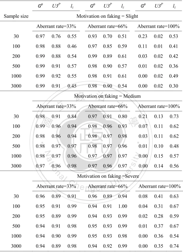
(3) Abstract. Faking detection is a crucial issue because of the effect on the hypothesized relation among variables, model testing, and test fairness. Aside from the Social Desirable Scale, which has often been used in detecting faking, we explored the possibility of an alternative method, which is the person-fit statistics of nonparametric item response theory (NIRT). In the scope of parametric item response theory (PIRT), the person-fit technique has been used in faking detection. Although the PIRT assumptions such as large sample size, normal distribution, and number of items are. 治政 difficult to achieve, numerous researchers still adopt conventional methods, leading to 大立 inaccurate results and implications. Using NIRT person-fit may be more flexible and ‧ 國. 學. closer to the practical condition based on NIRT features, and are therefore the focus. ‧. of this study.. sit. y. Nat. We used both simulated and real data to test the hypothesis. In Study 1, the data. io. er. were simulated and varied in sample size, distribution, faking motivation, and aberrant rate, to investigate the accuracy of person-fit estimating between PIRT and. al. n. iv n C NIRT. In Study 2, the techniquehusing person-fit U e n g c h i as a faking detection tool was applied to empirical data to evaluate its use in a practical context.. The results indicate that superior person-fit statistics are conditional. The Guttman error detection rate was higher when the sample size was less than 100, when partial item-faking existed in the scale, and in normal and platykurtic distributions. When the aberrant rate is 100% with severe faking, U3p outperformed other indicators in the negatively skewed and platykurtic distribution. Comparatively, lz could be adopted in all median-faking conditions. Our empirical study found that the normal distribution of ability is not easy to satisfy across a small and large sample. . i .

(4) size. Adopting person-fit statistics for faking detection is feasible, particularly for U3p.. Keywords: Nonparametric item response theory, faking, sample size, person-fit, R .. 立. 政治大. ‧. ‧ 國. 學. n. er. io. sit. y. Nat. al. . Ch. engchi. ii . i Un. v.

(5) 摘要在心理測驗中，作假的偵測是一個很重要的議題，因為其效果乃影響著變項間的關係、模型測試的正確性、以及測驗的公平性。目前，社會期許量表已被廣泛的應用於作假偵測，但增加題數，則亦增加作答者的負荷。因此，本研究欲探究應用 person-fit 統計數作為解決方法的可能性。雖然過去已有研究使用參數型的試題反應理論下的 person-fit 技術進行作假偵測，然而，參數型的試題反應理論的諸多假設，如：大樣本、常態分配、以及多題數等，在實際資料分析中並不容易滿足，因而導致不正確的結果及應用。據此，本研究乃聚焦於探究非參數試. 政治大. 題反應理論下的 person-fit 技術之應用效用，取其使用情境較彈性，且更接近實. 立. 際的情境之優點。. ‧ 國. 學. 本研究使用模擬資料及實際資料進行研究假設的檢驗。在研究一中，依據不同的樣本數、樣本能力分配、作假動機以及題目的異常率，以R產生模擬作答並. ‧. 求出 person-fit 數值，進而比較參數型與非參數型各 person-fit 指標的偵測率. sit. y. Nat. （detection rate），作為效用判斷之依據。研究二則將此技術應用於實際資料中，. n. al. er. io. 以社會期許量表與一份興趣量表進行本研究所採用之三種統計數（lz, U3p 與. v. Guttman errors）的偵測檢證，以瞭解其在實際情境中的實用性。. Ch. engchi. i Un. 研究結果指出，較佳的person-fit統計數需視不同的情境而定。Guttman errors 最適合用於當樣本數小於 100 人，受試者能力值為常態分配及低闊峰，而作答異常率僅為部分的情況。當作答異常率達到 100％，受試者能力分配為負偏態及低闊峰，且作假程度嚴重時，以U3p的偵測效果較佳。而lz則最適用於各種中等程度的作假情境。從實際資料的分析結果，指出不論是大樣本或小樣本，能力分配為常態性的假設皆不容易被滿足，且應用person-fit統計數於作假偵測是可行的，特別是使用非參數型的U3p指標。. 關鍵字：非參數試題反應理論、作假、樣本數、person-fit、R. . iii .

(6) Table of Contents Chapter 1 Introduction ...................................................................................................1 1.1 Background ......................................................................................................1 1.2 Statement of the Problem.................................................................................6 1.3 Limitations of the Study...................................................................................7 1.4 Glossary ...........................................................................................................7 1.4.1 Parametric item response theory...........................................................7 1.4.2 Nonparametric item response theory ....................................................8 1.4.3 Person-fit...............................................................................................8 Chapter 2 Literature Review..........................................................................................9 2.1 Person-fit..........................................................................................................9 2.1.1 lz...........................................................................................................14 2.1.2 Guttman errors ....................................................................................16 2.1.3 U3p ......................................................................................................18. 政治大 2.2 Person-fit and faking......................................................................................20 立 2.3 Sample Size and Distribution.........................................................................25 ‧. ‧ 國. 學. 2.4 The comparisons of PIRT and NIRT .............................................................31 2.4.1 The limitations of PIRT ......................................................................31 2.4.2 NIRT ...................................................................................................32 2.5 Nonparametric Estimation .............................................................................35 2.5.1 The comparison between parametric and non-parametric methods ...35 2.5.2 The assumptions of NIRT models ......................................................36 Chapter 3 Method ........................................................................................................44 3.1 Study 1: Simulation study..............................................................................45 3.1.1 Simulation design and variables .........................................................46 3.1.2 Data Generation ..................................................................................51 3.2 Study Two: Empirical-data application .........................................................54 Chapter 4 Results .........................................................................................................56. n. er. io. sit. y. Nat. al. Ch. engchi. i Un. v. 4.1 Simulation study ............................................................................................57 4.1.1 Detection rate of three indicators under different distributions and sample sizes. ................................................................................................57 4.1.2 Detection rate of three indices under different distributions and aberrant rates................................................................................................70 4.1.3 Detection rate of three indices under different distributions and faking degrees .........................................................................................................79 4.2 Study 2: Empirical study................................................................................88 4.2.1 Distribution under the given sample size............................................89 4.2.2 Social desirability scale and person-fit statistics ................................91 . iv .

(7) Chapter 5 Discussion and Conclusion .........................................................................95 5.1 Discussion on major findings.........................................................................95 5.1.1 Sample size .........................................................................................95 5.1.2 Faking degree......................................................................................97 5.1.3 Aberrant rate .......................................................................................98 5.1.4 The superior indicator .........................................................................99 5.1.5 The methods of data simulation........................................................100 5.2 Discussion on Empirical Study....................................................................101 5.3 Suggested steps for application....................................................................103 5.4 Limitations of Research ...............................................................................105 5.5 Suggestions for Future Research .................................................................107 References..................................................................................................................109 Appendix....................................................................................................................120. 立. 政治大. ‧. ‧ 國. 學. n. er. io. sit. y. Nat. al. . Ch. engchi. v . i Un. v.

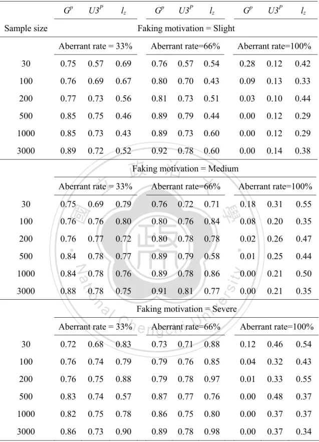
(8) List of Tables Table 1. Person-fit statistics.........................................................................................13 Table 2 Detection rate and false-positive rate of Gp and U3p for each type Ⅰ error 50 Table 3. The detection rate of three person-fit indices under Normal Distribution.....59 Table 4 Detection rate of three person-fit indices under a negatively-skewed distribution .....................................................................................................62 Table 5 Detection rate of three person-fit indices under platykurtic distribution........65 Table 6 Detection rate of three person-fit indices under a positively-skewed distribution .....................................................................................................68 Table 7 Factor loading and reliability coefficient........................................................89 Table 8 Descriptive statistics and normal distribution test by sample size .................91 Table 9 Detection rate of Gp, U3p, and lz by sample size ............................................93 . 立. 政治大. ‧. ‧ 國. 學. n. er. io. sit. y. Nat. al. . Ch. engchi. vi . i Un. v.

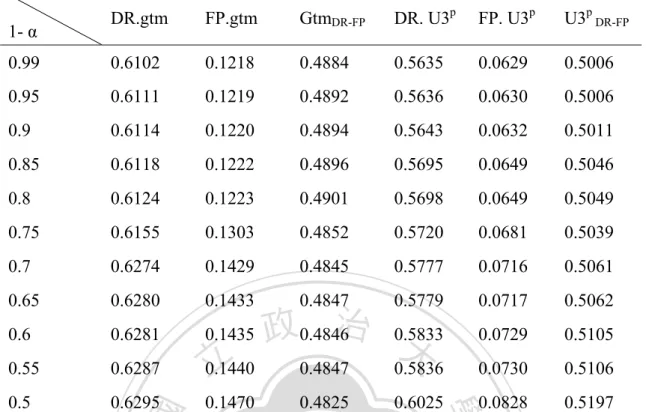
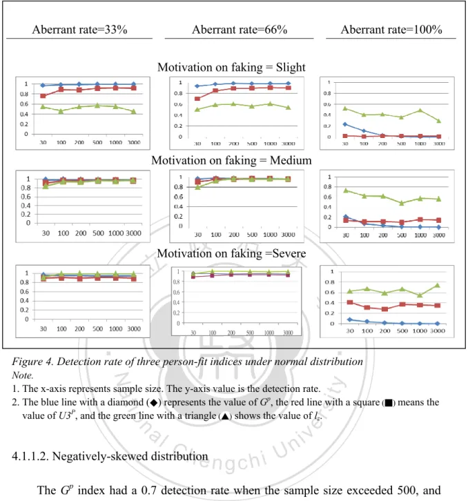
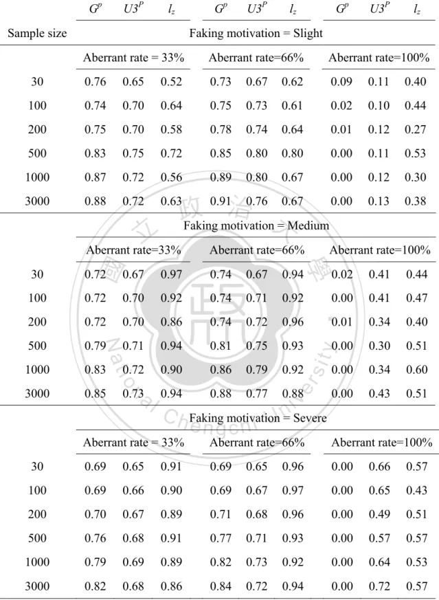
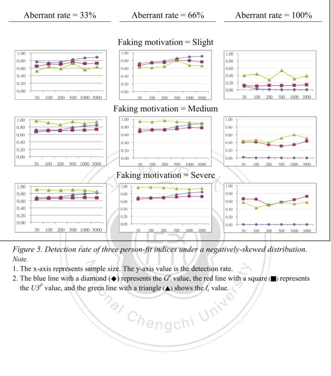
(9) List of Figures Figure 1. The IRFs of MHM (Left) and DMM (right) ................................................42 Figure 2. The relation among the models of PIRT and NIRT .....................................43 Figure 3. The value of gtmDR-FP and U3pDR-FP. .............................................................50 Figure 4. Detection rate of three person-fit indices under normal distribution ...........60 Figure 5. Detection rate of three person-fit indices under a negatively-skewed distribution. ..................................................................................................63 Figure 6. Detection rate of three person-fit indices under platykurtic distribution. ....66 Figure 7. Detection rate of three person-fit indices under platykurtic distribution. ....69 Figure 8. Detection rate of three indicators under different aberrant rates in normal distribution. ..................................................................................................71 Figure 9. Detection rate of three indicators under different aberrant rates in negatively-skewed distribution. ...................................................................73. 政治大 Figure 10. Detection rate of three indicators under different aberrant rates in 立 platykurtic distribution.................................................................................75 ‧. ‧ 國. 學. Figure 11. Detection rate of three indicators under different aberrant rates in positively-skewed distribution .....................................................................77 Figure 12. Detection rate of three indicators under different degrees of faking in normal distribution.......................................................................................80 Figure 13. Detection rate of three indicators under different degrees of faking in negatively-skewed distribution ....................................................................82 Figure 14. Detection rate of three indicators under different degrees of faking in platykurtic distribution.................................................................................84 Figure 15. Detection rate of three indicators under different degrees of faking in platykurtic distribution.................................................................................86 Figure 16. Eetection rate of three person-fit statistics by sample size.........................93. n. er. io. sit. y. Nat. al. . Ch. engchi. vii . i Un. v.

(10) Chapter 1 Introduction. 1.1 Background Tests are widely used, and are usually categorized into achievement tests and psychological tests. The former could be used to understand the condition of learning, and may be used as a determinant for school entrance (Yu, 2002). The latter could. 政治大. assist in identifying the personality and characteristics of individuals, and therefore,. 立. be used in the selection of employees (Chen, Lee, & Yen, 2004; Lai, Yu, & Hsu,. ‧ 國. 學. 2009). The purposes of using tests are to order and filter the participants. That is, the. ‧. results of the test have a benefit-based relationship to participants, such as pass or fail,. Nat. io. sit. y. and accept or reject. Therefore, participants are likely to provide answers that will. er. benefit them. These types of answers lead to an unmatched test score and the real. al. n. iv n C ability of the participant, and also h create e nunfairness g c h i inUthe test. As such, to obtain the true ability or latent feature score of the participant would be a vital task for test expert. That is, we have to accurately and immediately detect faking, which could maintain the fairness of the test. There are two main methods used to detect faking behavior in psychological tests in common. The first method is by means of the Social Desirability Scale. If participants have a higher score in the scale than a pre-determined cut-off score, then. . 1.

(11) the faking behavior is confirmed. The second method is by using force choice questions. This method avoids faking by arranging the types of test items (Chen et al., 2004). These methods are used to determine whether the answers represent the true ability or latent trait of participants. The concept of person-fit provides a similar function. Person-fit concerns the atypical test performance (Emons, 2008; Meiler & Sijtsma, 2001), and is based on the level of dependency between item-score patterns. 政治大. and individual response patterns (LaHuis & Copeland, 2009; Meijer & Sijtsma, 2001).. 立. Therefore, person-fit is an alternative method to detect faking.. ‧ 國. 學. A number of studies consider the level of person-fit as an indicator of faking.. ‧. Schmitt, Chan, Sacco, McFarland and Jennings (1999) used lz under parametric item. Nat. io. sit. y. response theory as an indicator of faking in personality tests. LaHuis and Copeland. er. (2009) used the person-fit technique in a multilevel logistic regression approach to. al. n. iv n C h eindicated explore faking. Schmitt et al. (1999) the slope variance of a person’s n g c hthati U response curve (PRC) reflected the phenomenon in which participants try to score a higher value, which leads to an inferior person-fit. Zickar and Drasgow (1996). claimed that the method of parametric item response theory to examine faking was more effective than using the Social Desirability Scale, to categorize faking and non faking participants. It can be known that using person fit as an alternative technique of detecting faking was not new. But if the efficiency can maintain cross various. . 2.

(12) conditions, such as non-normal distribution and small sample, is a pending issue which would be investigated in the current study. Person-fit is a type of technique in the scope of item response theory. The parametric item response theory (PIRT) has been widely used; however, the nonparametric item response theory (NIRT) is becoming a preferred choice (Cliff & Keats, 2003; Sijtsma & Molenaar, 2002; Stout, 1990). Mokken (1971) proposed the. 政治大. theory, and a set of procedures for dichotomous items, which is known as Mokken’s. 立. scale analysis. The development followed the methods of estimation, software. ‧ 國. 學. application, and the various types of models. The models of NIRT have been. ‧. developed from dichotomous to polytomous items. Applied Psychological. Nat. io. sit. y. Measurement (2001) devoted a special issue to discuss the NIRT. These provide. er. strong evidence to the drastic development of NIRT. The NIRT could be applied to. al. n. iv n C h e nandg cSijtsma similar areas or topics as PIRT. Junker h i U(2001) applied the technique to. cognitive analysis and claimed the applicability under the fewer limitations of NIRT. Sijtsma, Emons, Bouwmeester, Nyklicek and Roorda (2008), and Stewart, Watson, Clark, Ebmeier, and Deary (2010), found that the model of NIRT could efficiently match the data format in scale analysis. In differential item function (DIF), Glickman, Seal and Susan (2009) conducted the study by using nonparametric Baysian estimation to diagnose the DIF in the IRT model. Emons (2008) conducted a. . 3.

(13) simulation study to investigate the stability of person-fit detection under the scope of NIRT, and asserted the effectiveness of unusual pattern detecting. Nozawa (2008) and Xu (2004) applied the model of NIRT to the study of computer adaptive test, and compared the adaptability between PIRT and NIRT in nonequivalent group design. As such, the development and widespread applications of NIRT are apparent. It has been from cognitive measurement to psychological test, from dichotomous to. 政治大. polytomous. The NIRT is highly efficient in a number of common fields, such as DIF,. 立. computer adaptive testing, and person-fit.. ‧ 國. 學. The use of NIRT offers a number of advantages. The nonparametric item. ‧. response theory was created because the premises of the parametric item response. Nat. io. sit. y. theory do not fit in a number of conditions. Those premises, which include the. er. distribution type of population ability, ordinal scale, but not continuous scale, and the. al. n. iv n C h e n g c hagreed requirement of sample size, are conventionally i U upon. The fewer limitations and unreal assumptions in the usage of NIRT, in comparison to PIRT, may result in a better fit and more real conditions (Meijer & Baneke, 2004). Chernyshenko, Stark, Chan, Drasgow, and Williams (2001) state that, compared to the two-parameter graded response model and the three-parameter graded response model (abbreviated as 2 PL and 3PL, respectively, with PL meaning that the model is estimated by logistic function)(Osterlind & Everson, 2008), the nonparametric item response model. . 4.

(14) may achieve a better fit in analyzing a Sixteen Factor Personality Scale. Due to the calculation of the simple covariance structure between items and nonparametric regression in the NIRT model, it is easier to interpret and understand the results, also to use the software. The required sample size is relatively small in NIRT for conducting a confidential measurement of psychological properties (Emons, 2008). The sample size is an issue especially for mixed-method, which is currently the. 政治大. common method, one hundred participants recruited for interviews or observations. 立. are a really exhausted work; however, this sample size is still small for quantitative. ‧ 國. 學. analysis. The sample size affects the choice of analysis under the premise of a number. ‧. of statistic methods, and may limit the contribution of the research. Based on the. Nat. io. sit. y. sections above, measuring the person-fit under the NIRT model is a superior. er. developmental method. Meijer and Sijtsma (2001) conducted a comprehensive review. al. n. iv n C U of merits and demerits of of the measurement of person-fit, h andeidentified n g c hai number. classical test theory and item response theory in person-fit measuring. They also stated that further research is required on the model-free and robust methods of NIRT model. The roles of PIRT and NIRT in relation to each other are compensatory rather than opposite. Point estimation may be provided by PIRT, therefore it is more applicable and widely used when conducting estimation and calculation (Yu, 2009).. . 5.

(15) PIRT is more applicable than NIRT when real data meets the premises of PIRT (Nozawa, 2008). However, the assumptions and premises, such as normal distribution of data, interval scale, and sufficient sample size are not easy to achieve (Dyehouse, 2009). As such, it is essential to develop a method which is easier and closer to the real situation. Various studies have investigated the relation between person-fit and faking detection under the definition of PIRT (Zicker & Drasgow, 1996), and the. 政治大. exploration of analytic techniques for polytomous items of NIRT (Emons, 2008).. 立. However, there is limited research on the effectiveness of using person-fit to detect. ‧ 國. 學. faking in NIRT.. ‧. Therefore, the study intends to investigate the detection rate between NIRT and. Nat. io. sit. y. PIRT on person fit statistics under several potential empirical issues, such as sample. n. al. er. size and distribution of ability, to provide appropriate evidence for the usage under the less constraint model.. Ch. engchi. i Un. v. 1.2 Statement of the Problem According to the purpose of the study, the present study aims to investigate three main questions. The purposes of this study are (1) to explore the possibility of using person-fit as a technique to detect faking when the sample size, distribution of ability, aberrant rate are varied, and (2) compare the efficiency between the person fit. . 6.

(16) statistics of PIRT and NIRT (study one). Finally, (3) to verify the results from simulation study in the context of real data (study two).. 1.3 Limitations of the Study This study is conducted by using simulated data and real data to achieve theoretical and practical understanding. In the simulated portion, the variables. 政治大. included the numbers of sample size, the distribution of ability, and the aberrant rate.. 立. With regard to other variables, such as the methods of estimation, although they may. ‧ 國. 學. have an impact on the estimation of person-fit, they are not the main consider issues. n. al. er. io. sit. y. Nat. 1.4 Glossary. ‧. in this study. These variables will be set as a fixed value.. 1.4.1 Parametric item response theory. Ch. engchi. i Un. v. Parametric item response theory is one of the models of item response theory; and defined the relation between item score and latent ability (trait) by parametric functions, such as logistic or ogive function (Sijtsma, 2005). The parameters generally included difficulty, discrimination, and guess. The item characteristics curve, derived from the three parameters, is used to describe the relation between latent ability and the probability of a correct answer (Yu, 2009).. . 7.

(17) 1.4.2 Nonparametric item response theory Nonparametric item response theory is one of the models of item response theory; and is adaptive when the item scale is ordinal. The only assumption of this model is that the relation between score and ability is order. The discrepancy between NIRT and PIRT is that each item function may not have to follow the discipline of logistic monotonous function (Sijtsma, 2005).. 政治大 Person-fit refers to the issues of the unusual response pattern (Meijer, &Sijtsma, 立. 1.4.3 Person-fit. ‧ 國. 學. 2001). Person-fit could be indicated by the level of discrepancy between the assumed. ‧. IRT models or item-score pattern and the individual response pattern (LaHuis &. sit. y. Nat. Copeland, 2009; Meijer & Sijtsma, 2001). The person-fit statistics are used to detect if. n. al. er. io. the examinee had unusual item response patterns, and to distinguish them from. Ch. normal respondents (Katabatsos, 2003).. . engchi. 8. i Un. v.

(18) Chapter 2 Literature Review. Five sections are used to explain the relative theories and previous studies. The first section introduces the concept and indicators of person-fit. Follows are some reviews on the studies about faking detection via person-fit. The third section offers an explanation of the role of sample size, the need for sample size in this study, and. 政治大. the advantages of NIRT in the sample size. The comparison between PIRT and NIRT. 立. estimates, and demonstrate the theory and model of NIRT.. ‧ sit. y. Nat. 2.1 Person-fit. 學. ‧ 國. follows the third section. Lastly, the study illustrates the methods of non-parametric. n. al. er. io. Person-fit refers to the level of consistency between the assumed IRT models or. Ch. i Un. v. item-score pattern and the individual response pattern (LaHuis & Copeland, 2009;. engchi. Meijer & Sijtsma, 2001). This issue concerns atypical response patterns (Meijer, & Sijtsma, 2001), and the methodology of person-fit could test invalid responses (Emons, 2008). Parametric and non-parametric estimates can analyze the person-fit. Parametric estimate is the measurement of the difference between test scores and the predicted values in the assumed model. Conversely, the person-fit value of non-parametric. . 9.

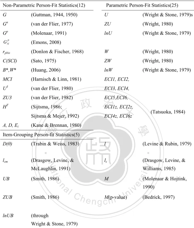
(19) estimate is not based on the test response model parameters, but rather calculates the responses of all testers (Karabatsos, 2003). Both methods, in dichotomous items, are commonly discussed (Karabatsos, 2003; Meijer & Sijtsma, 2001;van Krimpen-Stoop & Meijer, 2002).. However, there is limited research which analyzes both methods in. polytomous items (Glas & Dagohoy, 2007), especially for non-parametric estimate. The topics of most studies focused on parametric estimates in cognitive tests. 政治大. (Dagohoy, 2005; van Krimpen-Stoop & Meijer, 2002) and non-cognitive tests (Reise,. 立. & Widaman, 1999; Zickar, Gibby, & Robie, 2004).. ‧ 國. 學. There has been several statistics proposed to represent the statistics of person-fit.. ‧. Karabatsos (2003), the most completed one in our knowledge, integrated 36 indicators.. Nat. io. sit. y. Those statistics are divided into two parts, parametric and nonparametric methods,. er. and are shown in table 1. There are more than one index for investigating person fit. al. n. iv n C h e n gtheory though, the indices are based on different c h i andU might have merits for certain condition. St-Onge, et al(2011) asserted that the lz is IRT-based indices, which are used in studies due to the relatively high detection rate, while U3p is belonged to the group-based person fit statistics, which is superior in correctness and wide usage. With regard to the potency between nonparametric and parametric method, some comparative study have been conducted. In St-Onge, et al.(2011) study, consider the range of item difficulty, discrimination, test length, and two parametric person fit. . 10.

(20) indicator, l z and ECI2z, and two nonparametric person fit indicators, HT and U3, were compared on the detection rate for aberrant response pattern. They found the nonparametric indices, HT and U3 , have higher detection rate than the two parametric methods for a fixed aberrant rate of 0.6 under the simulated condition of cheating. Also, a number of studies indicate that the U3 and Guttman error may have lower detecting rates; however, Emons (2008) provided evidence that the detecting rates are. 政治大. similar to the Guttman error and l z by a simulation study. That means that the. 立. nonparametric method could have a similar power to PIRT, and could perform. ‧ 國. 學. superior than parametric indices.. ‧. In the scope of nonparametric indices, the Guttman error is the effective method. Nat. io. sit. y. to detect misfit, while it is easily affected by total score, especially for examinees with. er. higher and lower scores. Karabatsos (2003) stated that for dichotomous items, HT, C,. al. n. iv n C MCI, and U3 performed optimally h in e ann aberrant i U It should be noticed that the g c hpattern. four statistics are nonparametric methods. Furthermore, by comparing 36 statistics of person-fit in detecting rate, Karabatsos (2003) stated that U3 is the one of the strongest indicators in the top four. Accordingly, all indices have certain condition to favor. Based on the purpose of comparisons in this study, the proper indices in both nonparametric and parametric method would be selected to investigate the efficiency under the factors of this study.. . 11.

(21) lz is one of the commonly used indicators, and Guttman and U3p are the more stronger of nonparametric person fit indices, based on previous studies. Three types of indicators, lz, Guttman errors, and U3p, are introduced in this study, which are related to this study. The other indicators could refer to those in the study of Karabatsos (2003). The three types of indicators are as follows.. 立. 政治大. ‧. ‧ 國. 學. n. er. io. sit. y. Nat. al. . Ch. engchi. 12. i Un. v.

(22) Table 1. Person-fit statistics Non-Parametric Person-Fit Statistics(12). Parametric Person-Fit Statistics(25). G. (Guttman, 1944, 1950). U. (Wright & Stone, 1979)s. Gn. (van der Flier, 1977). ZU. (Wright, 1980). Gp. (Molenaar, 1991). lnU. (Wright & Stone, 1979). G. P N. (Emons, 2008). rpbis. (Donlon & Fischer, 1968). W. (Wright, 1980). C(SCI). (Sato, 1975). ZW. (Wright, 1980). B*,W*. (Huang, 2006). lnW. (Wright & Stone, 1979). MCI. (Harnisch & Linn, 1981). ECI1, ECI2,. 3. U. (van der Flier, 1980). ECI3, ECI4,. ZU3. (van der Flier, 1982). ECI5,ECI6,. (Kane & Brennan, 1980). 學. A, D, Ei. Item-Grouping Person-fit Statistics(5) l. lzm. (Drasgow, Levine, &. lz. (Levine & Rubin, 1979). ‧. (Trabin & Weiss, 1983). (Drasgow, Levine, &. y. Nat. D(θ). Williams, 1985). io. (Smith, 1986). (Smith, 1986). lnUB. (through. (Molenaar & Hojtink,. M. al. v ni. n. ZUB. sit. McLaughlin, 1991) UB. (Tatsuoka, 1984). Ch. er. H. 政治 (Sijtsma, 1986; ECI1z, ECI2z, 大 Sijtsma & Mejer, 1992) ECI4z, ECI6z 立. ‧ 國. T. e n g cM(p-value) hi U. 1990). (Bedrick, 1997). Wright & Stone, 1979). Resource: Karabatsos, G. (2003). Comparing the aberrant response detection performance of thirty-six person-fit statistics. Applied Measurement in Education, 16, 277-298. Huang, T. W. (2006). Aberrant response diagnoses by the Beyond-Ability-Surprise index (B*) and the Within-Ability Concern index (W*). Proceedings of 2006 Hawaii International Conference on Education, Honolulu, Hawaii, pp. 2853-2865. Emons, W. H. M., Meijer, R. R., & Sijtsma, K. (2002). Comparing simulated and theoretical sampling distributions of the U3 person-fit statistic. Applied Psychological Measurement, 26(1), 88-108.. . 13.

(23) 2.1.1 lz This is one of the commonly used indicators; and represents the compound probability of responses and estimated ability. Mostly, according to the concept of person fit, the indices could be expressed as formula 1（Snijders, 2001）.. k. ∑ X w (θ ) − w (θ ) i =1. i. i. (1). o. 政治大. Where wi (θ ) and wο (θ ) are the suitable function.. 立. If we let a person-fit statistic with expectation 0, the person fit statistics are. ‧ 國. 學. expressed in the form of formula 2, which is a centered form.. ‧ y. Nat. k. io. n. al. (2). er. i =1. sit. V = ∑ [ X i − Pi (θ )] − wi (θ ). Ch. engchi. i Un. v. Most studies conducted the indices by log likelihood function, shown as formula 3. The form of log-likelihood function of V, let be abbreviated as l, verifies person-fit via the likelihood of item parameters (ex: under one, two or three parameters) and the estimated theta (St-Onge et al., 2011). The index was proposed by Levine and Rubin(1979) originally. Then was further developed by Drasgow, Levin and Williams(1985) and Drasgow, Levin and McLaughlin(1991).. . 14.

(24) [. ]. l (θ i ) = ∑ {X ij ln Pj (θ i ) + (1 − X ij ) ln 1 − Pij (θ i ) } n. (3). j =1. Formula 3 is the calculation of l, where Xi is the score on item i in a scale with n items. However, the calculation of l would cause two major problems: 1. Since l is not the standardized score, researchers have to relay on θ to classify individual into normal or aberrant. That is, the statistics is not independent enough; 2. Researchers. 政治大. need a null assumption distribution of fitting response behavior to classify an item. 立. response pattern as aberrant. According to the problems above, which are theta. ‧ 國. 學. dependent and an unknown sampling distribution, Drasgow et al.(1985) pointed out. standard. normally. distributed. y. asymptotically. (Meijer. &. van. io. sit. a. Nat. assumed. ‧. the method of standardizing l . The method could reduce the interference of theta, and. er. Krimpen-Stoop, 2000). That is, the value of standardizing l, lz, would not be. al. n. iv n C is n as formula influenced by θ. The calculation ofhlz e g c h i 4,Uwhere E(l) is the expected value of l，Var(l) refers to the variance of l. The negative lz indicates insufficient fit. The response patterns are different from the predicted value compound by item difficulty and individual ability. The large number and negative values indicates an inferior fit (Armstrong, Stoumbos, Kung, & Shi, 2007; Meijer, 2003). Since the conditional null distribution of lz is standard normal as the test length is long enough, the critical value set as -2 generally (Ferrando & Lorenzo, 2000).. . 15.

(25) lz =. l − E (l ) Var (l ). (4). k. E (l ) = ∑ {Pi (θ ) ln[Pi (θ )] + [1 − Pi (θ )]ln[1 − Pi (θ )]}. (5). i =1. ⎡ P (θ ) ⎤ Var (l ) = ∑ Pi (θ )[1 − Pi (θ )]⎢ln i ⎥ i =1 ⎣ 1 − Pi (θ ) ⎦ k. 2.1.2 Guttman errors Molenaar (1991),. 2. (6). 政治大 underlying the NIRT, suggested 立. using the value of the. ‧ 國. 學. Guttman error as the indicator of person-fit. The value is derived by calculating the. ‧. number of difficult items (or item-steps) that were passed and the number of easy. sit. y. Nat. items (or item-steps) that were failed. A large value indicates an inferior person-fit. n. al. er. io. (Emons, 2008). The indicator could be apply on dichotomous (denoted as G) and. Ch. i Un. v. polytomous cases (denoted as Gp). In dichotomous scale, for example, there are five. engchi. items ordered from easy to difficult as A, B, C, D, and E. The response pattern of examinee J is 10101, where 1 is correct, otherwise, 0. The Guttman errors are then three (the violated pattern is BC, BE and DE). For examinee K, the response is 00111, then the G is six (the violated pattern is AC, AD, AE, BC, BD, and BE). As for the polytomous scale, the calculation of the Guttman errors are based on the all possible item-step pairs, which the easy step failed and the difficult item step. . 16.

(26) passed. For example, there are two items with three item steps for each. We denote ∧. the item step difficulties as π jx j ，and let the π. jx j. as the sample estimate. It represents. the probability of score χj in the item J. The three item-step difficulties of item 1 are π11=.90, π12=.50, π13=.20. Similarly, the three step difficulties of item2 are set as π21=.80, π12=.70, π13=.30. It is known that the easiest step of those six is the step 1 of item 1. The passing rate goes to 90%. The next one is the step 1 of item 2. The. 政治大. passing rate is 80%. The step2 of item 2 is the third easiness. The passing rate is 70%.. 立. The most difficulty is the step 3 of item 1. The through rate is just 20%. If there is a. ‧ 國. 學. respondent score 3 in item1 and 1 in item 2. That means the respondent pass the step 3. ‧. of item1 but fail the step 2 and 3 of item 1 which are more easier. In this case, all of. Nat. io. sit. y. the item-step pair which failed in easier step and passed in difficult one would be. er. calculated. The number is the Guttman errors for polytomous scale (Emons, 2008).. al. n. iv n C We can model the Guttman h errors e n asg cformula h i U(7) for both dichotomous and. polytomous test. Let y represents the item-step score variable, and we can score 1 if the item-step is passed, otherwise 0. When the M in (7) equal to 1, the statistic represents the Guttman errors of dichotomous items (Meijer & Sijtsma, 2001), however, the flaw of the Guttman error is that it is dependent on total score.. JM. G = ∑ yk(1-yi). (7). l <k. . 17.

(27) For the comparison of each value of G, the statistics was normed by the item-step difficulties and the maximum possible given total scores. The form of normed Guttman error is denoted by Gp and the model is as the formula(8), where the X+ represents the sum of score.. G. P. =. G. max(G. (8). X +). 政治大. The software of Mokken’s scaling program (MSP) and mooken package in R can. 立. ‧ 國. 學. calculate the Guttman errors for each subject, which can be saved in another file for researchers to use (van Schuur, 2003, van der Ark, personal communication,. ‧. November, 2011).. er. io. sit. y. Nat. 2.1.3 U3p. al. n. iv n C h e n gerrors, Considering the flaw of the Guttman c h ivanUder Flier (1980) developed the. U3 as an alternative person-fit statistic, which is under the nonparametric statistics (Meijer, Molenaar, & Sijtsma, 1994). In concept, it is based on a log ratio of response vectors with the group’s correct response proportion for each examinee (St-Onge et al., 2011). U3 considers the value and order of item difficulty. Given a dichotomous scale with J items, χ j (j=1,…,J）, 1 represents the correct answer, and 0 means wrong answer. There would be a random vector comprised by the response pattern, denoted. . 18.

(28) as X. Also, we use the symbol of X+ to represent unweighted total score, which X + = ∑J X j . Accordingly, the value of U3 could be obtained by the formula (9). j =1 Given πj (j=1,…,J) is the proportion of the correct response on item j of the population, and its estimate by sample is denoted as π . The π is assumed to be in the order of ∧. ∧. j. π. ∧ 1. ≥. π. ∧. ∧ 2. ≥… ≥π J. j. . Under the fixed X+, all terms in the formula (9) are constant except. the w(x).The value ranges from 0 to1, where 0 represents the response pattern as an. 政治大. ideal Guttman pattern, that is, if and only if the respondent’s item score pattern is a. 立. 學. further from perfect Guttman patterns.. j =1. j. )−. j. j = J − x+ +1. ∧. πj. J. W (X ) = ∑ j =1. Xj. a∑l log(1 −π ) iv n Ch π engchi U J. n. π ∑ log(1 − π X+. j. er. j. y. ‧. π. J. log( ) − ∑ X j log( ) ∑ 1−π j 1−π j j =1 j =1. io. U3(X)=. π. Nat. X+. sit. ‧ 國. Guttman pattern(Emons, 2002). The larger value indicates that the pattern deviated. j. (9). j. (10). log( ) ∧ 1− π j. U3 can be used in polytomous items as well. The value was defined as formula (11), which is added the numbers of response category, M. The value, denoted as U3p, represents the sum of log odds of the item-step difficulties of the steps that were passed. The normed W(X) is used to obtain the generalization value of U3p, denoted. . 19.

(29) by U3p is shown as formula (12). The range of U3p is from 0 to 1. The value of 0 means no misfit, and 1 indicates extreme misfit. The max(W|X+) in formula(12) would occur when the easiest item steps of X+ are passed. The formula (13) is the expression of the condition of max(W|X+)(Emons, 2008).. ∧. πj. JM. W (X ) = ∑ j =1. U3 = p. Xj. (11). log( ) ∧ 1−π j. max(W X + ) − W ( X ). 立. max(W X + ) − min(W X + ) X+. 政治大. ∧. ‧ 國. 學. max(W X + ) = ∑ log it (π j ). (12). j =1. (13). ‧ sit. y. Nat. Where M means the numbers of response category. J represents the numbers of. n. al. er. io. items. X+ means the total score.. Ch. engchi. i Un. v. 2.2 Person-fit and faking The phenomenon of response set would appear in the personality test. Response set means that subjects tend to respond in a particular manner, such as center-tendency, guess, and affected by social desirability (Guo, 1985). Among these causes of response set, the tendency of social desirability is most considered by test. . 20.

(30) experts (Chen et al., 2004). Generally, the faking is defined as the response tends to social desirability (Lai, 2010). Two common methods are used to examine faking. The first one is by using forced choice questions in the items arrangement. This method sets the levels of social desirability in each alternative to be equal; therefore, examinees could not be affected by social desirability. The second method is by using the social desirability scale,. 政治大. which examines social desirability. The description of items consists of two parts,. 立. including the good behaviors, defined by the culture, which most people cannot. ‧ 國. 學. achieve, and the bad behaviors, which most people would act out (Marlowe &. ‧. Crowne, 1960). If the total score in this scale is more than a given value, the examinee. Nat. io. sit. y. would be judged as faking, which implies that the other items of the tests would also. er. be faked (Lai, 2010). However, the forced choice questions are difficult to arrange. If. al. n. iv n C h e n gthe the examinee displays both characteristics, i Uchoice might lead to an untrue c honly answer instead. Comparatively, the social desirability scale is easier and more convenient to use and implement (Chen et al., 2004). Nevertheless, the desired goal of each method is to detect atypical response patterns and to eliminate them. The concept of traditional methods to detect faking is similar to the construct of person-fit. The statistics of person-fit reflects the phenomenon that the response varied as the model predicted, when the difficulty of items increases, such as whether. . 21.

(31) the probability of adornment reduces when the difficulty varied (LaHius & Copeland, 2009). The difference between the value predicted by the model and the data may reflect the lack of motivation or faking in the test. The discrepancy would impact the validity of the interpretation of the test and results (Emons, 2008). Compared to the traditional method, one of the advantages of using person-fit as the means to detect faking is that we could explore how faking affects the measurement properties of. 政治大. items and scale. Distinct from prior studies focused on the implications of faking,. 立. such as, the exploration of the difference of faking between employee and applicants. ‧ 國. 學. (Lai, 2010), and to determine the proportion of faking that is reduced when. ‧. participants were posted in the context of “easy to fake” and “not easy to fake”. Nat. io. sit. y. (LaHuis & Copeland, 2009); This study focuses on the property of measurement.. er. A number of possible reasons for the aberrant pattern have been discussed. The. al. n. iv n C reasons included cheating, creativehresponse, e n g cguessing, h i Ucareless, and random response (Meijer et al., 1994; Karabatsos, 2003), as well as carelessness and inattention,. tendency to choose extreme response options, and reversed scoring (Emons, 2008). Reise (2000) stated that two perspectives are used to investigate the person misfit. The first perspective considers misfit as systematically deviate from the normal response. Under this point of view, it is originated from measurement error, such as answer in the wrong item or misunderstood the item description. The carelessness and. . 22.

(32) inattention were belonged to this category. The second perspective is the systematic difference among groups. That is, different level misfit resulted from level faking. In this viewpoint, researchers have to correct the effect of faking to obtain true ability. LaHuis and Copeland (2009) extended the second perspective to propose that the discrepancy between true ability and scores reflects the faking, and can be predicted by other variables, such as honesty and job desirability. In a particular context, the. 政治大. systemic bias in the response curve would correspond to the spurious response, due to. 立. the individual trying to achieve a higher score on certain items.. ‧ 國. 學. The causes of atypical responses could be discussed from achievement test and. ‧. psychological test separately. In psychological tests, faking might have two possible. Nat. io. sit. y. reasons. One is that it occurred unconsciously since the false personality has been. er. adopted by the individual; the other one is that respondent fakes purposely. The. al. n. iv n C h easnthe faking in psychological test is defined one, and which is also the target hi U g csecond. of social desirability scale (Lai, 2010). The motivation to fake might be shown in several ways, such as choose extreme response options, and reversed scoring. Those are distinct from the reasons in achievement test, in which, the atypical response could be explained by cheating, creative response, guessing. As for the random response, some technique of detecting invalid survey could be adopted. Therefore, it could be assumed and tested that the atypical response is aroused mainly by faking. . 23.

(33) motivation in psychological (personality) test, there might have other miner factors though. Person-fit, as an indicator of faking, has been discussed in prior studies (Schmitt et al., 1999; Zicker & Drasgow, 1996). LaHuis and Copeland (2009) used multilevel logistic regression to generate the value of person-fit, and to investigate the relationship between faking and simulated dichotomous and polytomous data. They. 政治大. found that person-fit is an effective predictor to the motivation to fake. However, their. 立. study was conducted under the parametric method with 1000 examinees, and 20 items.. ‧ 國. 學. Besides, the data was simulated from GRM, and did not have an adequate model fit.. ‧. Chernyshenko et al. (2001) suggested that the nonparametric model could achieve a. Nat. io. sit. y. better fit than GRM in a personality test. Emons (2008) investigated the relationship. er. between Gp and aberrant responses. The study was conducted under the. al. n. iv n C h e n gwere nonparametric model, and 1000 examinees i Uin the process. A small sample c hused was not the main point of the study, yet the advantage of the nonparametric model was not demonstrated in the study. Zicker and Drasgow (1996) compared the effectiveness of faking detection between person-fit and the social desirability scale, and indicated that it is more effective to use person-fit rather than the social desirability scale. A total of 48,725 participants were involved in that study, using the parametric person-fit.. . 24.

(34) Using person-fit as a predictor is feasible, theoretically and practically, in the above-mentioned study. Prior studies explored the relation, and conducted a comparison between person-fit and social desirability. However, these studies used the model of parametric method, and a large sample size. The advantages of NIRT, such as the small sample size and distribution free, have not been discussed. This study investigates whether the effectiveness of this method can be maintained in the. 政治大. small sample size and non-normal distribution.. 立. ‧ 國. 學. 2.3 Sample Size and Distribution. ‧. The sample size may influence the results or interpretation of the statistics;. sit. y. Nat. however, it is a low priority issue in research concerning funding or budgets. The. n. al. er. io. sample size is vital, as it relates to two important factors, which are the error of. Ch. i Un. v. sampling and power (Maxwell, Kelley, & Rausch, 2008). The error of sampling. engchi. represents the level of mis-specificity in the process of sampling. A large sample size may reduce the standard error of sampling, and the error of interpretation. Therefore, “more is better” could refer to the required sample. The power symbolizes the ability to reject an accurately false null hypothesis. It can be used as the evidence to calculate the reasonable sample size in a study. Generally, a large power requires a higher cost; however, a small power may limit the ability to discover the true ability (Chiou, 2008).. . 25.

(35) Researchers tend to obtain large sample sizes to improve the interpretation of the results, yet, it is crucial to determine how small the sample should be under an acceptable estimation. Another factor which affects the representativeness is the distribution of sample ability or the assumed distribution in the given technique. The common methods set a normal distribution as the default distribution, which means that the method can be. 政治大. used when the ability fits the premise. The estimation would be affected by the. 立. distribution of ability. For example, when using the method based on parametric item. ‧ 國. 學. response theory, the skewed distribution would lead to less accuracy estimation than. ‧. in a normal distribution (Seong, 1990; Stone, 1992; Swaminathan & Gifford, 1983;. Nat. io. sit. y. Yu, 2009). That is, we could only benefit from IRT when a large sample is used (Liu,. er. 2007), as the normal distribution is easier to be satisfied in the large sample.. al. n. iv n C U size h ethen required research, g c h i sample. In the PIRT related. was determined by. considering a number of factors, such as the numbers of parameter, the method of estimation, and test length. As such, the required sample size is varied by different models, and in different conditions. Wright and Stone (1979) state that the Rasch model require a minimum of 20 items and 200 examinees. For 2PL models, 30 items and 500 examinees are required. In 3PL models, 60 items with 1000 examinees, or 30 items with 2000 examinees are required (Hulin, Lissak, & Drasgow, 1982).. . 26.

(36) A number of studies have investigated the sample issues in PIRT. For 2PL models, de Ayala (2009) suggested that 500 participants with 20 items are required to obtain reasonable results of estimation. Drasgow (1989), when considering the method of estimation, by using marginal maximum likelihood estimation (abbreviated as MMLE), the acceptable standard error can be obtained by 200 examinees with 20 items, however, the α and δ cannot be extreme. Also using MMLE, Seong (1990). 政治大. used 45 items to explore the effect of distribution. The types of distribution are. 立. normal, positively skewed and negatively skewed. Sample sizes are 100 and 1000.. ‧ 國. 學. The results indicated that the estimations are more accurate when the assumed. ‧. distribution is consistent with the distribution of real data. The estimation of the. Nat. io. sit. y. parameters of difficulty and discrimination are stable when the sample size is 500. er. with 20 items, which were compared with different distributions (normal, positively. al. n. iv n C U 1000) and items length (10, h e nsize skewed, symmetry, playtkurtic), sample h i 500, g c(250,. 20, 40)(Stone, 1992). Harwell and Janosky (1991) investigated the relationship between accuracy and assumed theoretical distribution. Using BILOG, they found that a short item length (15 items) and small sample size (75, 100, and 150) would result in inaccurate estimation, while using 25 items and more than100 examinees could not be affected by prior distribution.. . 27.

(37) In 3PL models, using MMLE to estimate accurate parameters could be obtained by symmetric distribution of ability, and have 1000 examinees with 20 items (de Ayala, 2009). Mislevy (1986) also obtained similar results. Ronald (1997) also confirmed this but from another manner. A stable item parameters measurement could not be obtained in a small sample and short test under the 3PL model. Yen (1987) explored the relationship and influence among 1000 simulees and different types of. 政治大. distribution (normal, negatively skewed, positively skewed, and platykurtic), item. 立. length (10, 20 and 40 items) and computer programs for analysis (BILOG and. ‧ 國. 學. LOGIST) in a Monte Carol study. The procedure of LOGIST was used to produce. ‧. maximum likelihood estimates by Lord (1974), while BILOG also offers the option of. Nat. io. sit. y. Bayesian estimation procedures that are not available in LOGIST (Mislevy & Bock,. er. 1984). Using BILOG, the results showed that 20 items and 40 items are more accurate. al. n. iv n C than 10 items in the estimation of h discrimination i Udifficulty. If there are 10 items, e n g c hand then BILOG is more accurate than LOGIST. That is, for fixed short items, a different procedure of calibration could generate a different estimator. The accuracy of estimation is affected mainly by sample size, distribution of ability, tests of lengths, and the procedure of estimation. These factors may be compensating for each other to obtain reasonable results. For a 3PL model, a sample size of 1000 would be ideal (Yu, 2009).. . 28.

(38) Some studies have different view about the relationship between the sample and the usage of IRT. Reise & Yu(1990) investigated the parameter recovery of 2PL Graded Response Model, and analyzed by MULTILOG. The sample size, included 250, 500, 1000, and 2000, was one of the manipulated variables. The results indicated that the size of sample was not the main concern as for estimating theta. There was no different between 250 and 500 persons on recovery rate. That means, the efficiency of. 政治大. theta estimation are equal for 250 and 500 persons with 25 items with 5 categories.. 立. St-Onge et al. (2009) conducted a Monte Carlo study to investigate the possibility of. ‧ 國. 學. using nonparametric method in ICCs estimation for arising the accurate rate of. ‧. IRT-based person fit to under small sample size. The sample size were 100 and 1000,. Nat. io. sit. y. and three parametric person fit indices, lz, ECI2z, and ECI4z,were adopted.. er. Researchers manipulated five methods for ICCs estimation, which are included. al. n. iv n C h e nThe nonparametric and parametric methods. revealed that for both large and hi U g cresults small sample size, the detection of person fit would have higher accuracy as the methods of ICCs estimations are parametric under the research design. The study presented that the consistent approach of person fit and ICCs estimations could lead to higher accuracy. The accuracy of estimation could be hold in the small sample size, saying 100, in parametric method.. . 29.

(39) The models of parametric item response theory are helpful for researchers to estimate the value of each item and person in the same continuum. This type of feature provides useful application for psychological testing. For the usage of PIRT, if researchers pursue a stable and accurate estimation, then a large sample size is required. However, recruiting of participants may be limited by certain factors, such as the method of data collection, the subjects of unique topic, and the funding. Hence,. 政治大. the requirement of sample size becomes a limitation in the application of PIRT. 立. (Junker & Sijtsma, 2001). For example, the study of the mix-model combines the. ‧ 國. 學. quantitative and qualitative methods. Interviews or observations might be used to. ‧. collect data. In this case, the parametric methods would not be considered, even. Nat. io. sit. y. though it is powerful, due to a limited sample size. As such, preserving the adequate. er. analysis in a study with a comparably small sample size is the approach to enlarge the. al. n. iv n C value of the method and accelerate h theeapplicability n g c h i ofUitem response theory. It is a big point that the number of sample adopted underlying IRT. As long as the sample size is sufficient, the problem of estimation would be reduced. For the study with small sample size, according to previous studies, the appropriate estimation could be maintained when the null assumption distribution match the distribution of real data. That is, it does not the IRT can not be used in small sample size condition, but we have to notice the premise more.. . 30.

(40) 2.4 The comparisons of PIRT and NIRT 2.4.1 The limitations of PIRT The methods of estimation affect the usage of PIRT. The methods of estimation for PIRT, either MMLE or Bayesian, require a large sample size to converge. In addition, a number of assumptions and premises have to be satisfied before processing (Dyehouse, 2009). MMLE may theoretically apply in the condition of a large sample size. The requirements are for both sample size and items, which should be more than. 政治大. 20. The requirements are to avoid generating incorrect results due to the atypical. 立. ‧ 國. 學. responses and potential non-normal distribution of ability. The data cannot include either all correct or all incorrect responses when adopting MMLE as the method of. ‧. estimation. Although Bayesian provides a solution for this condition, Bayesian is a. sit. y. Nat. io. n. al. er. bias estimator rather than unbias estimation from MMLE. Bayesian would be affected. i Un. v. by means of prior distribution (Yu, 2009). These limitations on the methods of. Ch. engchi. estimation would be an issue for the applications of PIRT. The assumption of invariance is a crucial feature of PIRT. A number of IRT related studies, such as the measurement of item bias, equating and computer adaptive testing, rely on the assumption of invariance. However, the feature of invariance is only applicable when the assumed model and data fit (Wells & Bolt, 2008). When the model-data cannot fit, then some false applications of IRT would occur (Bolt, 2002).. . 31.

(41) That is, it is vital to ensure that there is a match between the assumed model and real data. Numerous PIRT models have been used to analyze dichotomous items and polytomous items. To select the appropriate method for analysis, researchers have to know the distribution of their data (Higgins, 2004), as there is an assumption about the distribution of ability in PIRT (Meijer & Baneke, 2004; Sodano &Tracey, 2011).. 政治大. The distribution for parametric methods is assumed as normal (Granberg-Rademacker,. 立. 2010). In addition, the item response curve is assumed to be a specific form, such as. ‧ 國. 學. logistic or monotonous. For the relationship between item and trait, the symmetric. ‧. form is assumed (Meijer & Baneke, 2004; Sodano &Tracey, 2011), and is sometimes. Nat. io. sit. y. unreasonable in a real condition. A number of methods could correct or transfer the. er. data from the non-normal distribution, before using parametric statistics (see. al. n. iv n C h e n g c hresearchers 2010). Alternatively, i U have. Granberg-Rademacker,. to select methods. which are based on other models. For example, Woods (2006) suggested that managing skewed data by using the Ramsay-Curve item response theory (RC-IRT) could result in a more accurate estimation.. 2.4.2 NIRT In relation to the limitations of PIRT, the NIRT is as a valuable method. First, in the aspect of the method of estimation, some methods have been developed under the. . 32.

(42) scope of NIRT, such as Kernel smooth, bootstrapping, EM estimation (expectation maximization). These allow NIRT to reduce the relay on normal distribution and logistic ogive models (Molenaar, 2001). Compared to PIRT, NIRT models do not need to fit the data to models, but rather base the models on the real data (Embretson & Reise, 2000; Reise & Henson, 2003; Tate, 2002; Sodano & Tracey, 2011). NIRT models do not define parameters, and are. 政治大. less restrictive on the type of responses, and the relationship between item and latent. 立. trait (Meijer & Baneke, 2004; Sodano & Tracey, 2011). Due to the lower limitation,. ‧ 國. 學. the target models were less confined. As such, when the data cannot fit with the. ‧. assumed models in PIRT, the NIRT models can usually fit adequately (Yu, 2009).. Nat. io. sit. y. The parametric models can work efficiently once the data is accorded with the. er. strict assumptions. However, it is difficult to achieve all of the requirements of PIRT. al. n. iv n C U h e nscale for a real dataset. Treating the ordinal scale is common. The g cashai continuous validation of the study is questionable, even though it has been accepted conventionally (Robie, Zickar, & Schmitt, 2001; Waller, Thompson, & Wenk, 2000). The NIRT models theoretically assume that the data is an ordinal scale, and do not confine the form of ICC (Dyehouse, 2009; Meijer & Baneke, 2004). The assumption is similar to the real dataset. Higgins (2004) also claimed that it would be more suitable to use NIRT models when datasets are categorical or ordinal scales.. . 33.

(43) In comparison to PIRT models, NIRT models are impacted less by strong assumptions on models. For PIRT, the functions have to satisfy independence, monotonicity of item response function, and unidimensionality of latent trait. NIRT can be used to analyze even when the data only meets some of these factors (Yu, 2009; Junker & Sijtsma, 2001). According to the comparable flexibility, NIRT is more suitable than PIRT models in exploratory study and in the early stage of study (Meijer. 政治大. & Baneke, 2004; Sodano & Tracey, 2011). NIRT models provide a more elastic and. 立. for data analysis except for PIRT (Junker & Sijtsma, 2001).. 學. ‧ 國. realistic context to develop methodology and analysis. It affords the possible models. ‧. The required assumptions of NIRT are less than those of PIRT, as the analysis. Nat. io. sit. y. and models of NIRT is distribution-free. The form of distribution can be any type.. n. al. normal distribution of data. er. That is, in NIRT models, there is no assumption about the mean of population, and the. iv n C U the h e n g1997). (Sprinthall, c h i When. theory and data are. insufficient to identify appropriate models for analysis, the features of population are unclear, assumptions for population cannot be set, the distribution of data is unknown, and therefore, the NIRT models would be a superior choice. As such, the method of NIRT models can be used in skewed data, and the scale can be either ordinal or categorical (Sprinthall, 1997; Dyehouse, 2009). The sample size is a flaw of PIRT. The parametric models require a large sample to calibrate the function (Dyehouse,. . 34.

(44) 2009). The short test and small sample size would result in a mis-fit of model and data(Junker &Sijtsma, 2001). While educational exams have a large scope, the study in psychological and social areas might recruit limited participants. Subsequently, the NIRT models would be a suitable tool. The NIRT models have flaws as well. It was suggested that, when the data satisfies the assumptions of PIRT, it would lose power in analyzing by NIRT models. 政治大. in this condition. The method of NIRT is inferior in detecting the difference between. 立. groups (Sprinthall, 1997). As such, when the data is expected to meet the assumptions,. ‧ 國. 學. researchers prefer to choose the methods of PIRT, to perform an analysis which as a. ‧. higher power for discrepancy detecting. However, in real conditions, it is difficult to. Nat. io. sit. y. fit all of them (Dyehouse, 2009). van den Writtenboer, Hox & De Leeuw (2000). er. stated that scales which fit the strict assumptions of IRT-models, such as the. al. n. iv n C These h results couldhbe incorrect eng c i U. Rasch-model, are scarce.. under the insufficient. premises. Therefore, the selection is based on the aims and options of the researchers.. 2.5 Nonparametric Estimation 2.5.1 The comparison between parametric and non-parametric methods The flaws of PIRT have been described in previous parts. When the focus is on the problems of sample size and distribution, then the non-parametric methods, such as the NIRT models, would be a recommended alternative. There have been several . 35.

(45) studies addressed on these two approaches. Chen (1992) proposed that the methods to estimate a set of data could be divided into parametric and nonparametric methods. The former method assumed that the basic form of population density is known, and researchers could obtain the needed information by calculating the value of the parameter. In contrast, the nonparametric method is not restricted to the form of population density, but rather assumes that the population density is continuous. Fan. 政治大. (2001) compared the methods of parametric, nonparametric, and bootstrapping. He. 立. stated that the parametric method assumes that the data is normal distribution. If the. ‧ 國. 學. assumption was violated, the mis-specified might be too high or too low, and reduce. ‧. the power. Zhou &Tsai (1996) treated the violation of assumption of seriously, and. Nat. io. sit. y. indicated that the nonparametric method performs more efficiently than the. er. parametric method. In the practical research context, the non-normal distribution of. al. n. iv n C U h ecollected data is one of the possibilities in the to the prior studies, a h i According n g c data. nonparametric approach would be more suitable for non-normal distribution.. 2.5.2 The assumptions of NIRT models NIRT is a member of the measurement family. Researchers can obtain useful information about items and participants with fewer assumptions. In 1997, Mokken proposed a procedure and theory to analyze dichotomous items, which is the common Mokken scale analysis. The theory centers on unidimensionality and ordinal items. As. . 36.

(46) the assumptions of NIRT are comparatively general, and more likely to meet, the validity of the results can be improved (Stochl, 2007). The applications of NIRT are useful, especially in ranking participants. It can also involve more items in the models, which could lead to improved reliability, and generate higher convergence on the latent trait (Sijtsma, 1998). There are several reasons for the adoption of the Mokken models. First, it is. 政治大. based on the ordinal scale, which is close to the real condition. In social science study,. 立. a Likert-type five-point rating scale is used frequently. Likert-type scale assumes an. ‧ 國. 學. equal distance in each option, and also indicates that the psychological distance is. ‧. equal (Yu, 2009). By ignoring the assumptions for study and calculation, the. Nat. io. sit. y. Likert-type scale can only be treated as an ordinal scale. In the analysis on NIRT, we. er. do not require those assumptions. NIRT is suitable for an ordinal scale, so it can. al. n. iv n C U questionnaire (Stochl, 2007). perform adequately in the analysis h of e a tradition n g c htesti and. Secondly, these models can be used when data cannot fit the parametric models. As the IRF of NIRT could be any non-decreasing function of θ, it does not have to be a logistic function (Stochl, 2007). That is, a distinct difference from 2PL and 3PL IRT. It also makes less demand on the real dataset. Those demands are used to ascertain the data model fit to avoid incorrect estimation (Reise & Waller, 2003).. . 37.

(47) The nonparametric method can apply to comparatively small sample size, and the procedure and results of interpretation are acquired more easily. In the clinical study, there are approximately 50 to 400 participants in 13 and 14 issues of the Journal of Psychological Assessment. Therefore, the need for stable estimation for small sample sizes is apparent (Molenaar, 2001).. Assumptions Underlying NIRT Models. Unidimensionality (UD). 立. 政治大. ‧ 國. 學. The assumption of unidimensionality represents the only one and the same latent trait was tested by all items (Stochl, 2007). Sijtsma and Molenaar (2002) explain the. ‧. feature in further detail. Psychologically, it indicates that all items are used to measure. sit. y. Nat. io. n. al. er. the same trait. Mathematically, it indicates that one latent variable is required to generate the data structure.. Ch. engchi. i Un. v. Local independence (LI) The local independency states that the individual responses to the item would not be influenced by any item in the same test (Sijtsma & Molenaar, 2002). The violation of the local independency occurs, for example, a subject has to answer (correctly) item i, and then it is possible to answer item j.. . 38.

(48) The monotonicity of IRFs/ISRF (M) The probability of answering correctly Pi(θ) is a monotonous non-decreasing function of latent trait(θ). For a fixed ability, if θa<θb, then θb would have higher probability of answering item j accurately than θa. The relation is shown as formula 14. The assumption refers to the order of IRFs. For polytomous items, the curve means the probability to pass through each alternative (step) of the item, and is referred to as item step response function (ISRF). The ISRF also meets the. 政治大 assumption of monotonicity (Emons, Sijtsma, & Meijer, 2005; Stochl, 2007; Hemker, 立 ‧. ‧ 國. 學. 2000). The restriction of assumption depends on the model used.. (14). n. al. er. io. sit. y. Nat. P j (θ a ) ≤ P j (θ b ), whenever θ a ≤ θ b ; j = 1,..., J .. Nonintersecting of IRFs/ISRF (NI). Ch. engchi. i Un. v. The previous assumptions for the implication of NIRT are adequate. The fourth assumption is for the more restricted model. For a given subject’s ability θa, if the probability of a correct answer for item I and item j is Pi(θa) > Pj(θa), then the relationship should be maintained for all subjects with the ability of θa. (shown as formula 15). The assumption allows the order of items to be monotonous. This is referred to as the feature of invariant item ordering (IIO) (Hemker, Sijtsma, Molenaar, & Junker, 1996). IIO is helpful for many implications (Sijtsma & Molenaar, 2002). . 39.

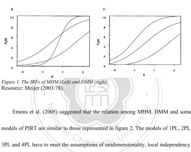
(49) Similarly, It can also imply to the ISRF in polytomous items (Emons et al., 2005; Hemker, 2000; Stochl, 2007).. Pi (θ ) ≥ P j (θ ), for all θ. (15). Models. The first model is referred to as the monotone homogeneity model (MHM). 政治大. (Mokken, 1971, 1997; Mokken & Lewis, 1982). MHM have to meet the first three. 立. assumptions, which are unidimensionality, local independency, and monotonicy. The. ‧ 國. 學. second model, referred to as the double monotonicity model (DMM), was developed. ‧. by adding the fourth assumption.. sit. y. Nat. n. al. er. io. Monotone homogeneity model. Ch. i Un. v. The model estimates the covariance among variables by nonparametric. engchi. regression (Meijer & Baneke, 2004; Ramsay, 2000). For polytomous items, the responses are represented by a set of ISRFs underlying the assumptions, which is all ISRFs of each item are monotonely nondecreasing (Molenaar & Sijtsma, 2000). The ISRFs of each item could intersect under MHM. The left side of figure 1 shows the form of MHM for dichotomous items. The model ranks the individual’s score by θ. That is, whoever has a higher score (X+) has a higher latent trait θ. The relation is. . 40.

(50) certain in dichotomous items, under the situation of polytomous analysis, the item steps of one item do not intersect. However, the ISRFs of different itemsare allowed to intersect (Molenaar & Sijtsma, 2000). Sijtsma and van der Ark (2001) and Sijtsma, & Molenaar (2002) suggested that it might be problematic in a small sample size for polytomous items.. P (X + ≥ χ + θ = θ a ) ≤ P (X + ≥ χ + θ = θ b ). 立. (16). 政治大. Double monotonicity model. ‧ 國. 學. The model not only has to fit the assumptions of undimesionality, local. ‧. independency, and monotonicity, but also reach the fourth assumption, which is the. y. Nat. al. er. io. sit. nonintersect of IRFs for dichotomous, and ISRFs for polytomous items of different. n. items (Molenaar & Sijtsma, 2000). The right side of figure 1 is the form of DMM for. Ch. engchi. i Un. v. dichotomous items. Under the model of DMM, the k items were ranked from easy to difficult. The easiest item is numbered as 1, the second easiest as 2, and the most difficult item is numbered as k. According to the numbered series, the conditional probability for a given ability to answer accurately would be shown as formula 17. For polytomous analysis, the ordering of the item step according to the. π gi , which. is defined by the difficulty of step i of item g, values is invariant. If the ISRFs of k polytomous items do not intersect, the items have an invariant ordering ( Molenaar & . 41.

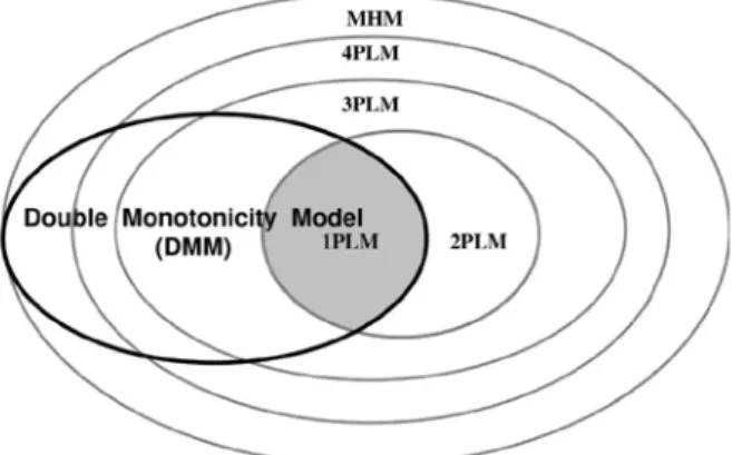
(51) Sijtsma, 2000). While the measurement of subjects is conducted by true-score scales, the difficulty of items is measured by the proportions scale (Meijer, 2003).. (17). P1 (θ ) ≥ P2 (θ ) ≥ ... ≥ Pk (θ ). 立. 政治大. ‧ 國. 學. Figure 1. The IRFs of MHM (Left) and DMM (right). ‧. Resource: Meijer (2003:78).. y. Nat. al. er. io. sit. Emons et al. (2005) suggested that the relation among MHM, DMM and some. n. models of PIRT are similar to those represented in figure 2. The models of 1PL, 2PL,. Ch. engchi. i Un. v. 3PL and 4PL have to meet the assumptions of unidimensionality, local independency, and monotonicy. In addition, they ascertain the assumptions by logistic IRF. That is, different to the models of NIRT. The DMM is a special case of MHM. Aside from the assumptions of MHM, DMM also has to fit the assumption of IIO.. . 42.

(52) Figure 2. The relation among the models of PIRT and NIRT. Resource: Emons, Sijtsma, and Meijer, (2005:105).. 立. 政治大. ‧. ‧ 國. 學. n. er. io. sit. y. Nat. al. . Ch. engchi. 43. i Un. v.

(53) 立. 政治大. ‧ 國. 學. This page intentionally left blank. ‧. n. er. io. sit. y. Nat. al. . Ch. engchi. 44. i Un. v.