國 立 交 通 大 學
機械工程學系
碩士論文
微壓電陀螺儀設計、分析與製作
Design and Fabrication of Duel Control Inputs Micro
Piezoelectric Gyroscopes
研究生 : 林奕帆
指導教授 : 陳宗麟 博士
微壓電陀螺儀設計、分析與製作
Design and Fabrication of Duel Control Inputs Micro
Piezoelectric Gyroscopes
研 究 生:林奕帆 Student:Yi-Fan Lin
指導教授:陳宗麟 Advisor:Tsung-Lin Chen
國 立 交 通 大 學
機 械 工 程 學 系
碩 士 論 文
A ThesisSubmitted to Department of Mechanical Engineering College of Engineering
National Chiao Tung University in partial Fulfillment of the Requirements
for the Degree of Master
in
Mechanical Engineering September 2013
Hsinchu, Taiwan, Republic of China
I
微壓電陀螺儀設計、分析與製作
學生:林奕帆
指導教授:陳宗麟 博士
國立交通大學機械工程學系 碩士班
中文摘要
本論文提出一平面設計之微壓電陀螺儀,此壓電陀螺儀在放置於待測物體上 和其驅動及感測模態皆設計在同一平面上,藉此去縮減音叉型和H型陀螺儀在固 定於待測物體上所占去的垂直體積。而驅動及感測材料採用壓電材料,正是看中 壓電材料結構簡單、輸出力大的優點去彌補微陀螺儀常見的因質量過小而造成響 應訊號之不足的問題。 在 ANSYS 軟體的模擬下,此論文提出的壓電陀螺儀設計驅動模態和感測模態 共振頻率分別在 4654 赫茲和 4674 赫茲;其操作頻率為 4664 赫茲。而在角速 度和輸出訊號間有一線性關係,並有 mini volt 數量級的輸出。對科氏力的估 算也有在此研究中提出,並且找出角速度、科氏力、位移量及訊號輸出間的關係。 文末提出兩種製程對於 PZT 在 Si3N4上沒有辦法結晶成功,以及非全 Pt 表 面上多層沉積結晶的不可行性進行了驗證,也提出製程替代方案,亦證實了製程 中因欲定義 SiO2 而在 PZT 無保護層的情況下使用濕式蝕刻程序的不可行性及提 供相關實驗數據,其他實驗相關數據,例如:PZT 蝕刻配方,蝕刻速率,每層沉 積厚度...等也都有提供,最後更提出 PZT 壓電材料裝置微機電製程流程方案。II
Design and Fabrication of Duel Control Inputs Micro
Piezoelectric Gyroscopes
Student: Yi-Fan Lin
Advisor:Dr. Tony Chen
Department of Mechanical Engineering
National Chiao Tung University
Abstract
This study proposes a piezoelectric gyroscope designed in a flat shape. The driving mode and detecting mode are on the same plane. Because of its flat shape, it will not occupy so much volume as the traditional fork-shaped and H-shaped gyroscopes in vertical space when it is installed on the target object. In addition, traditional gyroscopes face the problem of the detecting mass being too small, which causes output signals to be weak. Therefore, compared to traditional gyroscopes, using piezoelectric material for sensing and actuating would make the structure simpler and the signals of response will be much stronger.
In ANSYS simulations, the driving mode resonant frequency and sensing mode frequency are located individual at 4654 Hz and 4674 Hz. The operating frequency of this gyroscope is 4664 Hz. The relation between angular velocity and output signals is a linear tendency, and the signals were at the mini volt level. Coriolis force derivation is also mentioned in this study, and the relationships among angular velocity, Coriolis force, displacement and output electric potential are discussed.
In the last chapter, it is shown that the first fabrication process proved the unfeasibility of PZT multi-layer deposition on an incomplete Platinum layer surface and directly wet etches SiO2 without any protecting mask on the PZT layer. The
III
chapter includes data about the fabrication process, i.e. PZT etchant recipe, wet etching rate, PZT deposition thickness per layer etc. are provided too. At the end of the chapter, based on the unsuccessful fabrications, an improved fabrication process for PZT related device is proposed.
IV
Acknowledgement
此篇論文的完成,首先我要對我的父母獻上最高的謝意;在我求學生涯中, 您們沒有給我過多的壓力,總是無怨無悔的在我的背後支持我,而您們時刻的關 心著我的身心狀態,並給予我最大的關懷及溫暖,使我得以毫無後顧的完成學業。 真的很感激你們。 再來,在碩士求學過程中我非常感謝指導教授 陳宗麟老師;在研究過程中 不時的給予我方向及提供想法。而老師著重的學習精神及態度,雖然我在初期不 是很了解,但在和老師您不斷的溝通中,我才逐漸明白老師的用心良苦,在此我 獻上最高的敬意。 接著我要感謝身在遠方的朋友 緣庭,在這段生活中,妳總是給予我極大的 支持、鼓勵及包容,讓我總是可以在心情煩悶及研究不順遂時找到一些屬於自己 的空閒和時間去放鬆、充電和思考,使得我可以有足夠的動力持續下去,謝謝妳 不求回報的付出。 最後在研究和實驗上我要感謝學長,許齡元、蔡俊胤、張正暘無論是在研究 初期的構思給予思想上的幫助,或是到了後期實作階段的協助,這些都是完成此 論文的重要因素。而其他學長,吳健彰、張哲維、練瑞虔,還有同屆同學,李弘 輝、黃士維、吳承懋、王柏翔、曹修銓,以及其他實驗室學弟妹。是因為有你們 在,偶爾給予一些研究上的不同面向的思考,以及生活上的協助,才能使得此篇 論文得以順利完成,謝謝你們。V
Table of Contents
中文摘要 ···IAbstract ··· II
Acknowledgement ··· IV
Table of Contents ··· V
List of Table ··· VII
List of Figure ··· VIII
1
Introduction ··· 1
1.1 Outline of this Thesis ··· 1
1.2 Basic of Gyroscope ··· 1
1.3 Piezoelectric Material ··· 2
1.4 MEMS Fabrication Introduction ··· 3
2
Gyroscope ··· 5
2.1 Scientific Literature Review ··· 5
2.2 Introduction of Gyroscope ··· 6
2.2.1 Traditional Gyroscope ··· 6
2.2.2 Micro Gyroscope ··· 7
2.2.3 Piezoelectric Gyroscope ··· 10
2.3 Mathematic Model of Gyroscope ··· 13
3
Theory of Piezoelectric Material ··· 17
3.1 Conspectus of Piezoelectric Material ··· 17
3.2 Piezoelectric Constitutive Equations ··· 18
4
Design and Simulation Analysis ··· 22
VI
4.2 Harmonic Simulation Analysis ··· 31
4.3 Motion Simulation Analysis ··· 34
4.3.1 Displacement and Electric Potential Simulation ··· 34
4.3.2 Relation between Angular Velocity and Electric Potential ··· 36
4.3.3 Coriolis force simulation ··· 37
5 Fabrication Process ··· 41
5.1 Fabrication process ··· 41
5.2 Experiments of Fabrication ··· 41
5.2.1 First failed fabrication process ··· 41
5.2.2 Second failed fabrication process ··· 46
5.3 Fabrication process improvement ··· 51
6
Conclusion and Future work ··· 54
6.1 Conclusion ··· 54
6.1.1 Simulation analysis ··· 54
6.1.2 Fabrication process ··· 54
6.2 Future work ··· 55
VII
List of Table
Table 3.1: Parameters of piezoelectric ceramic (PZT-5) ··· 21
Table 4.1: Performance and resonating comparisons of different thickness ··· 29
Table 4.2: Performance and operation frequency of flat piezoelectric gyroscope ···· 30
Table 4.3: Displacements of 4 nodes on gyroscope arms ··· 32
Table 4.4: Displacement of 2 nodes by driving on feedback driving arm ··· 33
Table 4.5: Data of displacement of the end of detecting arm and electric potential ·· 36
Table 4.6: Angular velocity – Output voltage ··· 37
Table 4.7: Table of input voltage – displacement ··· 38
Table 4.8: Force – displacement chart ··· 39
Table 4.9: Relations of voltage, displacement and force on driving arm ··· 39
VIII
List of Figure
Figure 1.1: (a) Sagnac Interference;(b) Coriolis Effect ··· 2
Figure 1.2: Piezoelectric effects (a) Direct piezoelectric effect; (b) Conversely piezoelectric effect ··· 3
Figure 2.1: A simple two-axis gimbal set ··· 6
Figure 2.2: MEMS vibratory gyroscope ··· 8
Figure 2.3: Conceptual illustration of the Distributed-Mass Gyroscope with 8 symmetric drive-mode oscillators ··· 9
Figure 2.4: Structure schematic of linear vibration micro-gyroscope ··· 9
Figure 2.5: Beam-shaped piezoelectric gyroscope ··· 10
Figure 2.6: (a) Fork-shaped piezoelectric gyroscope (b) H-shaped piezoelectric gyroscope··· 11
Figure 2.7: Tri-fork-shaped piezoelectric gyroscopes ··· 12
Figure 2.8: Chart of mass in rotating frame and fixed frame ··· 13
Figure 4.1: Chart of gyroscope this study proposes ··· 22
Figure 4.2: Flat piezoelectric gyroscope ··· 23
Figure 4.3: Flat piezoelectric gyroscope working principle ··· 23
Figure 4.4: Input voltages on electrodes (PZT) ··· 24
Figure 4.5: Detecting part resonates in opposite phase··· 25
Figure 4.6: Flat piezoelectric gyroscope is driven and rotating at angular velocity 20 rad/sec. ··· 26
Figure 4.7: 10 vibration modes of gyroscope ··· 28
Figure 4.8: Detailed sizes of flat piezoelectric gyroscope ··· 30
Figure 4.9: Flat gyroscope is driven under operating frequency (4664 Hz) ··· 31 Figure 4.10: Driving on feedback driving arm under operation frequency (4664Hz) ··
IX
··· 33
Figure 4.11: Flat piezoelectric gyroscope undergo angular velocity 20 rad/sec and Coriolis force chart ··· 34
Figure 4.12: Bending arm chart ··· 35
Figure 4.13: Diagram of displacement – electrical potential ··· 36
Figure 4.14: Diagram of angular velocity – output voltage ··· 37
Figure 4.15: Nodes for observation ··· 38
Figure 5.1: Fabrication process I ··· 42
Figure 5.2: Steps for spin-coating PZT ··· 43
Figure 5.3: PZT sample by microscope ··· 44
Figure 5.4: Sample of PZT - I ··· 45
Figure 5.5: Sample of PZT - II ··· 46
Figure 5.6: Fabrication process II ··· 47
Figure 5.7: PZT surface plot by ET 4000 ··· 48
Figure 5.8: Sample of wet etching by BHF ··· 49
Figure 5.10: Experiment of PZT wet etching by BHF ··· 50
Figure 5.11: Comparison of 20sec etching sample and deeply hurt sample ··· 51
1
Chapter 1
Introduction
1.1 Outline of this Thesis
In Chapter 1, gyroscope, piezoelectric material and MEMS fabrications are briefly introduced.
Chapter 2 gives a deeper analysis of gyroscopes - its history, examples, as well as the derivation of gyroscope general motion equations.
In Chapter 3, Piezoelectric material’s history and classifications are described in section 3.1. The piezoelectric constitutive equation is introduced in section 3.2. It is used to describe piezoelectric material.
Chapter 4 analyzes the simulations of shape design, vibration modes, displacement, and electric potential. The relationships between displacement, electric potential, and angular velocity are also discussed in the chapter.
Two failed fabrication processes will be discussed in Chapter 5. The reasons for failure and experiments details will also be discussed. An improved fabrication process is proposed at the end of chapter 5.
Chapter 6 concludes the study and discusses future works.
1.2 Basic of Gyroscope
2
on the principles of the Sagnac effect and Coriolis effect.
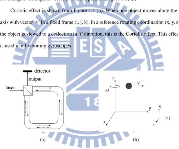
The Sagnac effect is also called Sagnac Interference. A beam of light is split, and the two beams are made to follow the same path, but in opposite directions. To act as a ring, the trajectory must enclose an area. On return to the point of entry the two light beams are allowed to exit the ring and undergo interference. The relative phases of the two exiting beams, and thus the position of the interference fringes, are shifted according to the angular velocity of the apparatus (Figure 1.1(a) ).
Coriolis effect is shown from Figure 1.1 (b). When one object moves along the j axis with vector ‘v’ in a fixed frame (i, j, k), in a reference rotating coordination (x, y, z) the object is viewed to a deflection in ‘i’ direction, this is the Coriolis effect. This effect is used in all vibrating gyroscopes.
(a) (b)
Figure 1.1: (a) Sagnac Interference;(b) Coriolis Effect
1.3 Piezoelectric Material
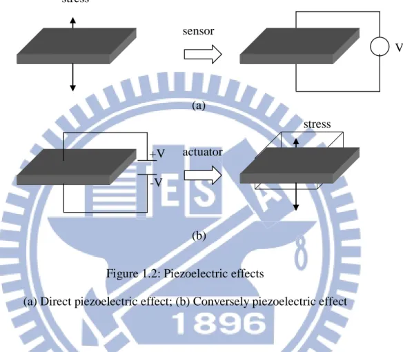
Piezoelectricity is an interaction between electrical and mechanical systems. Piezoelectric materials have two main effects. One is direct piezoelectric effect, and the other is converse piezoelectric effect. The direct piezoelectric effect is where
3
piezoelectric materials produce electric polarization by forcing mechanical stress (Figure 1.2 (a)). On the contrary, the conversely piezoelectric effect is when piezoelectric materials produce deformation by applying electric field.
Figure 1.2: Piezoelectric effects
(a) Direct piezoelectric effect; (b) Conversely piezoelectric effect
From these effects, the direct piezoelectric material and conversely piezoelectric effect can be used in the sensor and actuator respectively. A gyroscope is a device that combines the sensor and actuator in one, and hence piezoelectric material is suitable to be used.
1.4 MEMS Fabrication Introduction
Micro electro mechanical systems (MEMS) is the technology of very small devices. The fabrication of MEMS is from the process technology in semiconductor device fabrication, and the basic techniques are deposition of material layers, pattern
stress sensor V (a) actuator stress +V -V (b)
4
by photolithography and etching to produce the required shapes. MEMS technology, due to the advantages of being small in size and cheap in fabrication, has received more and more attention in specific applications.
5
Chapter 2
Gyroscope
2.1 Scientific literature review
There are two main fields in motion sensors, one is accelerometer, which is used for measuring speed changing, the other one is gyroscope used for measuring angular velocity. The first appearance of gyroscope can be tracked to the year 1852, Leon Foucault (1819-1868), a 19th-century French experimental physicist, who used the “gyroscope” apparatus to investigate the rotation of the earth. After that, along with the technologies advances, there are multiple variances in the development of gyroscopes. Gyroscopes have been extensively used to measure the angular velocity in many applications in our daily lives, such as vehicle navigation, vehicle rollover stability, digital camera image stabilization, and even in advanced military applications like aircrafts and satellites. In recent years, due to the regular need for better sensitivity, the development of gyroscopes are still in process and still attract attentions from the researchers in various fields. In addition, in order to the surge of virtual reality, and other applications as well, the development of gyroscope moves towards sensitive, reliable and miniature size for mass production.
According to their working principles, gyroscopes can be roughly classified to mechanical gyroscopes (rotor gyroscopes, vibratory gyroscopes… etc.) and optical gyroscopes (fiber gyros and laser gyros etc.). They all have theirs pros and cons and been utilized in various applications.
6
2.2 Introduction of Gyroscope
2.2.1 Traditional Gyroscope
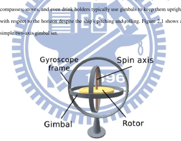
Gimbals is the basic of gyroscope, gimbals was first described by the Greek inventor Philo of Byzantium (280 – 220 BC) [1][2][3][4]. A gimbal is a pivoted support that allows the rotation of an object about a single axis. A set of three gimbals, one mounted on the other with orthogonal pivot axes, may be used to allow an object mounted on the innermost gimbal to remain independent of the rotation of its support (cf. vertical in the first animation). For example, on a ship, the gyroscopes, shipboard compasses, stoves, and even drink holders typically use gimbals to keep them upright with respect to the horizon despite the ship's pitching and rolling. Figure 2.1 shows a simple two-axis gimbal set.
Figure 2.1: A simple two-axis gimbal set
The first vibratory gyroscope was produced in early 1980s, it was made with quartz in fork-shaped. The basic idea of the vibratory gyroscope is that when the mass is oscillating along one axis (driving axis) and experiencing the angular velocity
7
simultaneously, the Coriolis force will produce a force along the axis (detecting axis) that is orthogonal to its original oscillating axis. Furthermore, the amplitude of the detecting axis is proportional to the applied angular velocity.
2.2.2 Micro Gyroscope
The first silicon MEMS gyroscope was produced in 1991 in Charles Stark Draper Laboratory; in the same year, a small vibratory piezoelectric gyroscope was made from Fujishima team [5]. After that, vibratory gyroscope became popular.
Compares to traditional mechanical gyroscope, the most characteristic of MEMS gyroscope is the micro size. Furthermore, in mass production, the cost is very low. However, because of the super mini size and the uncertainties in fabrications, these would cause a large influence to structure parameters, for instance, coefficient of elasticity, coefficient of dampness, oscillator mass… etc. Besides, defects in sensing circuits, such as, noise, parasitic capacitance, and non-idealities of amplifier… etc. All these will cause performance substantially be reduced. Hence, the most characteristics, micro-size, is also the most challenge of how to promote higher performance.
There are many methods by using electricity to drive gyroscope, electromagnetic, electrostatic, and piezoelectric …etc. Electromagnetic gyroscope could work in harsh environments, but it consumes power highly, further, the input circuit is so great that hard to control and not easily produce in MEMS fabrication, these made electromagnetic gyroscope can’t be used widely.
Electrostatic gyroscope generally measures values change of changeable capacities to estimate the oscillator mass deflection, which is caused from Coriolis force when it is rotating. The characteristics of consuming low power, stable, and input voltage is easy to be controlled. Yet, the extreme request of gaps accuracy and weak signal output are its biggest defects. Even though those defects, but the high
8
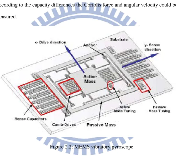
integrating with MEMS fabrication, it is still the most common type of MEMS gyroscope now. Figure 2.2 [6] shows an example of electrostatic MEMS vibratory gyroscope; the gyroscope needs an input signal to drive it under a fixed frequency to resonate it in drive direction, then when the device is in rotation, Coriolis force will push the active mass shifting along sense direction; and further, gaps distance in sense capacities, at two ends changed, then values of capacities will change lately. According to the capacity differences the Coriolis force and angular velocity could be measured.
Figure 2.2: MEMS vibratory gyroscope
Figure 2.3 [7] and Figure 2.4 [8] are another electrostatic MEMS vibratory gyroscopes, both they need an input signal at theirs designed resonating frequencies to oscillate the main masses to resonate along the driving axis, then when they are rotating, Coriolis force will cause the changing the values of changeable capacities, those comb-shaped structure. By counting the values, Coriolis force and angular velocity can be counted.
9
Figure 2.3: Conceptual illustration of the Distributed-Mass Gyroscope with 8 symmetric drive-mode oscillators
Figure 2.4: Structure schematic of linear vibration micro-gyroscope
Piezoelectric gyroscope has great output, responses fast and structure is uncomplicated, but piezoelectric materials performance is easily affected by
10
temperature and hard to produce in MEMS fabrication. So the purpose of this study is proposing a design with great output signals and can be combined with MEMS fabrication.
2.2.3 Piezoelectric Gyroscope
Piezoelectric gyroscope has many generations, but all principles are the same. Operator gives an input to oscillate main mass, when rotation occurs, Coriolis force cause transform on their structure, piezoelectric materials would produce corresponding electric signal output. Measuring the output can count the Coriolis force and angular velocity out.
The first generation is only like a beam (Figure 2.5) [9], oscillate in driving direction, when it is rotating, Coriolis force will curve it to the direction which is perpendicular to the driving direction, then by measuring the curving, then Coriolis force and angular velocity would be counted out. But there’s capacity effect due to the driving electrode is too close to the sensing electrode. Capacity effect means when two electrodes are charged, if they are too close, there will occur a capacity between two electrodes. This capacity will affect both electrodes and cause measuring errors. Besides, in this design the two modes, driving mode and sensing mode, are easily interfered by each others, this would made a huge error of output, hence fork-shaped gyroscope was proposed.
11
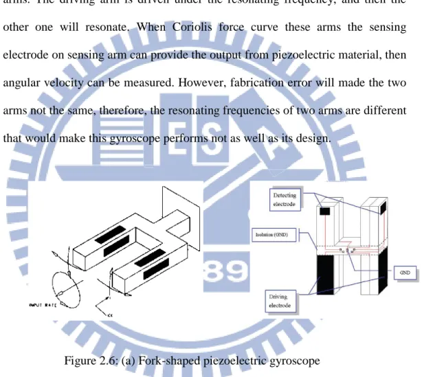
Fork-shaped gyroscopes (Figure 2.6(a)) [9], and its related version, H-shaped gyroscopes (Figure 2.6(b)) [10], are both important designs in vibratory gyroscope, in order to lower influence of capacity effect, fork-shaped gyroscope separates driving electrodes and sensing electrodes at two divided arms. The driving arm is driven under the resonating frequency, and then the other one will resonate. When Coriolis force curve these arms the sensing electrode on sensing arm can provide the output from piezoelectric material, then angular velocity can be measured. However, fabrication error will made the two arms not the same, therefore, the resonating frequencies of two arms are different that would make this gyroscope performs not as well as its design.
Figure 2.6: (a) Fork-shaped piezoelectric gyroscope (b) H-shaped piezoelectric gyroscope
H-shaped gyroscope is improved configuration since it can reduce the coupling effects between driving and sensing axis. For separating driving electrodes and sensing electrodes, the driving part is on top half and sensing part is at the other half to lower the electrostatic coupling and this symmetrical structure could also reduce the error from mechanical coupling. Wakatsuki [11][12] proposed the prototype of
12
H-shaped LiTaO3 Piezoelectric Gyroscope in 1997 and claimed that it had a better
ability to suppress the leakage couplings than that of the fork gyroscope. Moreover, the H-type vibratory gyroscope using LiTaO3 single crystal has large
electromechanical coupling coefficients, which can sharply suppress the “leakage” output. He also suggested that using a transducer attached to the driving axis to monitor and compensate the temperature drifting effect, which existed in most of the piezoelectric materials [13]. In 2001, an H-type gyroscope made of LiNbO3 with an
oppositely polarized single crystal plate had been reported [14]. Due to the electromechanical coupling factor of LiNbO3 is larger than that of LiTaO3 for the
flexural vibratory mode, this type of gyroscope is more suitable for miniaturization, due to the fact that they can produce the same amount of vibration amplitude in a more compact size, and achieving the same level of resolution.
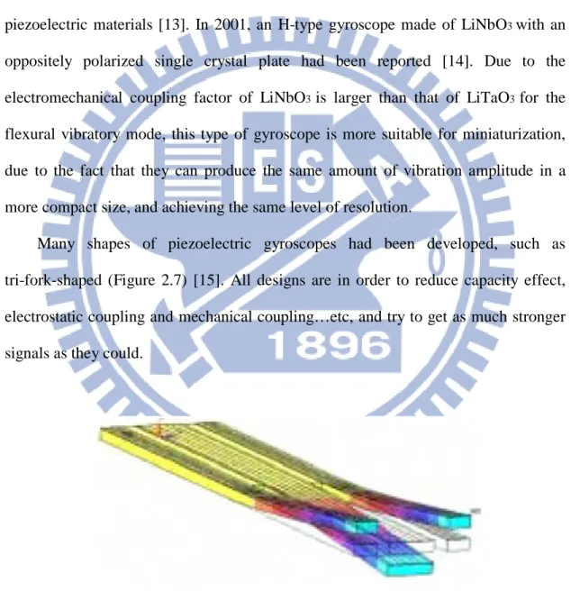
Many shapes of piezoelectric gyroscopes had been developed, such as tri-fork-shaped (Figure 2.7) [15]. All designs are in order to reduce capacity effect, electrostatic coupling and mechanical coupling…etc, and try to get as much stronger signals as they could.
13
2.3 Mathematic Model of Gyroscope
Coriolis acceleration could be counted out from relative motion equation as below.
Total force on mass (m) is below (relative to a rotating frame):
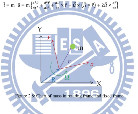
f⃑ = m ∙ a�⃑ = m �𝑑𝑑𝑡2𝑅�⃑2 + 𝑑2𝑟⃑ 𝑑𝑡2+ 𝑑𝛺��⃑ 𝑑𝑡 × 𝑟⃑ + 𝛺�⃑ × �𝛺�⃑ × 𝑟⃑� + 2𝛺�⃑ × 𝑑𝑟⃑ 𝑑𝑡� (2.1)
Figure 2.8: Chart of mass in rotating frame and fixed frame
Figure 2.8 shows a chart of a mass in rotating frame and fixed frame at the same time. The f �⃑ is total force on mass (m); a�⃑ is defined as the absolute acceleration of mass; the position vector 𝑅�⃑ is relative to rotating frame from fixed frame. Denoting the rotating frame by
F
for short; 𝑟⃑ is the position vector of mass relative toF
denoting by 𝛺�⃑ the angular velocity of theF
The first term in (2.1) is the linear acceleration ofF
relative to fixed frame, the second term is the linear acceleration of mass relative toF
, the third term is the linear acceleration of mass relative toF
, the fourth term is the centripetal acceleration of mass relative toF
, and the last term is14
called the complementary acceleration, or Coriolis acceleration, after the French mathematician de Coriolis (1792-1843), it’s also the value that gyroscope wants to measure. Notice that, on purpose of getting Coriolis acceleration, the last term in (2.1) must be existed, and the vector is cross product of angular velocity (𝛺�⃑) and the linear velocity (𝑑𝑟⃑
𝑑𝑡), of mass relative to
F
, hence Coiolis acceleration is vertical to bothterms.
If the terms of location vectors and angular velocity in (2.1) are replaced by Cartesian coordinates, it can be rewritten as:
{
F
} = {𝑒̂𝑥 𝑒̂𝑦 𝑒̂𝑧} (2.2) 𝑟⃑ = 𝑥𝑒̂𝑥+ 𝑦𝑒̂𝑦+ 𝑧𝑒̂𝑧 (2.3) 𝑑2𝑅�⃑ 𝑑𝑡2 = 𝑎𝑥𝑒̂𝑥+ 𝑎y𝑒̂𝑦+ 𝑎z𝑒̂𝑧 (2.4) Ω ��⃑ = Ω𝑥𝑒̂𝑥+ Ωy𝑒̂𝑦+ Ωz𝑒̂𝑧 (2.5)The (𝑥, 𝑦, 𝑧) is the location of the mass relative to
F
. The f �⃑ in (2.1) is assembled form spring structure, dampness and input. 𝑓 ���⃑ = 𝑓���⃑ + 𝑓𝑆 ����⃑ + 𝑓𝐷 ���⃑, and if (2.2) 𝐶 (2.3) (2.4) (2.5) also can be replaced by Cartesian coordinates as below:𝑓𝑆 ���⃑ = −𝑘1𝑥𝑒̂𝑥− 𝑘2𝑦𝑒̂𝑦− 𝑘3𝑧𝑒̂𝑧 (2.6) 𝑓𝐷 ����⃑ = −𝑑1𝑥̇𝑒̂𝑥− 𝑑2𝑦̇𝑒̂𝑦− 𝑑3𝑧̇𝑒̂𝑧 (2.7) 𝑓𝐶 ���⃑ = 𝑢𝑥𝑒̂𝑥+ 𝑢𝑦𝑒̂𝑦+ 𝑢𝑧𝑒̂𝑧 (2.8)
15
input.
Generally, mass of single-axis vibratory gyroscope is fixed on a plane. In this study, it assumes motion of the mass is restricted within x-y plane, but only detects the angular velocity on z-axis. In this assuming (2.1) can be rewritten into 2 axes dynamic equations by (2.2) (2.3) (2.4) (2.5) and (2.6) (2.7) (2.8):
m𝑎x+ mẍ + 𝑑1ẋ + �k1− m�Ωy2+ Ωz2�� x + m�ΩxΩy− Ω̇z�y = 𝑢𝑥+ 2𝑚Ω𝑧𝑦̇ (2.9)
m𝑎y+ mÿ + 𝑑2ẏ + �k2− m(Ωx2+ Ωz2)�y + m�ΩxΩy− Ω̇z�x = 𝑢𝑦− 2𝑚Ω𝑧𝑥̇ (2.10)
The two forces, 2𝑚Ω𝑧𝑥̇ and 2𝑚Ω𝑧𝑦̇ are resulted from Coriolis effect, from here, if wants the accuracy of angular velocity measuring more accurate the two Coriolis forces need to as greater as they can be. That depends on the mass and linear velocity. However the most characteristic of MEMS device is the micro-size, small size comes along with slight mass, about 10−6 ~ 10−8 kg. That also results in the difficulty of high accuracy of measuring.
Vibratory MEMS gyroscope used to be operated under the range of frequency from thousands to tens thousands hertz, hence the terms of angular velocities multiplying are far smaller than resonating frequency can be ignored. Therefore, (2.9) (2.10) can be simplified as:
mẍ + d1ẋ + k1x = ux+ 2mΩzẏ (2.11)
mÿ + d2ẏ + k2y = uy− 2mΩzẋ (2.12)
Equation (2.11) (2.12) describes single-axis gyroscope dynamic motions. From (2.11) (2.12), in ideality, there’s only dynamic coupling, in other words, excepting
16
itself rotation (Ωz≠0) gyroscope only affected by its own structure design, characteristics. Basic on this equation, angular velocity could be counted from dynamic coupling status.
17
Chapter 3
Theory of Piezoelectric Material
3.1 Conspectus of Piezoelectric Material
In 1824, Brewster found that tourmalines generate electrical charge when heated, or what is called “pyroelectricity”.
In 1880, the brothers Pierre Curie and Jacques Curie discovered piezoelectricity. They showed that crystals of tourmaline, quartz, and Rochelle salt (sodium potassium tartrate tetrahydrate) generated electrical polarization from mechanical stress.
There are many categories of piezoelectric material, and this study classifies them into 7 crystal systems and 32 point groups. 7 crystal systems include triclinic crystal system, monoclinic crystal system, orthorhombic crystal system, tetragonal crystal system, trigonal crystal system, hexagonal crystal system and cubic crystal system. Point groups are classified according to the structure and crystal symmetry. Crystal structure is directly related to piezoelectricity. For example, when one material is crystallized around a point of symmetry, the material is definitely not piezoelectric material. However, all non-center of symmetry point group, except for 432 point group, are piezoelectric materials. Now a widely used material, piezoelectric ceramics i.e. PZT, is a hexagonal crystal system and in the 6mm point group.
Piezoelectric ceramics are crystallized under high temperature. After polarization, it is like a single crystal with directionality. Another physical characteristic is the dielectric effect. When piezoelectric material is put in an electric field, electric charges are affected by the electric field and move, becoming electric dipoles, which
18
causes polarization - hence the dielectric effect. After that, under electric field or mechanical stress influences, piezoelectric materials generally will have a linear response.
Piezoelectricity is an interaction between electrical and mechanical systems. Piezoelectric materials have two main effects. One is direct piezoelectric effect, and the other is converse piezoelectric effect. The direct piezoelectric effect occurs when piezoelectric materials produce electric polarization by forcing mechanical stress on the material. On the contrary, the converse piezoelectric effect occurs when piezoelectric materials produce deformation by applying electric field on the material.
The electromechanical coupling effect of piezoelectric materials is used widely in engineering. With the two effects, many kinds of actuators and sensor can be made. However, there are some disadvantages worthy of concern in the application of piezoelectric materials. For example, it usually produces unnecessary coupling effects in any direction perpendicular to driving axis in the process of applying voltage.
In improving the accuracy and stability of piezoelectric devices, the null signal suppression of leakage couplings is significant. These null couplings have two main sources: mechanical and electromechanical couplings. The former is produced from manufacture defects, and the latter is because of the piezoelectric property between the driving and detecting electrode. These cases of leakage couplings can be improved either by changing the designed structure or dealing with control stratagems, in order to improve the resolution of the gyroscopes.
In general, piezoelectric materials have advantages of high strength, high bandwidth, short response time, and are used widely in vibratory gyroscopes.
19
Piezoelectric Constitutive Equation is described mathematically as below:
d-form:
�𝑆61(𝑇, 𝐸) = 𝑠66𝐸 𝑇61+ 𝑑63𝐸31
𝐷31(𝑇, 𝐸) = 𝑑36𝑇61+ 𝜀66𝑇 𝐸31 (3.1)
The four state variables (S, T, D, and E) can be rearranged arbitrarily to give an additional 3 forms for a piezoelectric constitutive equation by mathematics operation. It is possible to transform piezoelectric constitutive data from one form to another form. In addition to the coupling matrix d, they contain the other coupling matrices e,
g, or h in another 3 forms. What follows another 3 piezoelectric constitutive equations
and their mutual transformations:
e-form: �𝑇61(𝑆, 𝐸) = 𝑐66𝐸 𝑆61− 𝑒63𝐸31 𝐷31(𝑆, 𝐸) = 𝑒36𝑆61+ 𝜀66𝑆 𝐸31 (3.2) g-form: � 𝑆61(𝑇, 𝐷) = 𝑠66𝐷𝑇61+ g63𝐷31 𝐸31(𝑇, 𝐷) = −g36𝑇61+ 𝛽66𝑇 𝐷31 (3.3) h-form � 𝑇61(𝑆, 𝐷) = 𝑐66𝐷𝑆61− ℎ63𝐷31 𝐸31(𝑆, 𝐷) = −ℎ36𝑆61+ 𝛽33𝑆 𝐷31 (3.4) [𝛽𝑠] = [𝜀𝑆]−1, ℎ = 𝑘 𝑑2− 𝑑(1 − 𝑘𝑑2)−1 𝑠𝐷 = 𝑠𝐸(1 − 𝑘 𝑑2), 𝛽𝑇 = 𝜀1𝑇, g = 𝜀𝑑𝑇, 𝐶𝐸𝑆𝐸 = 1
20
T, S, E, D, d, g, h, 𝑘𝑑2 and e represent respectively stress, strain, electric field,
electric displacement, piezoelectric strain/coefficient of electric charge, piezoelectric strain/coefficient of voltage, piezoelectric stress/ coefficient of voltage, coefficient of mechanical-electric coupling and piezoelectric stress/ coefficient of electric charge. Those codes, such as 𝑠𝐸 with superscript means when the coefficient of function of S with constant variable E. 𝑠𝐷, 𝜀𝑇, 𝛽𝑇, 𝛽𝑠, 𝐶𝐸 represent respectively the coefficient of softness with constant electric displacement, coefficient of dielectric with constant stress, coefficient of converse dielectric with constant stress, coefficient of converse dielectric with constant strain and coefficient of stiffness with constant electric field.
In order to determine the piezoelectric material’s status, it needs 45 independent coefficients of material, but most piezoelectric materials have characteristic of symmetry in structure, so there are not as many coefficients as the hypothesis. The following diagram discribes piezoelectric ceramic as example, which is polarized in
3
x direction.
(3.5)
The T, D, S, E, 𝐶𝐸 in (3.5) are stress, electric displacement, strain, electric field and coefficient of stiffness with constant electric field respectively 𝜀𝑇, e, are
21
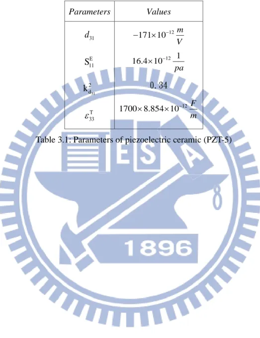
coefficients of dielectric and piezoelectric with constant strain. Table 3.1 shows parameters of PZT-5, which is also the material used in this study.
Parameters Values 31 d E 11 S 31 2 d k T 33
ε
12 171 10 m V − − × 12 1 16.4 10 pa − × 0.34 12 1700 8.854 10 F m − × ×22
Chapter 4
Design and Simulation Analysis
4.1 Shape Design and Vibration mode Analysis
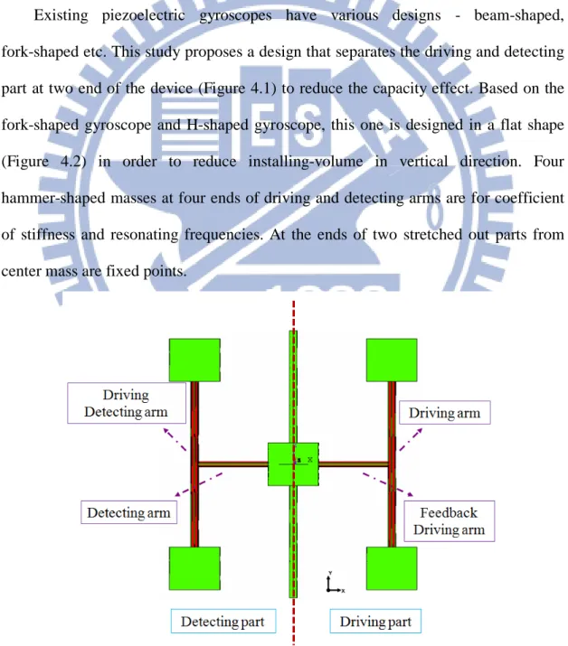
Existing piezoelectric gyroscopes have various designs - beam-shaped, fork-shaped etc. This study proposes a design that separates the driving and detecting part at two end of the device (Figure 4.1) to reduce the capacity effect. Based on the fork-shaped gyroscope and H-shaped gyroscope, this one is designed in a flat shape (Figure 4.2) in order to reduce installing-volume in vertical direction. Four hammer-shaped masses at four ends of driving and detecting arms are for coefficient of stiffness and resonating frequencies. At the ends of two stretched out parts from center mass are fixed points.
23
Figure 4.2: Flat piezoelectric gyroscope
This gyroscope uses piezoelectric effects to drive (Figure 4.3). When there is input of positive volt at the outer electrode (PZT) of the driving arm and negative volt at the inner electrode of the driving arm, the outer one will extend and the inner part will contract, then the driving arm will curve (Figure 4.4).
24
Figure 4.4: Input voltages on electrodes (PZT)
Meanwhile, if the gyroscope is driven under resonating frequency then the left half part will resonate in opposite directions (Figure 4.5).
25
Figure 4.5: Detecting part resonates in opposite phase
Furthermore, if the gyroscope is rotating around the Z-axis, then the detecting arm will curve (Figure 4.6) and then the deformation on detecting arm will make PZT electrodes output signals. Depending on the signals, Coriolis force and angular velocity can be measured.
In figure 4.1, the driving arm is for the driving input. The detecting driving arm is used to sense the amplitude of driving arm of being driven under resonating frequency. When the driving arm is driven under resonating frequency, the detecting driving arm will resonate in opposite direction with same amplitude. The detecting arm is for sensing. The feedback driving part will be introduced in section 4.2.
26
Figure 4.6: Flat piezoelectric gyroscope is driven and rotating at angular velocity 20 rad/sec.
After the prototype shape has been decided, vibration modes were close to being determined. Figure 4.7 shows 10 vibration modes. Sizes of every part are still important parameters to decide structure characteristics i.e. coefficient of stiffness, natural resonating frequency and performance etc.
27
Figure 4.7: (c) 1161 Hz Figure 4.7: (d) 1179Hz
Figure 4.7: (e) 1222 Hz Figure 4.7: (f) 2125Hz
28
Figure 4.7: (i) 4674 Hz Figure 4.7: (j) 5784 Hz Figure 4.7: 10 vibration modes of gyroscope
This study picks figure 4.7(h) and figure 4.7(i) as the driving and detecting mode respectively. As the driving mode and detecting mode resonating frequencies become much closer, the device will produce a greater signal output. These two modes resonating frequencies are 4654 and 4674, so the input frequency in this study used is 4664 Hertz.
Silicon makes up the whole structure, and compared to PZT thickness, the thickness of silicon affects performance much more. Table 4.1 shows the displacement when it is driven under operation frequency and its resonating frequencies. The displacement is an objecting point on driving arm, and this is a harmonic simulation with damping ratio 0.005.
The first row of table was the very first idea of design, and this table shows that the thicknesses of silicon and PZT does not affect resonating frequencies as much, but performance (the displacement of driving) is strongly affected by thickness of the silicion. In addition, it shows linear tendency. The thicker the silicon, the poorer the performance, while the thicker the PZT, the better the performance.
29
Table 4.1: Performance and resonating comparisons of different thickness
After a lot of tests and optimization of every part sizes, and taking into
consideration the cost, the final thickness and resonating frequency decided are shown in Table 4.2, the silicon basement is 300μm and PZT is 1.875μm.
Input voltage 20 ~ 0, 0 ~ -20 (Volt) Displacement at X-axis (m) Driving resonating frequency (Hz) Detecting resonating frequency (Hz) Operation Frequency
Silicon - 500 micro m, PZT- 25 micro m 7.06E-07 4749 4805 4777
Silicon - 500 micro m, PZT - 5 micro m 1.02E-07 4681 4837 4759
Silicon - 250 micro m, PZT - 5 micro m 2.90E-07 4705 4825 4765
Silicon - 250 micro m, PZT - 2.5 micro m 3.83E-07 4673 4821 4747
Silicon - 250 micro m, PZT - 1.25 micro m 3.55E-07 4662 4820 4741
Silicon - 250 micro m, PZT - 0.625 micro m 3.36E-07 4657 4821 4739
Silicon - 200 micro m, PZT - 1.25 micro m 4.65E-07 4665 4819 4742
Silicon - 200 micro m, PZT - 0.625 micro m 4.33E-07 4659 4820 4739.5
30
Table 4.2: Performance and operation frequency of flat piezoelectric gyroscope
Detail sizes are showed in figure 4.8:
Figure 4.8: Detailed sizes of flat piezoelectric gyroscope Input voltage 20 ~ 0, 0 ~ -20 (Volt) Displacement at X-axis (m) Driving resonating frequency (Hz) Detecting resonating frequency (Hz) Operation Frequency
31
4.2 Harmonic Simulation Analysis
In this study, harmonic simulation inputs a sinusoidal signal, which is within the resonating frequency to drive gyroscope. This section shows the extent of the deformation it could have. When the gyroscope is put it in a rotating frame, the experiment can also simulate how heavy the Coriolis force is and how much signal it can output.
Figure 4.9 was driven by a sinusoidal signal ranged from 20 ~ -20 volt:
32
The structure of design is on one side of wafer, and hence when it is operated, there may be structure deflection along out-plane axis caused by stress concentration.
Table 4.3 shows 3 axes displacements of 4 nodes in figure 4.9. In consideration of fabrication process, the PZT is only designed on one side, hence the unsymmetrical structure may cause z-axis deformation, so the displacement in z-axis is a key point needed to observe. Table 4.3 shows that the displacement in z-axis is much smaller than two other axes, thus this displacement is insignificant. Damping ratio here is 0.005
Node Ux (m) Uy (m) Uz (m)
29524 5.80963E-6 -3.26782E-7 1.31608E-9
34374 5.73231E-6 5.39366E-7 1.27389E-9
13634 -5.73259E-6 -5.38841E-7 1.13422E-9
17531 -5.80965E-6 3.27264E-7 1.04556E-9
Table 4.3: Displacements of 4 nodes on gyroscope arms
In figure 4.1 there is one part of the gyroscope named ‘feedback driving arm’, which is used for feedback driving. Because of its micro size, if the device undergoes a small velocity condition, the Coriolis force would be very weak, and in this condition, the feedback driving arm can be used. Input signal on the feedback driving arm can help the detecting arm reach the predicted amplitude, then, subtracting the amplitude from feedback input, the amplitude caused from Coriolis force can be derived. Figure 4.10 shows the diagram with 2 nodes that be observed.
33
Figure 4.10: Driving on feedback driving arm under operation frequency (4664Hz)
Table 4.4 shows displacement of 2 nodes in figure 4.10. Apparently, the displacements in y-axis of 2 nodes are almost the same, hence once the gyroscope is driven on feedback driving arm, the left part can resonate in opposite phase. In addition, displacements in z-axis are much smaller, so the displacement of z-axis can be ignored. Damping ratio here is 0.005.
Node Ux (m) Uy (m) Uz (m)
32907 2.63623E-9 -8.77733E-7 9.81261E-10
17827 -2.66178E-9 8.77252E-7 9.97343E-10
34
4.3 Motion Simulation Analysis
4.3.1 Displacement and Electric Potential Simulation
The harmonic simulation in section 4.2 without considering Coriolis effect, but in this section, Coriolis effect will be considered.
Figure 4.11 shows that, when gyroscope is driven on right arm then left arm will resonate in opposite phase, when it is in rotation frame (undergo angular velocity), Coriolis force will occur then bend detecting arm.
Figure 4.11: Flat piezoelectric gyroscope undergo angular velocity 20 rad/sec and Coriolis force chart
35
After Coriolis force bend the detecting arm, because of PZT electrodes deformation then they will output signals. Figure 4.12 shows that, when detecting arm is bended by Coriolis force, the PZT electrodes on detecting arm will deform. The below PZT electrode will extend a little bit and the one above will be contract slightly. Once deformation occurs, piezoelectric material will output electric signal. Hence according to the signals, Coriolis force and angular velocity can then be measured.
Figure 4.12; Bending arm chart
Because the bending curve quantity is small, it is assumed that the bending curve can be seen as linear displacement. Following Table 4.5 takes this assumption.
36
Figure 4.13 and table 4.5 show that, there is linear relation between displacement of the end of detecting arm and electric potential. Damping ratio here is 0.005:
Figure 4.13: Diagram of displacement – electrical potential
Voltage (v) 1.11E-04 2.22E-04 5.56E-04 1.11E-03 2.22E-03 5.56E-03 1.11E-02
Displacement
(m) 6.99E-09 1.40E-08 3.50E-08 6.99E-08 1.40E-07 3.50E-07 6.99E-07
Table 4.5: Data of displacement of the end of detecting arm and electric potential
4.3.2 Relation between Angular Velocity and Electric Potential
After determining the linear relation between deformation and output electric potential, it is important to find out the link between angular velocity and output voltage.
Table 4.6 shows voltage outputs of flat piezoelectric gyroscope undergo different angular velocities:
37
ω (°/sec) 1 2 5 10 20 50
Voltage
(volt) 1.11E-04 2.22E-04 5.56E-04 1.11E-03 2.22E-03 5.56E-03
ω (°/sec) 100 150 200 250 300 350
Voltage
(volt) 1.11E-02 1.67E-02 2.22E-02 2.77E-02 3.32E-02 3.87E-02
Table 4.6: Angular velocity – Output voltage
Figure 4.14 plots the table 4.6 data to a diagram:
Figure 4.14: Diagram of angular velocity – output voltage
Table 4.6 and figure 4.14 show the linear tendency between output voltage and angular velocity.
4.3.3 Coriolis force simulation
38
Coriolis force is. Hence this study tries to address this. In steady state condition, inputting a constant electric field on PZT will cause deformation. Table 4.7 shows the displacements of Node 29524 (Figure 4.15) by input different voltages on driving arm:
Figure 4.15: Nodes for observation
Input voltage (v) Node 29524 x-axis displacement (m) 0 0 1 -1.12E-08 2.5 -2.80E-08 5 -5.60E-08 7.5 -8.40E-08 10 -1.12E-07 15 -1.68E-07 20 -2.24E-07 30 -3.36E-07
39
Table 4.7: Table of input voltage – displacement
After that, a force is input on Node 29524 to match the displacement. Table 4.8 shows the conclusion:
Input force (N) Node 29524 x-axis displacement (m) 0 0 9.39E-05 -1.12E-08 2.35E-04 -2.80E-08 4.69E-04 -5.60E-08 7.04E-04 -8.40E-08 9.39E-04 -1.12E-07 1.41E-03 -1.68E-07 1.88E-03 -2.24E-07 2.82E-03 -3.36E-07
Table 4.8: Force – displacement chart
Tables 4.7 and 4.8 is combined into table 4.9:
Node 29524 x-axis Input voltage Displacement (m) Force/voltage N/V Input force Displacement (m) K- driving (N/m) 0 0 0 0
1 1.12E-08 9.39E-05 9.39E-05 1.12E-08 8.39E+03 2.5 2.80E-08 9.39E-05 2.35E-04 2.80E-08 8.39E+03 5 5.60E-08 9.39E-05 4.69E-04 5.60E-08 8.39E+03 7.5 8.40E-08 9.39E-05 7.04E-04 8.40E-08 8.39E+03 10 1.12E-07 9.39E-05 9.39E-04 1.12E-07 8.39E+03 15 1.68E-07 9.39E-05 1.41E-03 1.68E-07 8.39E+03 20 2.24E-07 9.39E-05 1.88E-03 2.24E-07 8.39E+03 30 3.36E-07 9.39E-05 2.82E-03 3.36E-07 8.39E+03
9.39E-05 N/V
40
Because the displacements are small, this study assumes the bending displacement can be seen as linear displacement, and according to basic hook’s law: 𝐹 = 𝑘𝑥, k is coefficient of stiffness, x is displacement, hence the coefficient of stiffness (K-driving, in table 4.9) of driving arm can be derived.
In the same way, the same process was done on Node 32907 then arranged data to table 4.10: Node 32907 y-axis Input voltage Displacement (m) Force/voltage N/V Input force Displacement (m) K- detecting (N/m) 0 0 0 0
1 1.19E-08 6.12E-05 6.12E-05 1.19E-08 5.13E+03 2.5 2.98E-08 6.12E-05 1.53E-04 2.98E-08 5.13E+03 5 5.96E-08 6.12E-05 3.06E-04 5.96E-08 5.13E+03 7.5 8.94E-08 6.12E-05 4.59E-04 8.94E-08 5.13E+03 10 1.19E-07 6.12E-05 6.12E-04 1.19E-07 5.13E+03 15 1.79E-07 6.25E-05 9.37E-04 1.79E-07 5.24E+03 20 2.38E-07 6.12E-05 1.22E-03 2.38E-07 5.13E+03 30 3.58E-07 6.12E-05 1.83E-03 3.58E-07 5.13E+03
6.13E-05 N/V
Table 4.10: Relations of voltage, displacement and force on detecting arm
Tables 4.9 and 4.10 show the coefficients of two arms, and the coefficient for the transformation between force and voltage. That means when detecting arm outputs a signal, it can be measured then transformed to an equal force, which is seemed apply on observing node. Therefore, the Coriolis force can then be measured.
41
Chapter 5
Fabrication Process
5.1 Fabrication process
The fabrication process will be discussed in this chapter step by step. During the fabrication process underwent changes twice because of unforeseen problems. The problems will also discussed in this chapter.
In order to simplify the process, PZT is only deposited on one side of silicon wafer, hence a single polished silicon wafer is used in this study. PZT is the actuating and detecting material, it is deposited by spin-coating [16] [17] [18] [19] [20] [21] [22] [23] [24] [25]. However, PZT is not an electric conductor, so it needs other metal layer as its electrodes. Platinum (Pt) is the most compatible candidate with PZT, and their crystal sizes are similar. As for electrodes, platinum has low electronic resistance, high melting point and high chemical stability. Because of the high chemical stability, that leads to challenges when patterning Pt by wet-etching, therefore, in order to pattern Pt, lift-off is used as the solution to this problem [25] [26]. Lift off process is a method of patterning of a target material on the surface of a substrate (ex. wafer) using a sacrificial material (ex. Photoresist). It is an additive technique as opposed to the more traditional subtracting technique like etching.
5.2 Experiments of Fabrication
5.2.1 First failed fabrication process
42
43
Figure 5.1: Fabrication process I
At very beginning, a layer of silicon nitrite is deposited by PECVD (plasma-enhanced chemical vapor deposition) as a seed layer, then a layer of photoresist(FH-6400L) is spin coated for lift-off, in order to pattern platinum (bottom electrode). Next 0.1μm thick platinum is evaporating deposited on it. Right after that, the whole wafer is dipped into acetone and an ultra sonic cleaner is used to remove photoresist. After these steps, the Pt is patterned on wafers.
The following chart shows the steps to spin coat PZT. (Figure 5.2):
Figure 5.2: Steps for spin-coating PZT
44
is to evaporate organic compounds. Baking at 700℃ is to crystallize PZT. The was smooth, but PZT layer was unable to function.
In figure 5.3, it is obviously can seen that, where the bottom is platinum (Pt), PZT could crystallize well on it, but apparently not on silicon nitride (Si3N4).
45
During the process, a main issue that surfaced is where PZT cannot be crystallized on a silicon nitride well, and cavities grow between the crystals. The rough surface then gradually grows and extends to a smooth surface (Figure 5.4). In the end, smooth surface will be covered by a rough surface. (Figure 5.5)
46
Figure 5.5: Sample of PZT - II
In this condition, the process definitely will fail, hence the fabrication process need to be changed.
5.2.2 Second Failed fabrication process
47
48
The core idea of the 2nd generation fabrication process is based the ease of PZT crystallizing on platinum. In the 2nd process, the Pt layer (bottom electrode) does not need to be patterned. The 1st process top electrodes and bottom are at the same layer, but once the bottom electrode is separated on the whole wafer surface in 2nd process, the top electrodes are needed to pattern on another layer. The study proposes an idea, which is depositing a silicon oxide (SiO2) layer on PZT to isolate the top Pt layer and
the bottom Pt layer.
The first few steps are retained - silicon nitride (Si3N4) is deposited by PECVD,
Pt is deposited by evaporative deposition, and PZT is deposited in the same steps by spin-coating. In addition, the PZT thickness per layer by the steps of spin-coating is about 0.075μm. Figure 5.7 is plotted by ET-4000, which is an instrument used for plotting surface sketch. The sample of PZT plotted by ET-4000 is spin-coated into 16 layers
Figure 5.7: PZT surface plot by ET 4000
The PZT etchant BHF* is BHF with other buffered solutions [27] [28] and the photoresist (PR) for protecting PZT from wet etching is AZ4620. The steps and recipe of PZT etchant is shown:
49
1. Etchant, BHF: HCI: NH4Cl: H2O = 1:2:4:4 (Volume ratio)
2. Dip in HNO3: H2O (2:1) solution for 10-15 secs
3. Immersing into DI water for 3- 5 mins
In this case, the average 1.2μm thick sample needs 55~60secs to be etched out, and the rate of etching is at about 0.02μm/sec and according to the experiment the undercutting ratio is almost 1:1.25 (Deepness : Sideness).
The next step is depositing silicon dioxide. It is deposited by PECVD for 0.5μm thick. After the step, patterning is done by wet etching. The etchant is BHF [29] [30]. The etchant is diluted 1:5. 0.5μm thick SiO2 is etched for 80~90 seconds. During the
wet etching process, BHF etches PZT layer as well( Figure 5.8).
Figure 5.8: Sample of wet etching by BHF
In order to confirm the etching rate of the etchant on PZT, A separate experiment was done to record the etching status every 10 seconds. (Figure 5.10)
50
Figure 5.10: Experiment of PZT wet etching by BHF
The surface of PZT is rough after undergoing wet-etching for over 20 seconds. In addition, the PZT sample is about 1.2μm. When it has been etched for about 60 seconds, almost all the PZT is gone, so the etching rate is about 0.02μm/sec. Compared to SiO2, 0.5μm thick silicon dioxide can bear about 90 seconds, and the
etching rate of SiO2 is about 0.005μm/sec.
BHF etches PZT more strongly than silicon dioxide. Figure 5.11 shows that after a few seconds, the PZT was unable to maintain its smooth surface. Over-etching is hard to avoid in the process of wet etching, but in this experiment, once that happens, BHF will hurt the surface of PZT. This would cause irreversible damage, hence this
51
process was also unsuccessful.
Figure 5.11: Comparison of 20sec etching sample and deeply hurt sample
5.3 Fabrication process improvement
After the above two unsuccessful processes, another improving fabrication process is proposed as below (Figure 5.12):
52
53
The PZT layer in this improved fabrication process is still deposited on Pt layer to keep it crystallizing well. Because of over-etching from 2nd process, in this process, another Pt layer is deposited as an etching mask before silicon dioxide is deposited. This Pt layer will be a protecting mask for the wet-etching of silicon dioxide.
54
Chapter 6
Conclusion and Future work
6.1 Conclusion
6.1.1 Simulation analysis
Various types of simulations have been analyzed in this study in chapter 4. As mentioned, flat shaped designs could help vertical volume to be minimized, and the difference of resonating frequency between driving mode and detecting mode are only 20Hz. In addition, the relationship between displacement-electric potential and angular velocity-output voltage are both linear tendencies. Most importantly, this gyroscope can still output 10−3 level volt output in small angular velocity condition. The coefficient of transfer between voltage and force is also derived.
The steps to derive Coriolis force are also described at the end of chapter 4. In simulations, this design should have many advantages.
6.1.2 Fabrication process
Although the first two fabrications were unsuccessful, they both still provided important fabrication information.
Firstly, even though silicon nitride is a delicate material, and is widely used as a seed layer in MEMS fabrication processes, but in this case, that would cause fabrication failure. Because of spin-coating PZT layer by layer, it would cause the rough part to extend to smooth parts in the end, which is mentioned in section 5.2. Hence, spin-coating PZT on the whole surface with Pt is the best defense against
55
fabrication process failure.
Secondly, these experiments were able to provide data on etching rates, and conclusions about the thickness of PZT per layer by spin coating and etchant recipes etc.
Thirdly, silicon dioxide has a strong ability of electric isolation, but in this case, the etchant, BHF, for silicon dioxide etches PZT much quicker than the target material, SiO2. Furthermore, wet etching is a common technique in MEMS
fabrications and over etching is unavoidable, therefore, if any fabrication needs to pattern SiO2 on PZT, they need to avoid wet etching silicon dioxide, if the SiO2 layer
is directly deposited on PZT.
Lastly, an improved fabrication of PZT related device for MEMS fabrication process is proposed.
6.2 Future work
This study had made some simulations, but if the factors in mathematics model can be determined, much more motion statuses can be predicted, and designing the control circuits would be useful to the field.
The design proposed in this study is a one side structure device. If the structure can be built on both sides of wafer, the performance can be double.
56
Bibliography
[1] Sarton, George. (1959). “A History of Science: Hellenistic Science and Culture
in the Last Three Centuries B.C.” New York: The Norton Library, Norton &
Company Inc. SBN 393005267. Page 349–350.
[2] Ernest Frank Carter: “Dictionary of Inventions and Discoveries”, 1967, p.74 [3] Hans-Christoph Seherr-Thoss, Friedrich Schmelz, Erich Aucktor: “Universal
Joints and Driveshafts: Analysis, Design, Applications”, 2006, ISBN
978-3-540-30169-1, p.1
[4] Robert E. Krebs, Carolyn A. Krebs: “Groundbreaking Scientific Experiments,
Inventions, and Discoveries of the Ancient World”, 2003, ISBN
978-0-313-31342-4, p.216
[5] S.E. Alper and T. Akin, “A Single-Crystal Silicon Symmetrical and Decoupled
MEMS Gyroscope on an Insulating Substrate,” Journal of
Microelectromechanical Systems, Vol. 14, No. 4, pp. 707-717, 2005
[6] A. M. Shkel, “Micromachined Gyroscopes: Challenges, Design Solutions, and Opportunities,” Smart Structure and Materials 2001, Proceedings of SPIE, Vol. 4334,pp. 74-85, 2001.
[7] Andrei M. Shkel、Cenk Acar、Chris Painter, Two Types of Micromachned
Vibratory Gyroscopes
[8] Shaohua Niu, Shiqiao Gao, Haipeng Liu, “Analysis and Design of Stiffness of the
Elastic Beam in Linear Vibration MEMS Gyroscope”
[9] Sid Bennett, Cleon H. Barker, Michael E. Ash, “Proposed IEEE Coriolis
Vibratory Gyro Standard and Other Inertial Sensor Standards”
[10] Chien-Ping Huang, “ Design and Controlof the H-type Piezoelectric Gyroscope
57
[11] Noboru Wakatsuki and Hiroshi Tanaka, “Finite Element Method Analysis of
Single Crystal Tuning Fork Gyroscope for Suppression of its Inner Leakage Coupling,” Jpn. J. Appl. Phys. Vol.36(1997) 3037-3040 Part 1, No. 5B, 30 May
1997
[12] Hiroshi Tanaka and Noboru Wakatsuki, “Electromechanical Coupling
Coefficients for a New H-Type LiTaO3 Piezoelectric Gyroscope,” Jpn. J. Appl.
Phys. Vol.37(1998) 2868-2871 Part 1, No. 5B, 30 May 1998.
[13] Mitsuharu Chiba and Noboru Wakatsuki, “Temperature Self-Compensated
Lithium Tantalate Piezoelectric Gyroscope for Higher Stability,” Jpn. J. Appl.
Phys. Vol.39 (2000) 3069-3072 Part 1, No. 5B, 30 May 2000.
[14] Keisuke Ono, Masanori Yachi1 and Noboru Wakatsuki, “H-Type Single Crystal
Piezoelectric Gyroscope of an Oppositely Polarized LiNbO3 Plate,” Jpn. J. Appl.
Phys. Vol. 40 (2001) 3699-3703 Part 1, No. 5B, 30 May 2001.
[15] YUKI IGA, KENSUKE KANDA, TAKAYUKI FUJITA, KOHEI HIGUCHI, KAZUSUKE MAENAKA, “A Design and Fabrication of MEMS Gyroscope
Using PZT Thin Films”
[16] J. Sun, M. Vittadello, E. K. Akdogan, A. Hall, N. Marandian Hagh, and A. Safari “Direct-Write Deposition of PZT Thick Films Derived from Modified Sol-Gel
Process”
[17] Guohong He, Christopher C T Nguyen, Jane C M Hui, S-W Ricky Lee and Howard C Luong “Design and analysis of a microgyroscope with sol–gel
piezoelectric plate”
[18] Xuan-Yu Wang , Chi-Yuan Lee , Cheng-Jien Peng , Pei-Yen Chend, Pei-Zen Changa “A micrometer scale and low temperature PZT thick film MEMS process utilizing an aerosol deposition method”
58
D Polla “Fabrication and structural characterization of a resonant frequency
PZT microcantilever”
[20] Tien-I Chang “Lead Zirconium Titanium Ceramics and Films Derived by the
Sol-Gel Process”
[21] 劉顯光 “Effect of additives on processing of PZT thick films”
[22] Chun-I Lin and Yung-Chun Lee “Fabrication of PZT Thick Film on
Platinum-Coated Silicon Substrate by an Improved Sol-Gel Deposition Method”
[23] 饒珮瑩”Design and Fabrication of A Miniature Piezoelectric Accelerometer by
MEMS Technology”
[23] 吳雋祥、余志成 “溶膠凝膠備製鋯鈦酸鉛薄膜製程與下電極材料對微加速計 性 能 的 影 響 ” 中 國 機 械 工 程 學 會 第 二 十 六 屆 全 國 學 術 研 討 會 論 文 集 E11-007
[24] H. Kozuka*, S. Takenaka, H. Tokita, M. Okubayashi “PVP-assisted sol-gel
deposition of single layer ferroelectric thin films over submicron or micron in thickness”
[25] H.D.Tong, R.A.F.Zwijze, J.W.Berenschot, R.J.Wiegerink, G.J.M.Krijnen, and M.C.Elwenspoek “Characterization of platinum lift-off technique”
[26] Hyung Suk Lee and Jun-Bo Yoon “A simple and effective lift-off with positive Photoresist”
[27] Kelu Zheng, Jian Lu, Jiaru Chu “Study on Wet-etching of PZT thin film”
[28] Kelu ZHENG, Jian LU and Jiaru CHU “A Novel Wet Etching Process of
Pb(Zr,Ti)O3 Thin Films for Applications in Microelectromechanical System”
[29] Kirt R. Williams, Kishan Gupta, Matthew Wasilik “Etch Rates for
Micromachining Processing—Part II”
[30] Kirt R. Williams, Richard S. Muller “Etch Rates for Micromachining Processing”