具聽音辨位和語音增強及辨識的唱歌機器人

國 立 交 通 大 學

機械工程學系

碩士論文

具聽音辨位和語音增強及辨識的唱歌機器人

Source Localization, Speech Enhancement and Recognition

of a Singing Robot

研 究 生: 桂振益

指導教授: 白明憲

具聽音辨位和語音增強及辨識的唱歌機器人

Source Localization, Speech Enhancement and Recognition

of a Singing Robot

研 究 生：桂振益

Student：Chen-Yi Kuei

指導教授：白明憲

Advisor：Ming-Sian Bai

國 立 交 通 大 學

機械工程學系

碩 士 論 文

A thesis

Submitted to Department of Mechanical Engineering

Collage of Engineering

National Chiao Tung University

in Partial Fulfillment of Requirements

for the Degree of

Master

in

Mechanical Engineering

June 2010

HsinChu, Taiwan, Republic of China

I

具聽音辨位和語音增強及辨識的唱歌機器人

研究生：桂振益 指導教授：白明憲 教授

國立交通大學 機械工程學系 碩士班

摘要

現今的機器人工業如雨後春筍般蓬勃發展，技術更是日新月異，各種功能的 機器人舉凡保全機器人、軍事機器人、居家看護機器人、娛樂機器人等琳瑯滿目， 而隨著社會水準以及人們對於生活品質要求的提高，娛樂機器人今日佔有相當重 要的地位。本論文提出了一種點唱機器人，會追蹤且同時轉到使用者的方向，所 以此點唱機器人必須具備聽音辨位及語音辨識的能力。其中聽音辨位的方法包括 以物體轉移函數為基礎的辨位方法和交互相關及廣義交互相關；語音辨識則在萃 取出特徵參數之後採用動態時軸校正的方法比對並且辨識。而為了要讓使用者命 令的聲音純化以提高辨識率，我們採用語音增強的技術，包括陣列訊號處理和以 相位差為基礎的語音增強方法。以上提及的演算法我們將擇其優者整合在樂高 NXT 機器人，而其操作平台為以 windows 為介面的資料擷取系統。

II

Source Localization, Speech Enhancement and Recognition

of a Singing Robot

Student: Chen-Yi Kuei Advisor: Ming-Sian Bai

Department of Mechanical Engineering National Chiao-Tung University

A

BSTRACT

Nowadays, there are a variety of functional robots included security robot, military robot, household robot and recreational robot, etc. With social progress and the attention of quality life, entertainment undertakings play an important role recently. In this thesis, we present a nickelodeon robot with simultaneous human-tracking. Therefore, the robot contains source localization and speech recognition techniques. The methods of source localization include object-related transfer function (ORTF) based, cross correlation (CC) and generalized cross correlation (CC) method. We recognize words by employing dynamic time warping (DTW) to do dynamic matching after feature extraction. For the purpose of increasing the purity of the command voice, we adopt speech enhancement which contains array signal processing and phase difference (PD) method. All algorithms we take the best one of each purpose to implement on the LEGO NXT robot controlled by windows-based NI DAQ system.

III

誌謝

時光飛逝，兩年碩士班研究生涯轉眼就過去了，首先感謝指導教授白明憲博 士的指導與教誨，使我順利完生學業與論文，在此致上最誠摯的謝意。而教授指 導學生時豐富的知識，嚴謹的治學態度以及追求學問的熱忱亦是學生的學習效法 的典範。 在論文寫作方面，感謝電機系冀泰石教授和電子系桑梓賢教授在百忙之中撥 冗並提出相當寶貴的意見，使得本論文的內容更趨於完善與充實，在此致上無限 的感激。 回顧這兩年的歲月，承蒙同實驗室的博士班林家鴻學長、李雨容學姐、陳勁 誠學長、劉志傑學長與在職博士班蔡耀坤學長、曾瑞宏學長及碩士班何克男學長、 艾學安學長、郭育志學長、王俊仁學長及劉冠良學長在研究與學業上的適時指點， 並有幸與同學廖國志、曾智文、張濬閣、陳俊宏、劉孆婷、廖士涵在研究上互相 討論，也感謝這兩年你們帶來的砥礪與笑聲。而與學弟徐偉智、王俊凱、吳俊慶、 衛帝安、許書豪、馬瑞彬的朝夕相處，亦是值得回憶。 最後僅將此論文獻給我親愛的家人。感謝我的父親桂建中先生總是無條件支 持我的決定，感謝母親馮志屏女士從小對我無微不至的呵護與諄諄教誨，感謝乾 媽馮志琴女士這麼多年來不求回報的付出，感謝姐姐桂萱蓉和弟弟桂睿廷平時的 打氣加油；感謝女友林吟盈總是陪在我身邊，聽我得意時的自吹自擂和在我失落 的時候給予安慰與鼓勵。要感謝的人實在太多不及備載，如有疏漏，在此也一併 致上最深的謝意。

IV

T

ABLE OF

C

ONTENTS 摘要 ... I ABSTRACT ... II 誌謝 ... III TABLE LIST ... V FIGURE LIST ... VI I. INTRODUCTION ... 1

II. SOURCE LOCALIZATION ... 3

2.1 ORIR-based method... 3

2.2 Cross correlation ... 5

2.3 Generalized cross correlation ... 8

2.3.1 Classical cross correlation ... 9

2.3.2 Smoothed coherence transform ... 9

2.3.3 Phase transform ... 10

III. SPEECH ENHANCEMENT ... 11

3.1 Array processing ... 11

3.2 Phase difference approach ... 14

IV. SPEECH RECOGNITION ... 17

4.1 Feature extraction... 17

4.2 DTW algorithm ... 18

V. SIMULATION AND EXPERIMENT ... 20

5.1 Source localization ... 20 5.2 Speech enhancement ... 21 5.3 Speech recognition ... 21 5.4 Robot implementation ... 22 VI. CONCLUSION ... 22 REFERENCE ... 25

V

T

ABLE

L

IST

VI

F

IGURE

L

IST

Fig. 1 Illustration of the DOA estimation problem in 2-dimensional space with two identical microphones: the source s k( ) is located in far-field, the incident

angle is θ, and the spacing between two sensors is d. ... 30

Fig. 2 (a) CCF, (b) GCCF of classical method, (c) GCCF of classical method of SCOT, (d) GCCF of PHAT method. ... 32

Fig. 3 Schematic diagram of filter-and-sum method. ... 33

Fig. 4 30-channel triangular filterbank. ... 34

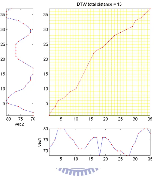
Fig. 5 The DP matching of two templates: the vertical axis stands for training speech template and the horizontal axis stands for test speech template. ... 35

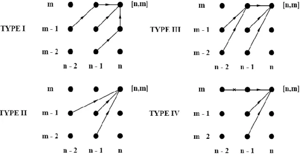
Fig. 6 Four kinds of local constraint for DTW. ... 36

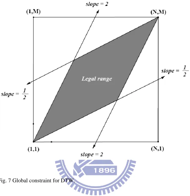
Fig. 7 Global constraint for DTW. ... 37

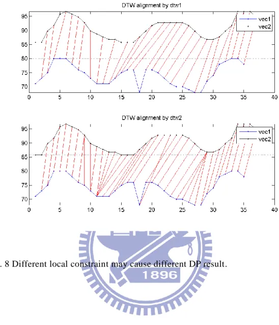
Fig. 8 Different local constraint may cause different DP result. ... 38

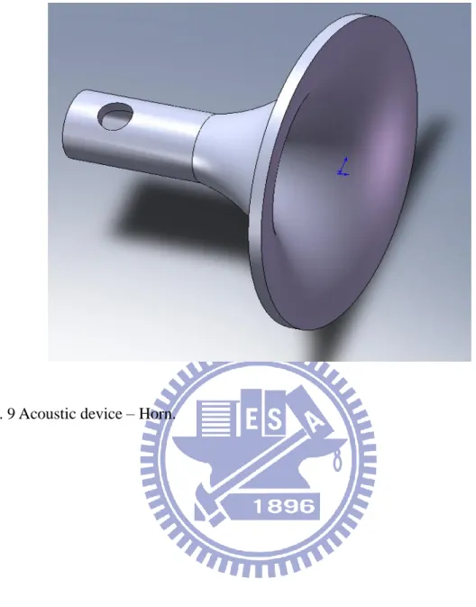
Fig. 9 Acoustic device – Horn... 39

Fig. 10 Robot system. ... 40

Fig. 11 Experimental configuration of ORIR measurement. ... 41

Fig. 12 (a) 0 degree ORTF, (b) 0 degree ORIR, (c) Magnified picture of (b). ... 42

Fig. 13 (a) 90 degree ORTF, (b) 90 degree ORIR, (c) Magnified picture of (b). .. 43

Fig. 14 (a) ITD database, (b) ILD database. ... 44

Fig. 15 (a) DOA estimation by CC method, (b) DOA estimation by GCC_PHAT method, (c) DOA estimation by hybrid method... 45

Fig. 16 (a) DOA estimation of 0 dB SNR noisy speech (white noise case) at different emitted angle, (b) DOA estimation of 12 dB SNR noisy speech (white noise case) at different emitted angle. ... 46

VII

Fig. 17 (a) DOA estimation of 0 dB SNR noisy speech (babble case) at different emitted angle, (b) DOA estimation of 12 dB SNR noisy speech (babble case)

at different emitted angle. ... 47

Fig. 18 (a) DOA estimation of 0 dB SNR noisy speech (exhibition case) at different emitted angle, (b) DOA estimation of 12 dB SNR noisy speech (exhibition case) at different emitted angle. ... 48

Fig. 19 (a) Beampattern of DAS, (b) Beampattern of maxDI, (c) Beampattern of constBW. ... 49

Fig. 20 (a) Waveforms of before DAS processing and after DAS processing, (b) Waveforms of before maxDI processing and after maxDI processing, (c) Waveforms of before constBW processing and after constBW processing, (d) Waveforms of before PD processing and after PD processing. ... 51

Fig. 21 RRs of clean speech polluted by white noise, babble, car noise and movie in different conditions of SNR. ... 52

Fig. 22 (a) RRs of polluted speech enhanced by DAS, (b) RRs of polluted speech enhanced by maxDI, (c) RRs of polluted speech enhanced by constBW, (d) RRs of polluted speech enhanced by PD. ... 54

Fig. 23 RRs of noisy speech (white noise case) at different emitted angle. ... 55

Fig. 24 RRs of noisy speech (babble case) at different emitted angle... 56

Fig. 25 RRs of noisy speech (exhibition case) at different emitted angle. ... 57

Fig. 26 Block diagram of whole system ... 58

1

I.

I

NTRODUCTION

Robot industry has developed and changed with each passing day. There are security robot [1], military robot [2], household robot [3] and entertainment robot [4], etc. However, Robot with function of karaoke, like a nickelodeon, is rarely seen. Now we present a robot which can turn to user and sing the song what user ask for. So, this nickelodeon robot has to localize the sound made by user and then recognize commands by speech recognition system. Because the environment can be noisy (i.e. the signal to noise ratio (SNR) is low), we combine with speech enhancement to purify command voice. Therefore, it comes three sub-topics: source localization, speech enhancement and speech recognition. Among these three sub-topics, source localization and speech enhancement are based on microphone array technology [5] [6]. We introduce these three sub-topics as follows:

Microphone array have received increasing attention in past few years, especially in spatial filtering (beamforming) [7], and source localization [8] [9]. Microphone array techniques depend on many factors, including placement, geometrical configuration, number of microphones, as well as the conditions and the number of active acoustic sources in the environment under investigation. Acoustic localization is an important task in many practical applications such as videoconferencing [10], hands-free communication system [11], hearing aids [12] and human-machine interaction [13]. Different kinds of source localization methods were proposed in the literature [5] [24]-[27]. In this thesis, we employ object-related impulse response (ORIR) based method, cross correlation (CC) and generalized cross correlation (GCC) [14] method. ORIR-based method is motivated by the algorithm based on head-related transfer function (HRTF) proposed by McDonald [15].

2

of using an array to enhance the desired signal reception while simultaneously suppressing the undesired noise can be easily illustrated by a delay-and-sum (DAS) beamformer [5]. To achieve better performance, we optimize the beampattern of microphone array [5]. On the other hand, our work in speech enhancement is to increase the words recognition rate (RR). It is well known that the human binaural system is remarkable in its ability to separate sound sources even in a very difficult environment. Motivated by these observations, many models and algorithms have been developed using interaural time difference (ITD), interaural intensity difference (IID), interaural phase difference (IPD), and other cues [16] [17] [18]. IPD and ITD have been extensively used in binaural processing because this information can be easily obtained by spectral analysis [16]. In this thesis, we only focus on the ITD cue and we construct a binary model to mask the undesired sound and extract the purpose speech without distortion.

The last part of this thesis is speech recognition. Currently, there are largely two types for recognizers – DTW-based and HMM-based method. DTW is a technique of dynamic programming (DP) –matching [19] [20]. DTW-based method suffers by speaker independent (SI) recognition cases whereas it shows good performance for speaker-dependent (SD) cases [21] [22]. Besides, DTW is suitable for less than 50 vocabularies work. On the Contrary, HMM-based method is utilized for large vocabulary and continuous speech recognition and can let everyone use after the training progress [23]. Nevertheless, DTW still has various applications including menu-driven commanding and phone dialing due to it is uncomplicated and easy to implement. In this thesis, we adopt DTW for our speech recognition because we only have only a few commands to be recognized.

3

based on ORIR, CC, and GCC method are involved. Section III introduces speech enhancement method such as array beamforming and phase difference (PD) algorithm. Section IV includes speech feature extraction and DTW algorithm. Some respective tests of the prior three sections and implementation of the singing robot are demonstrated in section V. The conclusion is provided in section VI.

II.

S

OURCE

L

OCALIZATION

2.1 ORIR-based method

Consider an array of m microphones mounted at arbitrary locations whose center is at point P. Imagine a sound that originates from azimuth  and elevation  relative to P. The task of any localization algorithm is to process each of the m microphone inputs { , ...,I₁ I_m} to generate azimuth and elevation estimates ˆ and ˆ, respectively. Ideally, the algorithm should utilize all available location cues to maximize accuracy. Differences in times of arrival between the microphones will vary with the location of the sound source and then can be utilized to generate location estimates. Additional location cues are available if the frequency content of the microphone inputs varies with the location of the sound source. This can be achieved by inserting an object centered at P into the listening environment so that the filtering properties of the object will vary with the orientation of the sound source.

For illustrative purposes, consider the situation in which m=2 microphones are mounted on the two sides of a robot. Let the center of the hearing system of the robot be located at P. Consider a sound that originates at azimuth  and elevation  relative to P. The sound is altered by the head and torso of the robot before it arrives at the microphones. If Ij is a digital recording of the input to the jth microphone,

4 then ( , ) * j j I O F   (1)

where O is the sound that would arrive at point P if the robot were absent, * is the convolution operator, and F_j( , )  is the object-related impulse response (ORIR) for

microphone j when a sound originates from ( , )  . The ORIR is a representation of the object-related transfer function (ORTF) in the time domain rather than the frequency domain and can therefore include both the time- and frequency-based filtering effects of the head and torso.

With the ORIR, the localization algorithm is motivated by the relationship of following two equations:

( , ) ( , ) ( , ) ( , ) ( , ) 1* 2 ( * 1 ) * 2 * 1 * 2 I F    O F   F   O F   F   (2) and ( , ) ( , ) ( , ) ( , ) ( , ) ( , ) ( , ) 2* 1 ( * 2 ) * 1 * 2 * 1 * 1 * 2 I F    O F   F    O F   F   O F   F   (3) This follows from the commutativity and associativity of the convolution operator. If the correct location is chosen, then the operation will lead to the same result for both microphone inputs. If the ORIR associated with some other location(  , ) is chosen, however, then the results will differ:

( , ) ( , ) ( , ) ( , ) ( , ) 1* 2 ( * 1 ) * 2 * 1 * 2 I F     O F   F     O F   F    (4) and ( , ) ( , ) ( , ) ( , ) ( , ) ( , ) ( , ) 2* 1 ( * 2 ) * 1 * 2 * 1 * 1 * 2 I F     O F   F    O F   F     O F    F   (5) Of course, a wide variety of similarity metrics are available; a moderate amount of testing suggested that the Pearson correlation maximized the accuracy and reliability of the “cross-channel” localization algorithm. Choosing ( , ) ˆ ˆ as follows:

5 ˆ ˆ ˆ ˆ ( , ) ( , ) 1 2 2 1 ˆ ˆ ( , ) m ax (r I *F   ,I *F   )   (6)

In advance, we measured the ORIR database



F1( , ),F2( , )



   

for doing the convolution operation in (6). Because we do not exactly know where the sound emits, we have to globally search ORIR database and then verify the correlation between

ˆ ˆ ( , ) 1* 2

I F   and I2*F1( , )ˆ ˆ  

. Ideally, if we make a correct choice, the Pearson correlation coefficient equals to 1. However, the coefficient can be affected by measurement accuracy, environment on the instant, quality of sound and so forth, we choose proximal one as estimated azimuth and elevation.

Even the “cross channel” approximation (i.e. finding the Pearson correlation coefficient which is most close to the value of 1) is directly perceived through the senses and accurate. But it is also computational consuming caused by global search. According to this drawback, we present a hybrid method. We utilize cross correlation (CC) and generalized cross correlation (GCC) method for roughly DOA estimation and then do the cross channel match for precision. Later on, we will introduce CC and GCC method.

2.2 Cross correlation

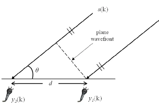
The DOA estimation is based on where the source is arranged to be in the array‟s far-field, as illustrated in Fig. 1. In this situation, sound source radiates a plane wave in the condition of propagating through the non-dispersive medium air. The normal to the wavefront makes an angle  with the line jointing the sensors in the linear array, so there exists time delay/advance between each microphone. In Fig. 1, we choose the right sensor as the reference point and the spacing between the microphones is denoted as d. Therefore, we can show that the plane wave needs more distance to get the second sensor. The distance can be easily calculated which

6

equals to dcos . So we know the time difference is given by ₁₂= cosd  /c, where c is the sound velocity in air. If the angle ranges between 0 and 180 and if _{1 2} is known then θ is uniquely determined, and vice versa. Therefore, estimating the incident angle θ is essentially identical to estimating the time difference

1 2

 . In other words, the DOA estimation problem is also called time-difference-of-arrival (TDOA) estimation problem in far-field case.

The speech source signal s k( ) propagates radiatively and the sound level drops as a function of distance from the source. If we choose the first microphone as the reference point, the signal received by nth microphone at time k can be expressed as follows: 1 ( ) ( ) ( ) [ ( )] ( ) ( ) ( ) , 1, 2, ..., n n n n n n n n n y k s k t k s k t k x k k n N                    (7)

where _n are the attenuation factors, s k( ) is unknown source signal, t is the

propagation time to sensor 1, _n( )k is an additive noise at the nth sensor, which is assumed to be uncorrelated with the signal and the noise captured by the other sensors,

 is the TDOA, and _n1 = _n( ) is the TDOA between sensor 1 and n with

1( )=0

  and  ₂( )= . For n = 3, … , N, the function _n depends only on 

because of the microphone array geometric. We have

( ) ( 1) , 2, ...,

n n n N

      (8) Consider only two microphones case, the cross-correlation function (CCF) between the two observation signal y k₁( ) and y₂( )k is defined as

7

1 2( ) [ 1( ) 2( )]

C C y y

r p  E y k y k  p (9)

Substituting (7) into (9) , we can get

1 2( ) 1 2 ( ) 1 2 ( ) 2 1 ( ) 1 2( )

C C C C C C C C C C

y y ss s s

r p   r p  r_ pt  r_ p t  r_{ } p (10) By the assumption of the signal and the noise are uncorrelated, (10) can easily checked that

1 2( )

C C y y

r p in Fig. 2 (a) reaches maximum at p . Hence, we can obtain the TDOA between y k₁( ) and y₂( )k as

1 2 C C ˆ arg m ax y yC C ( ) p r p   (11) where p [ _{m ax},_{m ax}], and _{m ax} is the maximum possible delay.

In digital implementation of (11), some approximations are required because of the CCF is not known and must be estimated. A normal practice is to replace the CCF defined in (9) by time averaged estimate. Suppose that at time instant k we have a set of observation samples of x_n, {x_n( ),k x_n(k1), ... ,x_n(kK 1)}, n1, 2, the corresponding CCF can be estimated as either

1 2 1 2 1 1 2 0 1 ( ) ( ) , 0 ( )= ( ) , 0 K p C C i y y C C y y y k i y k i p p K r p r p p            _{ } 



(12) or 1 2 1 2 1 1 2 0 1 ( ) ( ) , 0 ( )= ( ) , 0 K p C C i y y C C y y y k i y k i p p K p r p r p p          _   _{ } 



(13)

where K is the block size. The difference between (12) and (13) is that the former leads to a biased estimator, while the latter is an unbiased one. However, since it has a lower estimation variance and is asymptotically unbiased, the former had been

8

widely adopted in many applications.

2.3 Generalized cross correlation

Same as CC method, GCC employs free-field model (7) and considers only two microphones, i.e., N=2. Then TDOA estimate between the two microphones is obtained as the lag time that maximizes the CCF between the filtered signals of the microphone outputs which is often called the generalized CCF (GCCF):

1 2 C C ˆ arg m ax _{y y}C C ( ) p r p   (14) where 1 2 ˆG C C arg m ax _{y y}G C C( ) p r p   (15) 1 2 1 2 1 2 1 2 1 2 2 ( ) [ ( )] ( )e ( ) ( )e G C C y y y y j fp y y j fp y y r p F f f d f f f d f              





(16)

is the GCC function, F1[ ] stands for the inverse discrete-time Fourier transform (IDTFT), 1 2 * 1 2 ( ) [ ( )] y y f E Y Y f   (17) is the cross-spectrum with

2 ( ) ( ) j fk , 1, 2, n n k Y f 



y k e  n  (18) ( )f

 is a frequency-domain weighting function, and

1 2( ) ( ) 1 2

y y f  f y y

  (19) is the generalized cross-spectrum.

There are many different choices of the frequency-domain weighting function

( )f

9

2.3.1 Classical cross correlation

If we set ( )f 1, it can be checked that the GCC degenerates to the cross-correlation method, as seen in Fig. 2 (b). The only difference is that now the CCF is estimated using the discrete Fourier transform (DFT) and inverse discrete Fourier transform (IDFT), which can be implemented efficiently thanks to the fast Fourier transform (FFT).

We know from the free-field model (7) that

2 [ ( )]

( ) ( ) j f t n ( ) , 1, 2,

n n n

Y f  S f e    V f n  (20)

Substituting (20) into (19) and noting that the noise signal at one microphone is uncorrelated with the source signal and the noise signal at the other microphone by assumption, we have 1 2 2 2 1 2 ( ) [| ( ) | ] G C C j f y y f e E S f        (21) The fact that

1 2 ( )

G C C y y f

 depends on the source signal can be detrimental for TDOA estimation since speech us inherently non-stationary.

2.3.2 Smoothed coherence transform

In order to overcome the impact of fluctuating levels of the speech source signal on TDOA estimation, an effective way is to pre-whiten the microphone outputs before their cross-spectrum is computed. This is equivalent to choosing

2 2 1 2 1 ( ) [| ( ) | ] [| ( ) | ] f E Y f E Y f   (22)

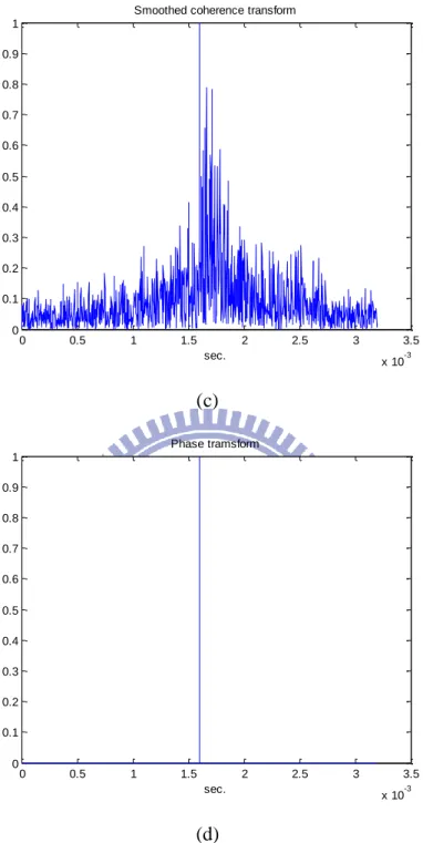
which leads to so-called smoothed coherence transform (SCOT) method [28]. Substituting (20) and (22) into (19) produces the SCOT GCC function and can be seen inFig. 2 (c):

10 1 2 1 2 2 2 1 2 2 2 1 2 2 2 1 2 2 2 2 2 2 2 1 1 2 2 2 1 2 [| ( ) | ] [| ( ) | ] [| ( ) | ] [| ( ) | ] [| ( ) | ] ( ) [| ( ) | ] ( ) 1 1 1 1 ( ) ( ) j f S C O T y y j f j f e E S f E Y f E Y f e E S f E S f f E S f f e S N R f S N R f                            (23) where 2 2 2 2 2 ( ) [| ( ) | ] [| ( ) | ] ( ) , 1, 2, [| ( ) | ] n n n n n f E V f E S f SN R f n E V f       (24) If the SNRs are the same at two microphones, then we get

1 2 2 ( ) ( ) [ ] 1 ( ) SC O T j f x x SN R f f e SN R f        (25) Therefore, the performance of the SCOT algorithm for DOA estimation would vary with the SNR. But when the SNR is large enough,

1 2 2 ( ) SC O T j f x x f e      (26) which implies that the estimation performance is independent of the power of the source signal. So, the SCOT method is theoretically superior to the CC method. But this superiority only holds when the noise level is low.

2.3.3 Phase transform

It becomes clear by examining (16) that the TDOA information is conveyed in the phase rather than the amplitude and only keep the phase. By setting

1 2 1 ( ) | ( )| y y f f    (27)

11 cross-spectrum is given by 1 2 2 ( ) P H A T j f y y f e      (28) which depends only on the TDOA τ. Substituting (28) into (19), we obtain an ideal GCC function: 1 2 2 ( ) , ( ) 0, P H A T j f p y y p f e df otherw ise     _{ }       _{ } 



(29)

The GCC function of PHAT is in Fig. 2 (d). As a result, the PHAT method performs in general better than CC and SCOT methods with respect to TDOA estimation.

III.

S

PEECH

E

NHANCEMENT 3.1 Array processing

In sensor arrays, a widely used signal model assumes that each propagation channel introduces some delay and attenuation only. With this assumption and in the scenario where we have an array consisting of N sensors, the array outputs, at time k, are expressed as

( ) [ ( )] ( ) ( ) ( ) , 1, 2, ...,

n n n n n n

y k  s k t F  v k x k v k 　　n N (30) where _n (n = 1, 2, . . .,N), which range between 0 and 1, are the attenuation factors

due to propagation effects, s(k) is the unknown source signal (which can be narrowband or broadband), t is the propagation time from the unknown source to sensor 1, v_n( )k is an additive noise signal at the nth sensor, τ is the relative delay or more often it is called the time difference of arrival (TDOA)] between sensors 1 and 2, and F_n( ) is the relative delay between sensors 1 and n with F₁( ) = 0 and

2( )

12

The most frequently and basically method that we use is delay-and-sum (DAS) beamformer. Such a beamformer consists of two basic processing steps. The first step is to time-shift each sensor signal by a value corresponding to the TDOA between that sensor and the reference one. With the signal model given above and after time shifting, we obtain , , , , ( ) [ ( )] ( ) ( ) ( ) ( ), 1, 2, ..., a n n n n a n a n a n y k y k F s k t v k x k v k n N           (31) where , ( ) [ ( )] a n n n v k  v k F  (32) and the subscript „a‟ implies an aligned copy of the sensor signal. The second step consists of adding up the time-shifted signals, giving the output of a DAS beamformer: , 1 1 1 ( ) ( ) ( ) ( ) N D S a n s s n z k y k s k t v k N   N 



   (33) where 1 , 1 1 1 , ( ) ( ) [ ( )] N s n n N N s a n n n n n N v k v k v k F          







(34)

Next, we introduce an optimized microphone array. In order to reject the noise in an acoustic field, we need to optimize the way we combine multiple microphones. Specifically we need to consider the direction gain, i.e. the gain of the microphone array in a noise field over that of a simple omni-directional microphone. A common quantity used is the directivity factor Q, or equivalently, the directivity index (DI) [10 log ( )₁₀ Q ].

13

The directivity factor is defined as

2 0 0 0 0 2 2 0 0 | ( , , ) | ( , , )= 1 | ( , , ) | ( , , ) sin 4 E Q E u d d                  

 

(35)

where the angle  and  are the standard spherical coordinate angles, ₀ and

0

 are the angles at which the directivity factor is being measured, E( , , )   is

the pressure response of the array, and u( , , )   is the distribution of the noise

power. The function u is normalized such that 2 0 0 1 ( , , ) sin = 1 4 u d d         

 

(36)

The directivity factor Q can be written as the ration of two Hermitian quadratic forms [35] as H H Q  w A w w B w (37) where 0 0 H  A S S (38)

w is the complex weighting applied to the microphones and H is the complex conjugate transpose. The elements of the matrix B are defined as

2 0 0 1 ( , , ) exp[ ( )] sin 4 m n m n b u j d d          

_{ }

k r r (39) and the elements of the vector S₀ are defined as

0n exp( 0 n)

s  jk r (40) Note that for clarity we have left off the explicit functional dependencies of the above equations on the angular frequency  . The solution for the maximum of Q, which is Rayleigh quotient, is obtained by finding the maximum generalized eigenvector of the homogeneous equation

14

M





A w B w (41) The maximum eigenvalue of above equation is given by

1 0 0 H M  _  S B S (42) The corresponding eigenvector contains the weights for combining the elements to obtain the maximum directional gain

1 0 o p t   w B S (43)

where w_{o p t} is our array filter with maximum directivity index (maxDI).

Besides, there is another type of optimization of array beampatterns: constant beamwidth (constBW). Its cost function is defined as

    1 2 2 0 0 2 2 0 0 , , sin 1 , , sin 4 H d d J H d d                  

 

 

(44)

We can also take above equation as a Rayleigh quotient problem which was mentioned before. Both maxDI and constBW are so called “filter-and-sum” technique which is shown in Fig. 3

3.2 Phase difference approach

For promoting speech recognition accuracy, we apply a two-microphone approach to extract the speech which is masked by other interference. The algorithm separates signals based on differences in arrival time of signal components from two microphones. As we know that the human binaural system is primarily based on the use of interaural time difference (ITD) at low frequencies and interaural level difference (ILD) information at high frequencies. However, we only focus on the use of ITD cues. When multiple sound sources are presented, it is generally assumed that humans only want to hear the sound from one direction which is equivalent to the

15

corresponding ITD.

First, the system performs a short-time Fourier transform (STFT) which decomposes the two input signals in time and in frequency. We get a subset of ITDs by comparing phase terms of the two input signals at each frequency. Through a time-frequency mask, we can extract the speech whose ITD is close to the target speaker and suppress unwanted sources.

The left-channel x n_L[ ] and right-channel x_R[ ]n are inputs of the system. We assume that the location of the desired target signal is known and its ITD is zero. For mathematical convenience, we refer to the number of interfering sources as L, with

( )l

 being their respective ITDs. Note that both L and ( )l

are unknown. With the above formulations, the signals are the microphones are

0 0 [ ] [ ] , [ ] [ ( )] L L L l R l t t x n x n x n x n  l   







 (45) with x n₀[ ] representing the target signal, x l_l(  0) representing interfering signals

L

x and x_R, respectively, representing the signals at the left and right microphones. The corresponding short-time Fourier transforms can be represented as

2 / ( , ) [ ] [ ] j kn N n X k m x n w m n e      



 (46) 0 2 ( , ) 0 ( , ) ( , ) ( , ) k i ( , ) L L i i L j d k m R i i X k m X k m X k m e  X k m     





(47)

where w n[ ] is a finite-duration Hamming window, k indicates one of N frequency bins, with positive frequency samples corresponding to _k 2 k

N    for 0 1 2 N k    .

In (45), the difference between two microphones is a pure time delay, but it is more appropriate to consider the time delays are function of frequency. Correspondingly,

16

we use the frequency-dependent ITD parameter d k m( , ) to replace the frequency-independent term  in (45). Next, we assume that a specific time-frequency bin (k₀,m₀), is dominated by a single sound source l. This leads to

* 0 0 0 * 0 0 0 , 0 ( , ) 0 0 0 , 0 ( ; ) ( ) ( ; ) k ( ) L l j d k m R l X k m X k m X k m e  X k m   (48)

where the source l* dominates the time-frequency bin(k₀,m₀). It becomes a simple binary decision to determine whether the time-frequency bin (k₀,m₀) belongs to the target speaker or not. The frequency-dependent ITD d k m( , ) for a particular time-frequency bin (k₀,m₀) is 0 0 , 0 0 0 0 0 1 | ( ) | m in | ( , ) | ( , ) 2 | | | r R L k d k m X k m X k m r      (49)

then we derive the binary masking criterion

0 0 0 0 1, | ( , ) | ( , ) , if d k m k m otherw ise         (50)

In other words, we take only time-frequency bins with the condition of

0 0

|d k( ,m ) | as the target speaker where  _{can be considered as width of}

receiving beam. And we use a small value 0.01 for  _{to block the unwanted} time-frequency bins. The mask ( ,k m) in (50) is applied to X k m( , ), the averaged signal spectrogram from the two channels, and speech is reconstructed from the

( , ) X k m where   1 ( , ) ( , ) ( , ) 2 ( , ) ( , ) ( , ) L R X k m X k m X k m X k m  k m X k m    (51)

17

The PD method illustrated above is based on the sound source is located in the direction of the microphone array axis (i.e. 90 degrees). In actual application, we can‟t guarantee that sound always originates at 90 degrees, so we employ beam-steering techniques [5] to compensate time delay between two sensors then do PD for speech enhancement. The beam-steering angle can be solved by DOA estimation which has been mentioned in section II.

IV.

S

PEECH

R

ECOGNITION

4.1 Feature extraction

In speech recognition system, we have to extract the characteristic of the signal as templates. In this thesis, we choose the commonly used Mel-frequency ceptral coefficient (MFCC) to be our speech feature. The Mel-frequency ceptrum is a representation of the short-term power spectrum of a sound. The difference from the real cepstrum is that a nonlinear frequency scale is used. Davis and Mermelstein [36] showed the MFCC representation to be beneficial for speech recognition. Next, we briefly introduce how this kind of parameter is extracted out.

First of all, given the DFT of the input signal

1 _{2 /} [ ] [ ] , 0 0 N _{j n k N} X k x n e k N a n   _      (52) Then, we design a filterbank with M filters (m=1, 2, … , M) , where filter m is triangular filter given by

0 [ 1] ( [ 1]) [ 1] [ ] ( [ ] [ 1]) [ ] ( [ 1] ) [ ] [ 1] ( [ 1] [ ]) 0 [ 1] m k f m k f m f m k f m f m f m H k f m k f m k f m f m f m k f m     _{ }  _{  }         _{  }        (53)

18 which satisfies 1 [ ] 1 M m m H k  



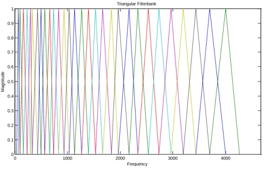
. As shown above, the frequency bands are equally spaced on the Mel-scale, which approximates the human auditory system‟s response more closely than the linearly-spaced frequency bands used in the normal cepstrum. These increasing bandwidths filters are displayed in Fig. 4. In (54), the boundary frequencies f m[ ] are calculated by the following equation:

1 1 1 ( ) ( ) [ ] ( ) [ ( ) ] 1 h s B f B f N f m B B f m F M      (54)

where the Mel-scale B and B-1 are defined as

1 ( ) 1 1 2 5 ln (1 ) 7 0 0 ( ) 7 0 0 [ex p ( ) 1] 1 1 2 5 f B f b B b       (55)

The input X_a[ ]k passed through each filter then we get the log-energy output

1 2 0 [ ] ln ( | [ ] | [ ] ) , 0 N a m k S m X k H k m M   



  (56) Finally, we take the discrete cosine transform (DCT) of the M filter outputs:

1 0 1 ( ) 2 [ ] [ ] co s( ) , 0 M m n m c n S m n M M     



  (57) where M varies from 24 to 40 in different kind of implementation. However, in speech recognition, we typically only use first 13 ceptrum coefficients.

4.2 DTW algorithm

DTW is based on overall distortion measure computed from the accumulated distance between the test and reference patterns along the aligned path. DTW is also called dynamic programming (DP) matching shown in Fig. 5. However, the alignment path is not apparent in the actual speech recognizers unless additional backtracking is performed.

19

The procedure for computing the accumulated distortion distance can be illustrated by the following procedure:

I)INITIALIZATION (1,1) (1,1), (1,1) 1, 2, ..., { (1, ) } D d B fo r j M co m p u te D j      II)ITERATION 1 1 2, ..., { 1, ..., { ( , ) m in [ ( 1, ) ( , )] ( , ) arg m in[ ( 1, ) ( p M p M fo r i N fo r j M co m p u te D i j D i p d p j B i j D i p d             , )] } } p j

III)BACKTRACKING AND TERMINATION

The optimal (minimum) distance is D N M( , ) _{and the optimal path is}

1 2

(s s, , ...,s_N)

where s_N  M and s_i  B i( 1,s_i1) , i  N 1,N 2, ...,1

For reducing the computation load and we consider that normal speaking speed cannot be more than two times of the training speed; therefore, we introduce two kinds of constraints: local constraint and global constraint. They can be expressed in Fig. 6 and Fig. 7, respectively. Fig. 8 shows different local constraint may cause different path to do the DP.

20

V.

S

IMULATION AND

E

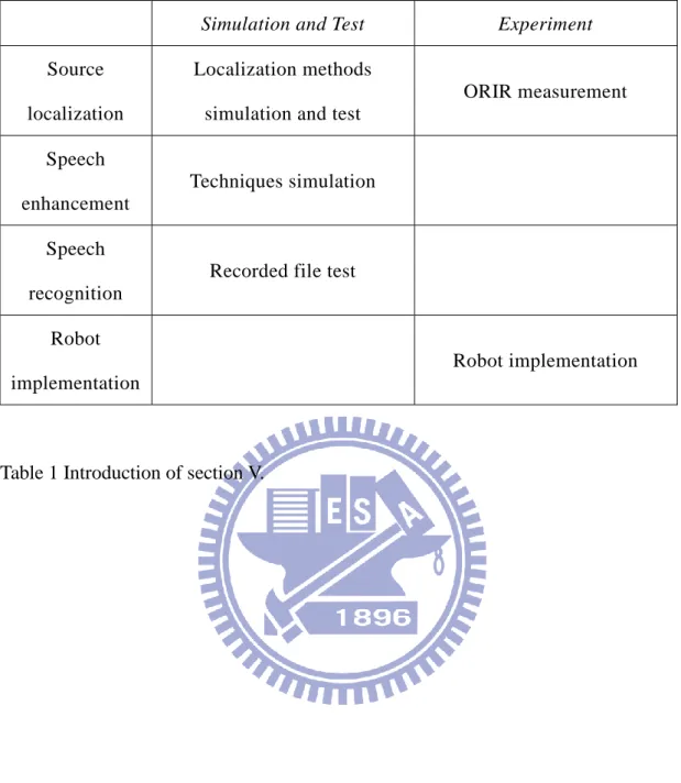
XPERIMENT

We divide this section into four parts: source localization, speech enhancement, speech recognition and finally, robot implementation. We give a briefly introduction which can be seen in Table 1.

In Table1, all the simulation and test are arranged by using two Knowles MEMS microphone (SPM0204HE5-PB) whose spacing is 0.05 m. However in experiment, our microphone spacing is changed by 0.2 m for increasing the resolution of the time delay estimation.

5.1 Source localization

First of all, we measure the ORIR from the test input (swept sine) to two sensors mounted on the LEGO NXT robot inside the 4m4m3m anechoic chamber. Besides, for increasing the directivity of the microphone array, we combine with an acoustic device – horn in Fig. 9. The robot system is displayed in Fig. 10.We utilize B&K Pulse audio analyzer (3560C) to generate signal and receive sound data, Tannoy loudspeaker (V8) to play test input, B&K power amplifier (2176) to magnify test input and B&K turntable system (9640) to rotate the robot for measuring sound from different azimuth. Fig. 11 gives the whole experimental configuration. Fig. 12 (a) shows the 0 azimuth ORTF, (b) is the ORIR, and (c) is the magnified picture of (b). Fig. 13 (a) shows the 90 azimuth ORTF, (b) is the ORIR, and (c) is the magnified picture of (b). Comparing with Fig. 12 (c) and Fig. 13 (c), we can clearly find that there exists time delay due to azimuth of the source. So we employ the CC method as mentioned before to compute the ITD. We gather ITD database and the azimuth is 5 degrees per move, from 0 degree to 355 degrees. Finally, we utilize 2-norm to calculate the ILD database. The ITD and ILD database can be seen in Fig. 14.

21

Secondly, we present some DOA estimation simulation result calculated by CC, GCC (PHAT) and hybrid method (GCC_PHAT combined with ORIR based method) in Fig. 15. Note that sound source emits from 90 degrees and noise emits from 30 degrees (SNR is 12 dB). By comparing the estimation results, we choose GCC_PHAT to be to construct hybrid method because it performs better than the others. Fig. 16 – Fig. 18 show that we use hybrid method (ORIR based method combines with GCC_PHAT) to do DOA estimation in the circumstance of sound source always emits from 90 degrees and 3 types of noise (white noise, babble and exhibition) emit from 0 degree to 75 degrees every 15 degrees (SNR is 0 dB and 12 dB).

5.2 Speech enhancement

First, we show the beampatterns of DAS, maxDI and constBW in Fig. 19. When we input a clean speech mixed with white noise and SNR is 10 dB, Fig. 20 (a) – (c) show the outputs passed through these three types of array and we compare them with the original input.

Secondly, we present the output passed through the PD and identically compare with the original output in Fig. 20 (d). It is easily seen that PD provides much better noise reduction performance than DAS, maxDI and constBW methods, so we just apply PD method on our experimental robot which will be later shown in section 5.4.

5.3 Speech recognition

In order to ensure that our speech enhancement works, we utilize the corpus provided by ITRI which concludes 50 commands in Mandarin made by 6 men and 5 women. After extracting features of each command, we apply DTW to do the DP-matching and recognize. In Fig. 21, we show that the clean speech polluted by white noise, babble, car noise and movie in different conditions of SNR. We set speech at 90 degrees and noise at 0 degree. The RRs of outputs enhanced by DAS,

22

maxDI, constBW and PD are shown in Fig. 22. By comparing Fig. 22, we can discover that PD performs significantly better than array processing.

Because PD provides better enhancement result, later we just employ PD method as our enhancement application. For detailed observation of the performance of PD, we set noise (white noise, babble and exhibition) every 15 degrees from 0 degree to 90 degrees and speech at 90 degrees always, the results are shown in Fig. 23 - Fig. 25. To achieve the best performance, we optimize  in (50) for each noise angle mentioned above.

5.4 Robot implementation

Fig. 26 shows block diagram of whole system. When two microphones mounted on the NXT robot receive the 2-channel signals, they are sent to source localization system and speech enhancement system. After the process of speech enhancement, signal is sent to speech recognition system. Now, we get the information of user‟s direction and speaking words. Finally, the robot turns to user and sings what user asks. Fig. 27 provides the schematic diagram of robot implementation.

VI.

C

ONCLUSION

The GCC methods are computationally efficient. They induce very short decision delays and hence have a good tracking capability: an estimate is produced almost instantaneously. We can also realize that GCC_PHAT has better performance than CC, classical GCC and GCC_SCOT in Fig. 2 because GCC_PHAT has the most obvious peak to make us find TDOA easily. Therefore, we only combine GCC_PHAT with ORIR-based technique to be our hybrid localization method. In Fig. 15, we can discover that hybrid method can catch the direction of target and interference more accurately than the others. Next we use this hybrid method to test numerous recorded

23

wave files. When the difference between angle of the target and angle of the interference is small, hybrid method still has the ability to distinguish them. But sometimes we may make wrong judgments when the noise is too loud (i.e. SNR is low).

Secondly, in Fig. 19 and Fig. 20 (a) – (c), we can discover that DAS, maxDI and constBW can only provide a little improvement because of the microphone number. If we use 4 microphones or more, the performance would be better certainly. PD exhibits it powerful ability to separate the desired voice from the interference and also provides excellent RR which will be demonstrated later.

Finally, we make a conclusion about speech recognition by analyzing the RR results. By comparing Fig. 21 and Fig. 22 (a) – (c), it is can be expectable that the RR gets insignificant promotion by array processing. However, we obtain remarkable RR result shown in Fig. 22 (d) when we utilize PD algorithm. We can control the value of

 to decide the angle of the receiving beamwidth. When we choose an appropriate

 which makes the target source pass through yet the interference be suppressed, we can get a purified signal without distortion. Therefore, the RRs can always be above 79% even at the situation of 0 SNR. In order to cope with all circumstances that the spanning angle between the purposed sound and the interference is not fixed. We put the interference at different azimuth. By our localization method and do a simple subtraction, we get the difference between angle of the target and angle of the main interference. By this, we can adjust  _{to optimize noise reduction performance.}

However, if the target sound and the interference originate from almost the same azimuth, we can‟t find any value of  to suppress unwanted noise which means PD method will fail in this case. It can be proved by Fig. 23 – Fig. 26. In Fig. 23 – Fig. 26, we set noise angle vary from 0 degree to 90 degrees and source angle always at 90

24

degrees. We can find that the RRs are above 58% except 90 degrees at 0 SNR. Unlike Fig. 22 (d), the RRs decrease because there exists DOA estimation error and leads to non-optimal  selection.

25

R

EFERENCE

[1] Luo, R.C. and Su, K.L. “Autonomous Fire-Detection System Using Adaptive Sensory Fusion for Intelligent Security Robot,” Mechatronics, IEEE, vol. 12, pp.274-281, June 2007.

[2] Voth, D., “A new generation of military robots,” Intelligent Systems, IEEE, vol. 19, pp. 2-3, Jul-Aug 2004.

[3] Krose, B., Bunschoten, R. Hagen ST, Terwijn, B., Vlassis, N., “Household robots look and learn: environment modeling and localization from an omnidirectional svision system,” Robotics & Automation Magazine, IEEE, vol. 11, pp. 45-52, Dec. 2004.

[4] Geppert, L, “Yoshihiro Kuroki: dancing with robots ,” Spectrum, IEEE, vol. 41, pp. 34-35, Feb. 2004.

[5] M. Brandstein and D. Ward, Microphone Arrays: Signal Processing Techniques

and Applications (Springer, New York, 2001).

[6] E. Hansler and G. Schmidt, Speech and Audio Processing in Adverse

Environments (Springer, New York, 2008)

[7] J. G. Ryan and R. A. Goubran, “Optimum near-field performance of microphone arrays subject to a far-field beampattern constraint,” J. Acoust. Soc. Am., vol. 108, pp. 2248-2255, 2000.

[8] J. C. Chen, R. E. Hudson, and K. Yao, “Maximum-likelihood source localization and unknown sensor location estimation for wideband signals in the near-field,”

IEEE Trans. Signal Process., vol. 50, pp. 1843-1854, 2002.

[9] X. Chen, Y. Shi, and W. Jiang, “Speaker tracking and identifying based on indoor localization system and microphone array,” 21st International Conference on

26

347-352, 2007.

[10] H. Wang and P. Chu, “Voice source localization for automatic camera pointing system in video conferencing,” Proceedings of the ICASSP, vol. 1, pp. 187-190, 1997.

[11] S. Fischer and K. U. Simmer, “An adaptive microphone array for handsfree communication,” Proceedings of the 4th International Workshop on Acoustic

Echo and Noise Control, IWAENC-95, pp. 44–47, 1995.

[12] M. R. Bai and C. Lin, “Microphone array signal processing with application in three-dimensional spatial hearing,” J. Acoust. Soc. Am., vol. 117, pp. 2112-2121, 2005.

[13] K. Nakadai, H. Nakajima, M. Murase, S. Kaijiri, K. Yamada, T. Nakamura, Y. Hasegawa, H. G. Okuno, and H. Tsujino, “Robust tracking of multiple sound sources by spatial integration of room and robot microphone arrays,”

Proceedings of the ICASSSP , vol. 4, pp. 929-932, 2006.

[14] C. H. Knapp and G. C. Carter, “The generalized correlation method for estimation of time delay,” IEEE Trans. Acoust., Speech, Signal Process., vol. 24, pp. 320–327, Aug. 1976.

[15] Justin A. MacDonald, “A localization algorithm based on head-related transfer functions,” J. Acoust. Soc. Am., vol. 123, pp. 4290-4296, June 2008.

[16] P. Arabi and G. Shi, “Phase-based dual-microphone robust speech enhancement,”

IEEE Tran. Systems, Man, and Cybernetics-Part B:, vol. 34, no. 4, pp.

1763-1773, Aug. 2004.

[17] D. Halupka, S. A. Rabi, P. Aarabi, and A. Sheikholeslami, “Real-time dual-microphone speech enhancement using field programmable gate arrays,”

27

March 2005.

[18] C. Kim, K. Kumar, B. Raj, and R. M. Stern, “Signal separation for robust speech recognition based on phase difference information obtained in the frequency domain,” INTERSPEECH-2009, Sept. 2009.

[19] Hiroaki Sakoe and Seibi Chiba, “Dynamic Programming Algorithm Optimization for Spoken Word Recognition,” IEEE Transcations on Acoustics, Speech, Signal

Processing vol. 26 (1), pp. 43-49, February, 1978.

[20] Hiroaki Sakoe and Seibi Chiba, “Comparative study of DP-pattern matchingtechniques for speech recognition” (in Japanese), in 1973 Tech. Group

Meeting Speech, Acoust. SOC. Japan, Preprints (S73-22),Dec. 1973.

[21] L. R. Rabiner and B. H. Juang, Fundamentals of Speech Recognition. Englewood Cliffs, NJ: Prentice Hall, 1993.

[22] C. Lévy, G. Linarès, and P. Nocera, “Comparison of several acoustic modeling techniques and decoding algorithms for embedded speech recognition systems,”

Workshop on DSP in Mobile and Vehicular Systems, Nagoya, Japan, Apr. 2003.

[23] Xuedong Huang, Alex Acero and Hsiao-Wuen Hon, Spoken Language

Processing, Prentice Hall PTR, NJ, 2001

[24] L. Wang, N. Kitaoka, and S. Nakagawa, “Robust distance speaker recognition based on position-dependent CMN by combining speaker-specific GMM with speaker-adapted HMM,” Speech Commun., vol. 49, 501-513, 2007.

[25] J. Benesty, “Adaptive eigenvalue decomposition algorithm for passive acoustic source localization,” J. Acoust. Soc. Am., vol. 107, 384-391, 2000.

[26] R. Bucher and D. Misra, “A synthesizable vhdl model of the exact solution for three-dimensional hyperbolic positioning system,” VLSI Des., vol. 15, 507-520, 2002.

28

[27] A. Brutti, M. Omologo, and P. Svaizer, “Speaker localization based on oriented global coherence field,” Proceedings of the Interspeech, pp. 2606-2609, 2006.

[28] G. C. Carter, A. H. Nuttall, and P.G. Cable, “The smoothed coherence transform,” Proc. IEEE, vol. 61, pp. 1497-1498, Oct, 1973.

[29] B. Champagne, S. Bédard, and A. Stéphenne, “Performance of time-delay estimation in presence of room reverberation,” IEEE Trans. Speech Audio

Process., vol. 4,pp. 148-152, Mar. 1996.

[30] J. P. Ianniello, “Time delay estimation via cross-correlation in the presence of large estimation errors, ” IEEE Trans. Acoust., Speech, Signal Process. ,vol. ASSP-30, pp.998-1002, Dec. 1982.

[31] M. S. Brandstein, “A pitch-based approach to time-delay estimation of reverberant speech,” in Proc. IEEE WASPAA, Oct. 1997.

[32] M. Omologo, and P. Svaizer, “Acoustic event localization using a crosspower-spectrum phase based technique,” in Proc. IEEE ICASSP, 1997, vol. 2, pp. 273-276.

[33] M. Omologo, and P. Svaizer, “Acoustic source location in noisy and reverberant environment using CSP analysis,” in IEEE ICASSP, 1996, vol. 2, pp. 921-924. [34] C. Wang and M. S. Brandstein, “A hybrid real-time face tracking system,” Proc.

IEEE ICASSP, 1998, vol. 6, pp. 3737-3741.

[35] D. K. Cheng, “Optimization techniques for antenna arrays,” Proc. IEEE, vol. 59, pp. 1664-1674, Dec. 1971.

[36] Davis, S. and P. Mermelstein, "Comparison of Parametric Representations for Monosyllable Word Recognition in Continuously Spoken Sentences," IEEE

29

Simulation and Test Experiment

Source localization

Localization methods simulation and test

ORIR measurement Speech enhancement Techniques simulation Speech recognition

Recorded file test Robot

implementation

Robot implementation

30

Fig. 1 Illustration of the DOA estimation problem in 2-dimensional space with two identical microphones: the source s k( ) is located in far-field, the incident angle is θ, and the spacing between two sensors is d.

31 (a) (b) 0 0.5 1 1.5 2 2.5 3 3.5 x 10-3 0 0.1 0.2 0.3 0.4 0.5 0.6 0.7 0.8 0.9 1 sec. Cross correlation 0 0.5 1 1.5 2 2.5 3 3.5 x 10-3 0 0.1 0.2 0.3 0.4 0.5 0.6 0.7 0.8 0.9 1 sec. Classical

32

(c)

(d)

Fig. 2 (a) CCF, (b) GCCF of classical method, (c) GCCF of classical method of SCOT, (d) GCCF of PHAT method. 0 0.5 1 1.5 2 2.5 3 3.5 x 10-3 0 0.1 0.2 0.3 0.4 0.5 0.6 0.7 0.8 0.9 1 sec.

Smoothed coherence transform

0 0.5 1 1.5 2 2.5 3 3.5 x 10-3 0 0.1 0.2 0.3 0.4 0.5 0.6 0.7 0.8 0.9 1 sec. Phase tramsform

33

34

Fig. 4 30-channel triangular filterbank.

0 1000 2000 3000 4000 0 0.1 0.2 0.3 0.4 0.5 0.6 0.7 0.8 0.9 1 Frequency M a g n it u d e Triangular Filterbank

35

Fig. 5 The DP matching of two templates: the vertical axis stands for training speech template and the horizontal axis stands for test speech template.

36

37

38

39

40

Fig. 10 Robot system.

Horn

Loudspeaker MEMS

41

Fig. 11 Experimental configuration of ORIR measurement. Tannoy V8

Loudspeaker

B&K 2716 Amplifier

B&K 3560C Pulse Audio Analyzer

B&K 9640 Turntable system

NB LEGO

42

(a)

(b)

(c)

Fig. 12 (a) 0 degree ORTF, (b) 0 degree ORIR, (c) Magnified picture of (b).

0 5000 10000 15000 20000 -60 -50 -40 -30 -20 -10 0 10 Frequency(Hz) M a g n it u d e (d B ) 0 degree left mic. right mic. 0 100 200 300 400 500 600 700 800 900 1000 -0.15 -0.1 -0.05 0 0.05 0.1 0.15 0.2 sample M a g n it u d e 0 degree left mic. right mic. 0 10 20 30 40 50 60 70 80 90 100 -0.15 -0.1 -0.05 0 0.05 0.1 0.15 0.2 sample M a g n it u d e 0 degree left mic. right mic.

43

(a)

(b)

(c)

Fig. 13 (a) 90 degree ORTF, (b) 90 degree ORIR, (c) Magnified picture of (b).

0 5000 10000 15000 20000 -60 -50 -40 -30 -20 -10 0 10 Frequency(Hz) M a g n it u d e (d B ) 90 degrees left mic. right mic. 0 100 200 300 400 500 600 700 800 900 1000 -0.25 -0.2 -0.15 -0.1 -0.05 0 0.05 0.1 0.15 0.2 0.25 sample M a g n it u d e 90 degrees left mic. right mic. 0 10 20 30 40 50 60 70 80 90 100 -0.25 -0.2 -0.15 -0.1 -0.05 0 0.05 0.1 0.15 0.2 0.25 sample M a g n it u d e 90 degrees left mic. right mic.

44

(a)

(b)

Fig. 14 (a) ITD database, (b) ILD database.

0 50 100 150 200 250 300 350 -40 -30 -20 -10 0 10 20 30 40 degree(s) sa m pl e( s) ITD 0 50 100 150 200 250 300 350 -15 -10 -5 0 5 10 sample(s) m ag ni tu de ILD

45

(a)

(b)

(c)

Fig. 15 (a) DOA estimation by CC method, (b) DOA estimation by GCC_PHAT method, (c) DOA estimation by hybrid method.

0 0.2 0.4 0.6 0.8 1 1.2 1.4 1.6 1.8 2 0 20 40 60 80 100 120 140 160 180 second de gr ee s DOA 0 0.2 0.4 0.6 0.8 1 1.2 1.4 1.6 1.8 2 0 20 40 60 80 100 120 140 160 180 second de gr ee s DOA 0 0.2 0.4 0.6 0.8 1 1.2 1.4 1.6 1.8 2 0 20 40 60 80 100 120 140 160 180 second de gr ee s DOA

46

(a)

(b)

Fig. 16 (a) DOA estimation of 0 dB SNR noisy speech (white noise case) at different emitted angle, (b) DOA estimation of 12 dB SNR noisy speech (white noise case) at different emitted angle.

47

(a)

(b)

Fig. 17 (a) DOA estimation of 0 dB SNR noisy speech (babble case) at different emitted angle, (b) DOA estimation of 12 dB SNR noisy speech (babble case) at different emitted angle.

48

(a)

(b)

Fig. 18 (a) DOA estimation of 0 dB SNR noisy speech (exhibition case) at different emitted angle, (b) DOA estimation of 12 dB SNR noisy speech (exhibition case) at different emitted angle.

49

(a)

(b)

(c)

Fig. 19 (a) Beampattern of DAS, (b) Beampattern of maxDI, (c) Beampattern of constBW.

50 (a) (b) 0 2000 4000 6000 8000 10000 12000 14000 16000 -1 -0.8 -0.6 -0.4 -0.2 0 0.2 0.4 0.6 0.8 1 sample m ag ni tu de DAS

before array processing after array processing

0 2000 4000 6000 8000 10000 12000 14000 16000 -1 -0.8 -0.6 -0.4 -0.2 0 0.2 0.4 0.6 0.8 1 sample m ag ni tu de maxDI

before array processing after array processing

51

(c)

(d)

Fig. 20 (a) Waveforms of before DAS processing and after DAS processing, (b) Waveforms of before maxDI processing and after maxDI processing, (c) Waveforms of before constBW processing and after constBW processing, (d) Waveforms of before PD processing and after PD processing.

0 2000 4000 6000 8000 10000 12000 14000 16000 -1 -0.8 -0.6 -0.4 -0.2 0 0.2 0.4 0.6 0.8 1 sample m ag ni tu de constBW

before array processing after array processing

0 2000 4000 6000 8000 10000 12000 14000 16000 -1 -0.8 -0.6 -0.4 -0.2 0 0.2 0.4 0.6 0.8 1 sample m ag ni tu de PD before PD after PD

52

Fig. 21 RRs of clean speech polluted by white noise, babble, car noise and movie in different conditions of SNR. 0 2 4 6 8 10 12 14 16 18 0 10 20 30 40 50 60 70 80 90 100 SNR R eco gn iti on R at e original white noise babble car movie

53 (a) (b) 0 2 4 6 8 10 12 14 16 18 0 10 20 30 40 50 60 70 80 90 100 SNR R eco gn iti on R at e DAS white noise babble car movie 0 2 4 6 8 10 12 14 16 18 0 10 20 30 40 50 60 70 80 90 100 SNR R eco gn iti on R at e maxDI white noise babble car movie

54

(c)

(d)

Fig. 22 (a) RRs of polluted speech enhanced by DAS, (b) RRs of polluted speech enhanced by maxDI, (c) RRs of polluted speech enhanced by constBW, (d) RRs of polluted speech enhanced by PD.

0 2 4 6 8 10 12 14 16 18 0 10 20 30 40 50 60 70 80 90 100 SNR R eco gn iti on R at e constBW white noise babble car movie 0 2 4 6 8 10 12 14 16 18 0 10 20 30 40 50 60 70 80 90 100 SNR R eco gn iti on R at e PD white noise babble car movie

55

Fig. 23 RRs of noisy speech (white noise case) at different emitted angle.

0 2 4 6 8 10 12 14 16 18 0 10 20 30 40 50 60 70 80 90 100 SNR R e co g n iti o n R a te white noise 0 degree 15 degrees 30 degrees 45 degrees 60 degrees 75 degrees 90 degrees

56

Fig. 24 RRs of noisy speech (babble case) at different emitted angle.

0 2 4 6 8 10 12 14 16 18 0 10 20 30 40 50 60 70 80 90 100 SNR R e co g n iti o n R a te babble 0 degree 15 degrees 30 degrees 45 degrees 60 degrees 75 degrees 90 degrees

57

Fig. 25 RRs of noisy speech (exhibition case) at different emitted angle.

0 2 4 6 8 10 12 14 16 18 0 10 20 30 40 50 60 70 80 90 100 SNR R e co g n iti o n R a te exhibition 0 degree 15 degrees 30 degrees 45 degrees 60 degrees 75 degrees 90 degrees