嵌入式系統低功率指令匯流排編碼方法

全文

(1)國立交通大學資訊工程系碩士論文. 嵌入式系統低功率指令匯流排編碼方法. Low-Power Instruction Bus Encoding for Embedded Systems. 研究生：陳彥銘指導教授：單智君博士. 中華民國九十四年八月.

(2) 嵌入式系統低功率指令匯流排編碼方法 Low-Power Instruction Bus Encoding for Embedded Systems. 研究生：陳彥銘. Student：Yan-Ming Chen. 指導教授：單智君. Advisor：Jean, J.J Shann. 國立交通大學資訊工程系碩士論文 A Thesis Submitted to Department of Computer Science and Information Engineering College of Electrical Engineering and Computer Science National Chiao Tung University in partial Fulfillment of the Requirements for the Degree of Master in. Computer Science and Information Engineering June 2005 Hsinchu, Taiwan, Republic of China. 中華民國九十四年八月.

(3) 嵌入式系統低功率指令匯流排編碼方法. 學生：陳彥銘. 指導教授：單智君博士. 國立交通大學資訊工程學系﹙研究所﹚碩士班. 摘. 要. 近年來如何降低嵌入式系統中的耗電量已經是個非常重要的課題了。對一般的嵌入式系統而言，系統耗電有相當顯著的比例是耗費在 off-chip 的匯流排上。匯流排上的耗電大約與其所傳送的資料位元變化量成正比，因此減少匯流排上的位元變化量是降低匯流排耗電的一個有效的方法。目前已經有許多減少位址匯流排耗電的研究被提出，然而減少指令匯流排耗電的編碼方法卻不多。在此，我們針對指令匯流排提出了一套編碼的方法，藉由減少指令匯流排上產生的電位變化而達成減少耗電的效果。利用 application-specific 的相關資訊，於 static time 將 hot-spots 中的指令轉換成做編碼並且利用表格記錄其編碼的資訊，讓處理器能於 dynamic time 時做解碼。實驗結果顯示，我們的方法能夠減少指令匯流排上 52%的耗電，比起 Petrov 提出的編碼方法約多出 16％的省電效果，比起 BIBIT 約多出 6％的省電效果。而且我們的硬體 overhead 與 BIBITS 約略相同而比 Petrov 的編碼方法小。整體而言，我們的研究可以帶來更好的省電效果。 -i-.

(4) Low-Power Instruction Bus Encoding for Embedded Systems. Student :Yan-Ming Chen. Advisors: Jean,J.J Shann. Department of Computer Science and Information Engineering National Chiao Tung University. ABSTRACT. Reducing the power consumption of embedded systems has gained a lot of research attention recently. In a typical embedded system, the power consumption in the off-chip buses consumes a great portion of the system power. Reducing the number of bit transitions is an effective way to reduce bus power since the bus power consumption is about proportional to the number of bit transitions. While many encoding techniques exist for reducing bus power in address buses, only a few have been proposed for instruction bus. For the low power requirement on instruction bus of embedded processors, we propose a bus encoding scheme to reduce power consumption on instruction bus. It exploits application-specific knowledge regarding program hot-spots, and identifies efficient instruction transformations to encode each instruction in hot-spots at static time. The few transformations that result in significant bit transition reductions for each hot-spot are selected by utilizing short indices stored into a table nearby the processor. The processor uses this information to efficiently restore the original bit sequence at dynamic time. The simulation results showed that our bus encoding can reduce the average power consumption of the bus by 52%, which is 16% more than Petrov’s bus encoding and 6% more than BIBITS. Moreover, the extra hardware overhead of our proposed is lower than Petrov's bus encoding and equal to BIBITS. We can conclude with certainly that our research may have more power saving opportunities.. -ii-.

(5) Table of Contents. ABSTRACT ..........................................................................................................ii Table of Contents .................................................................................................iii List of Figures ....................................................................................................... v List of Tables.......................................................................................................vii List of Tables.......................................................................................................vii Chapter 1. Introduction ...................................................................................... 1. 1.1. Importance of Low Power for Embedded Systems ....................... 1. 1.2. Power Consumption on Instruction Bus ........................................ 1. 1.3. Research Motivation ...................................................................... 3. 1.4. Research Goal ................................................................................ 4. 1.5. Organization of This Thesis........................................................... 4. Chapter 2. Background....................................................................................... 5. 2.1. Sources of Power Consumption..................................................... 5. 2.2. Previous Researches....................................................................... 7 2.2.1. BIBITS Bus Encoding...................................................................7. 2.2.2. Peter Petrov’s Instruction Bus Encoding.....................................11. 2.2.3. Summary of previous Researches................................................17 -iii-.

(6) Chapter 3. Design of Proposed Encoding ........................................................ 19. 3.1. Our Bus Encoding Scheme .......................................................... 20. 3.2. Hardware support......................................................................... 25. Chapter 4. Simulation and Analysis................................................................. 29. 4.1. Experimental Benchmarks ........................................................... 29. 4.2. Experimental Methods ................................................................. 30. 4.3. Experimental Toolset ................................................................... 30 4.3.1. Experimental Flow ......................................................................32. 4.3.2. Designing Experiments ...............................................................35. 4.4. Simulation Results and Analyses................................................. 35 4.4.1. Hardware Overhead Analysis......................................................36. 4.4.2. Bit Transition Reduction and Energy Saving of Our Encoding ..36. 4.4.3. Bit Transition Reduction of Different Techniques ......................38. 4.4.4. Bit Transition Reduction of Techniques with Different Transformation. Table Sizes...................................................................................................40. Chapter 5. Conclusion and Future Works ........................................................ 43. -iv-.

(7) List of Figures Figure 1-1 Architecture model of baseline system.....................................................................2 Figure 2-1: Design flow of BIBITS bus encoding scheme ........................................................8 Figure 2-2: BIBITS instruction partitioning...............................................................................9 Figure 2-3: BIBITS encoding example ....................................................................................10 Figure 2-4: Hardware support of BIBITS encoding.................................................................11 Figure 2-5: Design flow of Petrov’s bus encoding scheme......................................................12 Figure 2-6: Basic block partitioning example ..........................................................................13 Figure 2-7: Basic concept of Petrov’s encoding.......................................................................13 Figure 2-7: Petrov’s encoding example....................................................................................15 Figure 2-8: Petrov’s decoding example....................................................................................15 Figure 2-9: Hardware support of Petrov’s encoding ................................................................16 Figure 3-1: Design flow of our bus encoding...........................................................................19 Figure 3-2: Instruction partitioning example............................................................................21 Figure 3-3: Basic concept of our encodin.................................................................................22 Figure 3-4: Encoding example of our encoding scheme ..........................................................23 Figure 3-5: Decoding example of our encoding scheme..........................................................23 Figure 3-6: Function selection example ...................................................................................25 -v-.

(8) Figure 3-7: Decoder organization.............................................................................................26 Figure 3-8: Organization of each decoding component ...........................................................28 Figure 4-1: Experimental flow by using our experimental toolset...........................................34 Figure 4-4: Bit transition reduction of different techniques .....................................................39 Figure 4-5: Energy saving of different techniques ...................................................................39 Figure 4-6: mmul - Bit transition reduction with different transformation table sizes.............40 Figure 4-7: sor - bit transition reduction with different transformation table sizes..................40 Figure 4-8: jacobi - bit transition reduction with different transformation table sizes.............41 Figure 4-9: fft - bit transition reduction with different transformation table sizes...................41 Figure 4-10: tri - bit transition reduction with different transformation table sizes .................41 Figure 4-11: lu - bit transition reduction with different transformation table sizes .................42 Figure 4-12: Average bit transition reduction for full benchmarks with different transformation table sizes..................................................................................................................................42. -vi-.

(9) List of Tables Table 2-1: The 16 function of two Boolean variables ..............................................................14 Table 2-2: Comparison with transformation table size ............................................................18 Table 4-1: Benchmarks.............................................................................................................29 Table 4-2: Benchmark program size and numbers of each basic block ...................................30 Table 4-3: Experimental toolset descriptions ...........................................................................32. -vii-.

(10) Chapter 1. Introduction. First, we introduce why low power design is an important issue for embedded systems. And then we discuss why instruction bus consumes significant portion of system power. The research motivation and objective are then introduced. The organization of this thesis is described at last.. 1.1. Importance of Low Power for Embedded Systems The push for low power design has recently gained growing importance for embedded systems. In portable systems such as cellular phones and personal digital assistants (PDA), may severely undermine the usability and acceptance of the product by limiting its spatial and temporal range. Consequently, techniques for minimizing system power consumption are of significant importance for achieving high product quality.. 1.2. Power Consumption on Instruction Bus The ever-growing improvements in process technology have made system-on-chip (SoC) design attractive. A typical SoC design contains several embedded processor cores which are responsible for various parts of the total system functionality. Group of these embedded processors usually share on-chip or off-chip instruction memories containing the application code. The processor typically accesses these memories every cycle to fetch the next instruction. However, communicating instructions from memories to the processor front-end. -1-.

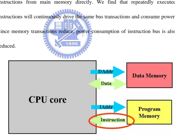
(11) relies on the utilization of long interconnect buses, which exhibit high capacitance. Therefore, the communication between a processor and its instruction memory significantly contributes to total power consumptions on the entire system. Having the instruction memory off-chip (for example, external flash memory) further aggravates this effect, because of the significantly higher capacitance of the bus lines going through the System I/O pins. Therefore, it is imperative to reduce power consumption on instruction bus. Figure 1-1 shows our baseline architecture model. At this baseline system, the processor sends address request and receives instructions from main memory directly. We find that repeatedly executed instructions will continuously drive the same bus transactions and consume power. Since memory transactions reduce, power consumption of instruction bus is also reduced.. Figure 1-1 Architecture model of baseline system. -2-.

(12) 1.3. Research Motivation Bus encoding is a general technique to reduce power consumption on bus by minimizing the switching activities per transition. As we mentioned in Section 1.2, reducing power consumption on instruction bus is an important research issue. While many bus encoding techniques exit for reducing bus power in address buses, only a few have been proposed for instruction bus power reduction.. Program memory data streams could be encoded at static time. Moreover, contents on bus transactions reflect program execution behaviors. It is a well-known property that programs typically spend most of their execution time within a relatively small part of the program code, such as loops. Such heavily executed program fragments are called as application hot-spots. A hot-spot may contain one or several basic blocks. During program execution, these basic blocks transmit on bus repeatedly. Therefore, if these frequently executed basic blocks can be transmitted with fewer bit transitions, power can be efficiently saved.. Previous low-power instruction bus encoding techniques either use a simple encoding scheme with limited transformation for encoding and decoding that bit transitions reduction is limited, or need a large table to store transformation information that the decoding power overhead is high.. -3-.

(13) 1.4. Research Goal In this thesis, we propose a low power encoding framework for embedded processor instruction buses. The encoder is capable of adjust its encoding not only to suit applications but furthermore to suit different aspects of particular program execution. It achieves this by exploiting application-specific knowledge regarding program hot-spots, and thus identifies efficient instruction transformations so as to minimize the bit transitions on instruction bus.. 1.5. Organization of This Thesis The remaining chapters of the paper are organized such that Chapter 2 introduces the source of power consumption, and discusses previous related researches on instruction bus encoding for power reduction. In Chapter 3, we describe our encoding techniques for instruction bus. The experimental environment, simulation results and relative analysis are presented in Chapter 4. Finally, we summarize our conclusions and future works in Chapter 5.. -4-.

(14) Chapter 2. Background. The main purpose of this chapter is to provide the necessary background for the concepts and methods presented in the following chapters. First, the main sources of power consumption in VLSI circuits based on static CMOS technology are introduced. Then, the chapter provides a survey of the related approaches for instruction bus power optimization and estimation appeared in the literature in the last few years.. 2.1. Sources of Power Consumption As CMOS processes scale to submicron dimensions, power associated with system buses and the I/O accounts for a large portion of the total system power consumption.. There are three major source of average power consumption in digital CMOS circuits which are summarized in the following equation: [1]. Pavg = Pswitching + Pshort−circuit + Pleakage 1 = α 0 →1C L ⋅ Vdd2 ⋅ f clk + I sc ⋅ Vdd + I leakage ⋅ Vdd . (1) 2 The first term represents the switching power which is due to the charge and discharge of the circuit node capacitances at the output of each logic gate, where CL is the load capacitance, Vdd is the supply voltage, fclk is the clock frequency and α0→1 is the node switching activity factor (the average number of times the node makes a power consuming transition in one clock period).The second is due to the direct-path short circuit current Isc which arises when both the NMOS and PMOS. -5-.

(15) transistors are simultaneously active, conducting current directly form supply to ground. Finally, leakage current Ileakage, which can arise from substrate injection and sub-threshold effects, is primarily determined by fabrication technology considerations. However, in “well-designed” CMOS devices, leakage power consumption can be considered insignificant in most designs [2].. The dominant term is the switching power and low-power design thus becomes the task of minimizing α0→1 , CL , Vdd ,and fclk. Factor CL is decided once the manufacture process has been chosen. Decreasing the Vdd factor has a quadratic effect and can be an effective way. However, the supply voltage is usually determined by the system and technology consideration, and decreasing Vdd will accordingly increase the propagation delay. By reducing the factor fclk, clock frequency, the computing time will be definitely extended. A multitude of techniques for scaling voltage or frequency have been proposed [3][4].. Another important factor that distinguishes power is its dependence on the switching activity. There are two ways to cut-down the switching activity on buses in execution time:. 1. Reducing transaction counts: Reducing requests of memory access is a direct approach to reduce bit transitions on buses. Since requests are saved, buses can keep idle and eliminate power. -6-.

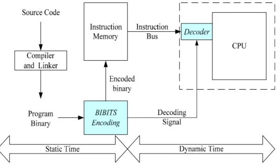
(16) consumption. To increase the reusability of transmitted values is a common example of this idea.. 2. Reducing number of switch activities per transaction: Reducing number of switch activities per transaction that make the current transmitted bits near previous ones can reduce number of capacitances needed to be driven. Bus encoding is a well-known technique to encode the content of bus to reduce the switching activities.. 2.2. Previous Researches Two previous researches for low power instruction bus encoding to reduce bit transitions are introduced in the following sections: BIBITS [5] and Petrov’s encoding scheme [6].. 2.2.1. BIBITS Bus Encoding BIBITS encoding shown in Figure 2-1 is to reduce the bit transitions on instruction bus. This encoding concentrates the effort on the application hot-spots and encodes the instructions at static time. The encoded instructions reside in the program memory, and the processor core receives information about transformation residing in additional table nearby the processor, either when loading the program or when running the software. The processor’s fetch module uses this information to efficiently restore the original bit sequence at dynamic time.. -7-.

(17) Figure 2-1: Design flow of BIBITS bus encoding scheme The design issues of BIBITS encoding are instruction partitioning and encoding function selection. The objective of these design issues is to use the most suitable encoding functions for different instruction partitions.. An instruction is partitioned into fields according to its format. Using the MIPS instruction formats as an example, an instruction is partitioned as in Figure 2-2. All register fields become individual partitions; bit 6 and 30 are in one partition and not to be encoded since they cause bit transitions relatively infrequently, and all the other partitions are in 5-bit groups.. -8-.

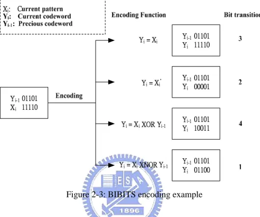
(18) MIPS Instruction Formats R. op. rs. rt. I. op. rs. rt. J. op. rd. shamt. funct. 16 bit address 26 bit address. Instruction Partitioning 1 0 1010. 00001. 00100. 00101. 00101. 31. 1 11000. 0 Figure 2-2: BIBITS instruction partitioning. Four elementary Boolean functions are selected as encoding and decoding function candidates, which are Identity, Invert, XOR, XNOR, and all of them satisfy the following equation:. ((Xi OP Yi-1) OP Yi-1) = Xi Where Xi represents current pattern, Yi-1 represents previous encoded pattern and OP represents a Boolean operation.. For every basic block in hot spots, all partitions in the first instruction are not encoded. Then sequentially encode each partition of the other instructions. Each partition of current instruction is compared with the corresponding partition of previous instruction, and then the best encoding function that can reduce the most bit transitions for each partition is chosen. Figure 2-3 is an example of BIBITS encoding function choosing method. In this example, Xi is current partition and. -9-.

(19) Yi-1 is in the same partition of previous instruction. XNOR is used as encoding function because the encoded partition Yi of XNOR has the fewest bit transitions.. Figure 2-3: BIBITS encoding example The hardware support of this implementation is presented in Figure 2-4. The Basic Block Identification Table (BBIT) stores the program counter value of the starting instruction of a basic block and an index that points to the first entry in the transformation table for this basic block. The number of entries in this table corresponds to the number of encoded basic blocks for the particular application loop. An entry in the Tranformation Table (TT) contains the decoding information for the six partitions of an encoded instruction, and an end bit field (E) to indicate if the TT entry corresponds to the last instruction in a basic block.. -10-.

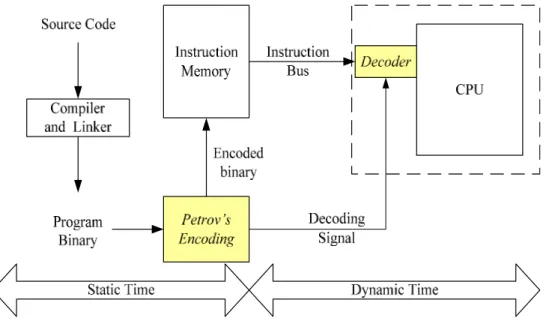
(20) Logic Unit. Index to TT BB1. PC1. τ1τ2τ3 … τn E. BB2. PC2. τ1τ2τ3 … τn E. BB3. PC3. τ1τ2τ3 … τn E . . .. . . .. BBIT. TT. Figure 2-4: Hardware support of BIBITS encoding. 2.2.2. Peter Petrov’s Instruction Bus Encoding Petrov’s bus encoding scheme [5] shown in Figure 2-5 is an application-specific dynamic customization methodology for power minimization in the instruction buses. Fundamentally, it uses application-specific information to identify optimal power encoding. This encoding concentrates the effort on the application hot-spots and encodes the instructions at static time. The encoded instructions reside in the instruction memory, and the processor core receives information about transformation residing in additional table nearby the processor, either when loading the program or when running the software. The processor’s fetch module uses this information to efficiently restore the original bit sequence on each bus line on dynamic time.. -11-.

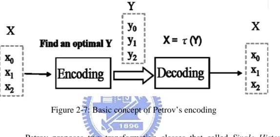
(21) Figure 2-5: Design flow of Petrov’s bus encoding scheme. First, the basic blocks in hot-spots are vertically partitioned into several block words. A block word is an encoding unit and is transformed to a codeword with fewer bit transitions. Consider an arbitrary sequence of bits, a block word X = {…, xn+3, xn+2,…, xn-3,….}. They want to find an alternative sequence of bits, a codeword Y = {…, yn+3, yn+2,…, yn-3,….} and decoding function τ such that the number of bit transitions in Y is minimized and X = τ(...,Y). Given a block word with length k, there are 2k candidate codewords; and the encoder have to select the most suitable one that not only the bit transitions is minimized but also decodable by some decoding function τ.. Figure 2-6 shows an example for a basic block partitioning with block word length equal to 3-buts, and Figure 2-7 illustrates the basic concept of Petrov’s encoding scheme.. -12-.

(22) Figure 2-6: Basic block partitioning example. Figure 2-7: Basic concept of Petrov’s encoding Petrov proposes two transformation classes that called Single History Bit (SHB) transformations and Double History Bits (DHB) transformations separately. The transformation τ has to satisfy either one of the following transformation equations:. For the SHB transformations. x 0 = y 0 ; x i = τ (y i , x i -1 ), ∀1 ≤ i ≤ k And for the DHB transformations. x0 = y0 ; x1 = y1; xi = τ (x i-1 , x i-2 ), ∀2 ≤ i ≤ k. -13-.

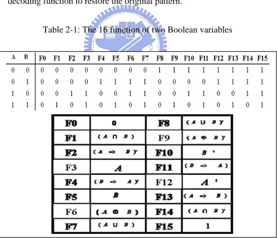
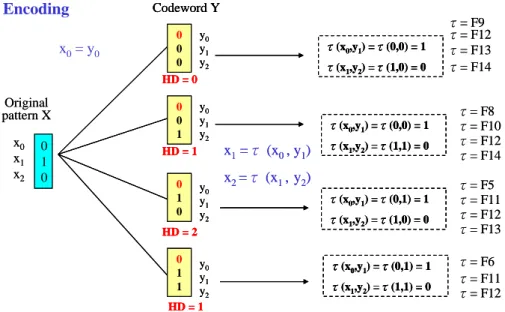
(23) Both classed of transformations are very efficient to compute, since they correspond to simple binary functions with two Boolean variables. The total 2. number of such logic functions is. 22 = 16. for each of the two transformation. types shown in table 2-1. While the decoding architecture will support all 32 distinct functions, only a small subset of transformations identified for a hot-spot would be utilized. Figure 2-7 and Figure 2-8 are 3-bit block word encoding and decoding examples with SHB transformation. In Figure 2-7, Codeword 000 is selected since it can reduce the most bit transitions and also have at least one decoding function to restore the original pattern. Table 2-1: The 16 function of two Boolean variables. -14-.

(24) Encoding. Codeword Y y0 0 y1 0 y2 0 HD = 0. x0 = y0. Original pattern X x0 x1 x2. y0 0 y1 0 y2 1 HD = 1. 0 1 0. 0 1 0. y0 y1 y2. τ(x0,y1) =τ(0,0) = 1 τ(x1,y2) =τ(1,0) = 0. τ(x0,y1) =τ(0,0) = 1. x1 =τ (x0 , y1). τ(x1,y2) =τ(1,1) = 0. x2 =τ (x1 , y2) τ(x0,y1) =τ(0,1) = 1 τ(x1,y2) =τ(1,0) = 0. HD = 2 0 1 1. y0 y1 y2 HD = 1. τ(x0,y1) =τ(0,1) = 1 τ(x1,y2) =τ(1,1) = 0. τ= F9 τ= F12 τ= F13 τ= F14 τ= F8 τ= F10 τ= F12 τ= F14 τ= F5 τ= F11 τ= F12 τ= F13 τ= F6 τ= F11 τ= F12. Figure 2-7: Petrov’s encoding example. Decoding x0 = y0, xi =τ(xi-1, yi ). Codeword Y. y0 0 y1 0 y2 0 τ= F9. x0 = y0 = 0 x1=τ(x0 , y1) = x 0 ' = 1 x2=τ(x1 , y2) = x1 ' = 0. Original pattern X. 0 x0 1 x1 0 x2. Figure 2-8: Petrov’s decoding example The hardware support of this implementation is presented in Figure 2-9. The Basic Block Identification Table (BBIT), as shown in Figure 2-9(a), contains the program counter of the starting instruction together with an index into Transformation Table (TT), as shown in Figure 2-9(b). A TT entry contains the transformation information needed to handle as a single block word for each bus line. The last TT entry for a particular basic block must contain information about how long the last code word is. The End(E) bit field in the TT entry is assert for the entries that correspond to the block word for a given basic block. The CT field. -15-.

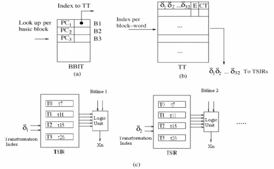
(25) is a counter corresponding to the size of the last bit sequence. The transformation subset identification registers (TSIR), shown in Figure 2-9(c) is proposed as a means of selecting a predetermined subset of transformations. The TSIR contains a set of five-bit registers. The values stored in these registers are used as control signals for selecting any one of the supported 32 Boolean functions, which can be easily implemented in the form of a universal logic unit. The example architecture presented in Figure 2-9(c) supports up to four transformations with four TSIR. The transformation indices selected for a particular program hot-spot are stored into these registers prior to entering the loop. Subsequently, each of the selected transformations is encoded as a short index, in the case of Figure 2-9(c), two bits, which is stored as δi in the TT table to represent the specific transformation. The index is used to select the TSIR register, which in turn produces the actual five bit transformation index.. Figure 2-9: Hardware support of Petrov’s encoding. -16-.

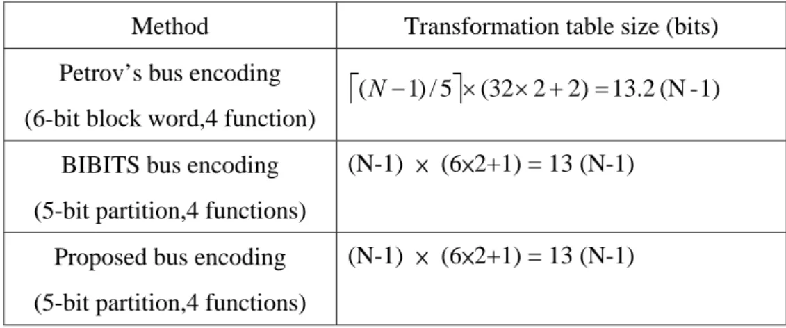
(26) 2.2.3. Summary of previous Researches This section gives a brief summary of previous researches. Both BIBITS and Petrov’s encoding scheme are efficient for programs include frequently executed loops and no encoder hardware overhead requirement.. BIBITS encoding scheme is simlpe that only uses four Boolean functions for encoding and decoding, which are: Identity, Invert, XOR and XNOR, and all of them satisfy the property that one partition can be encoded and decoded with the same Boolean function.. Petrov’s bus encoding scheme is more coplicated than BIBITS that uses unlimited transformation for encoding and fixed number of deocding functions for each hotspot. Thus it has more flexibility for encoding and decoding function selections. However, it need more complicated logic circuit and larger transformation table for decoding.. We assume that there are N instructions in some basic block. What about actual transformation table size use by these schemes when all basic blocks are encoded? Results of these are presented in Table 2-2. We can find that Petrov’s table size is larger than the others.. -17-.

(27) Table 2-2: Comparison with transformation table size Method Petrov’s bus encoding. Transformation table size (bits). ⎡( N − 1) / 5⎤ × (32 × 2 + 2) = 13.2 (N - 1). (6-bit block word,4 function) BIBITS bus encoding. (N-1) × (6×2+1) = 13 (N-1). (5-bit partition,4 functions) Proposed bus encoding. (N-1) × (6×2+1) = 13 (N-1). (5-bit partition,4 functions). We compare of the techniques in Table 2-2. We also list our design here to compare with these methods. The detail description of our design will be discussed in the next chapter.. Table 2-2: Comparison of the instruction bus encoding techniques Techniques. Our BIBITS. Petrov’s design. Less Decoding Function. Flexible. Flexible. Lower. Higher. Higher. Smaller. Larger. Smaller. Lower. Higher. Higher. flexible Decoding Circuit Complexity Transformation Table Size Decoder Energy Overhead Not Energy saving. Good. Better well. -18-.

(28) Chapter 3. Design of Proposed Encoding. The design of our proposed bus encoding scheme to reduce the number of bit transitions on instruction bus is introduced in this chapter. The design flow of applying the proposed methodology is illustrated in Figure 3-1. Our encoding concentrates the effort on the application hot-spots and encodes the instructions at static time. The encoded instructions reside in the program memory, and the processor core receives information about transformation residing in additional table nearby the processor, either when loading the program or when running the software. The processor’s fetch module uses this information to efficiently restore the original bit sequence at dynamic time. We will describe each added component in the following sections.. Source Code Instruction Bus. Instruction Memory. Decoder CPU. Compiler and Linker Encoded binary Proposed Encoding. Program Binary. Decoding Signal. Static Time. Dynamic Time. Figure 3-1: Design flow of our bus encoding. -19-.

(29) 3.1. Our Bus Encoding Scheme Fundamentally, our encoding scheme uses application-specific information to identify optimal power encoding. The encoding scheme is divided as three phase: encoding method algorithm, decoding function selection and hardware mechanism. The part of encoding method algorithm introduces how we encode instructions at static time. Then we introduce our decoding function selection method which can efficiently select a subset of decoding functions for each hotspot. At last we discuss the hardware support and the overhead in terms of power consumption.. First, an instruction is partitioned into several fields with k-bit size (k=1~32), and each field is as an encoding unit. While the bus width is typically 32-bits, for some partition size k, such as 3, 5 and 6 etc, it is impossible to partition an instruction into fields with the same size. We let the remainder bits with fewer switching activities in one partition and not encode them. In this way, all other partitions are in k-bit groups. Figure 3-2 shows an example for instruction partitioning given the partition size equal to 4-bits and 5-bits, respectively. Two bit in gray are not encoded cause they have relative fewer switching activities.. -20-.

(30) 4-bits partition size 1010. 1000. 0010. 0100. 00001. 00100. 0010. 1001. 0111. 1000. 5-bits partition size 1. 0. 1010. 00101. 00101. 1. 11000. Figure 3-2: Instruction partitioning example All partitions in the first instruction of the basic block are not encoded. Then, sequentially encode each partition of the other instructions. Each partition of current instruction is compared with the corresponding partition of previous instruction, and the most suitable codeword with fewest bit transitions is chosen.. Given a bit pattern X ={X0, X1, …, Xk-1}, we want to finding a codeword Y = {Y0,Y1, …,Yk-1} and a decoding function τ such that the Hamming distance between the current pattern and the previous encoded pattern is minimized and X = τ(...,Y). Given a block word with length k, there are 2k candidate codewords; and the encoder have to select the most suitable one that not only the bit transitions is minimized but also decodable by some decoding function τ. The basic concept of our bus encoding is shown in Figure 3-3.. -21-.

(31) Figure 3-3: Basic concept of our encoding When identifying an codeword Y, the mappingτis also identified for the partition to restore the original pattern.. We proposed two transformation classes as follow, and both of them can easily help us to restore the original pattern.. Type 1:. X i = Xi-1 OP Y i. Type 2:. X i = Y i-1 OP Y i. Where X i and X i-1 represent original pattern of current cycle and of previous cycle respectively, Yi and Yi-1 represent encoded pattern of current cycle and of previous cycle respectively, and OP represents the Boolean operation.. The first class of transformations is satisfied if the original pattern can be restored through the operation of previous original pattern and current codeword, while the second one is satisfied if the original pattern can be restored through the operation of previous codeword and current codeword. Both classes of transformations are very efficient to compute, since they correspond to simple. -22-.

(32) Boolean operations two variables. The total number of such logic operations is 2. 22 = 16 for each of the two transformation types. Table 2-1 shows the 16 logic operations of two one-bit Boolean variables.. Figure 3-4 and Figure 3-5 are 5-bit partition encoding and decoding examples. In this example, 01101 is identified as the most suitable codeword because it has fewest bit transitions and also it satisfies one of the transformation equations. In figure 3-5, the codeword 01101 is restored by the transformation function.. Figure 3-4: Encoding example of our encoding scheme. Figure 3-5: Decoding example of our encoding scheme. -23-.

(33) In order to be able to decode the original bit sequence, we need a special hardware support on the processor side which needs to know which transformation is associated to each partition. This information is communicated prior to entering the hot-spot, thus introducing no performance overhead in practice. We store the transformation information of each partition into a transformation table nearby the processor for restoring the original bit sequences. However, the amount of this information determines the area and power consumption of the specialized hardware. Therefore, it has to minimize this amount, while achieving significant reduction of bit transitions. Further more, we also need a decoding function selection method to select the most effective N decoding functions for a hotspot, where N =2i, 0 < i <5. Once the decoding functions have been selected for each hotspot, we can use a short index in the transformation table to identify the decoding function of each partition.. Our decoding function selection method is as follow:. 1. Pseudo encode the hotspot with all possible (32τ) decoding functions. 2. Statistic the frequency of each decoding function that can decode a most suitable codeword. 3. Select N decoding functions with the highest frequency for the hotspot.. -24-.

(34) We model the problem as a maximal cover set problem:. At first, we give a definition : setj = { codewords with minimal bit transitions and decodible by function j, j=0~32}. And we want to select N sets such that Setn 0 U Setn1 U ... U Setn − 1 is maximal. Figure 3-6 shows an example with j=0~2 and N = 2. We can easily observe that Setn1 U Setn 2 is maximal, i.e. Set1 and Set2 have the maximal cover. Therefore, function1 and function2 are selected as decoding functions for the hot spot.. Figure 3-6: Function selection example In next section, we will introduce the hardware support and describe the functionality of each component for our bus encoding scheme.. 3.2. Hardware support The hardware mechanism consists of three main modules: basic-block identification table, transformation table and decoding logic. The block diagram of the proposed method is shown in Figure 3-7. The blocks inside the dotted line are our designed circuits, the decoding-control logic, that contain four elements:. -25-.

(35) instruction fetcher, basic block identification table, transformation table, and decoding logic. This hardware mechanism may be combined with processor core into a single chip.. Figure 3-7: Decoder organization The decoder is responsible for sending instructions to processor from memory. It first fetches instructions from memory and then determines if the fetched instruction is an encoded instruction. If the fetched instruction is an encoded instruction, the original instructions will be gathered from the decoder. The decoder consists of four components: instruction fetcher, basic block identification table, transformation table, and decoding logic. Figure 3-8 shows the organization of each component.. 1. Instruction Fetcher:. -26-.

(36) The instruction fetcher receives the program-counter address request from processor.. 2. Basic Block Identification Table (BBIT):. The basic block Identification table stores the program counter value of the starting instruction and an index that points to the first entry in the transformation table for this basic block. The number of entries in this table corresponds to the number of encoded basic blocks for the particular application loop. 3. Transformation Table (TT):. The transformation table stores transformation data £nn associated with each encoded partition from the instruction memory. A TT entry contains the control bits for selecting the transformation associated with each partition. The hardware structure asserts the end bit field (E) in the TT entry for entries corresponding to the last partition word in a given basic block.. 4. Decoding logic:. The decoding logic receives the control bits τn from TT and indexing TSIR, and selects decoder function to restore each partition of encoded instructions.. -27-.

(37) Figure 3-8: Organization of each decoding component. -28-.

(38) Chapter 4. Simulation and Analysis. In this chapter, we first introduce a set of six benchmarks we have used for our experimental study. Then we introduce the simulation methods in this thesis, including the toolsets, simulation flow, simulation parameters and evaluating factors.. 4.1. Experimental Benchmarks To evaluate the efficiency of encoding in bus transition reduction, we perform experiments for the following six benchmarks. These benchmarks contain various DSP and numerical-computation kernels that represent code frequently encountered in many embedded system products. Table 4-1 gives a summary of the application benchmarks we used. and Table 4-2 shows the size and basic block number of each benchmark program. Table 4-1: Benchmarks Function Name. Description. Jacobi. Extrapolated Jacobi-iterative method on a 128 × 128 entry grid.. FFT. Fast Fourier transform with block size of 256 samples. Lower/upper triangular matrix decomposition algorithm on a. LU matrix of size 128 × 128. Mmul. A matrix multiplication on a matrix of size 100 × 100. SOR. Successive over-relaxation on a matrix with size 128 × 128.. Tri. Tri-diagonal system solver on a matrix of size 128 × 128. -29-.

(39) Table 4-2: Benchmark program size and numbers of each basic block Program. 4.2. Program size (Bytes). Number of Basic Block. Mmul. 321. 14. Sor. 1600. 18. Ej. 1350. 25. FFT. 1241. 82. Tri. 1300. 13. LU. 3420. 38. Experimental Methods In this Section, we introduce the experimental toolset we used for the simulation. The basic tool for this experiment is the release 6.02 of MIPS® SDE Lite, a free subset of the MIPS Software Toolkit [7] which is used to built MIPS environment, and therefore we can get the execution trace of each application benchmark for the simulation of bus encoding. Furthermore, we additionally wrote a simulation tool to do basic block selection, decoding function selection, and bus encoding schemes. At last, we list the experimental flow, the experiments we planned to do, and simulation parameters we referred.. 4.3. Experimental Toolset Our experimental environment is divided into three sub-environments:. Code generation phase The purpose of this phase is to compile the executable binary codes for the. -30-.

(40) benchmark programs. We adopt the release 6.02 of the MIPS SDE tool chain : a component of the MIPS Software Toolkit to build the MIPS ELF (Executable and Linkable Format) image format for each benchmark program Transformation table building phase This phase includes a transformation table builder and a code-rebuilder. The transformation table builder scans the program execution trace running under the GNU MIPS CPU Simulator and builds the transformation table which stored the transformation information for decoding. The code-rebuilder rebuilds the program with the transformation table provided from the transformation table builder Result calculation phase The final sub-environment includes the modified simulator and the bit transition calculator and energy consumption estimator to show the experiment result.. To construct the experimental environment, we have adopted and developed the complete experimental toolset consisting of individual tools that accomplish specific tasks respectively. Table 4-3 lists all tools composing the experimental toolset.. -31-.

(41) Table 4-3: Experimental toolset descriptions Tool Name. Description SDE’s version of the Free Software Foundation’s. sde-gcc ANSI-compatible GNU C Compiler compiling C source code. The GNU MIPS CPU simulator executes the MIPS ELF image sde-run files. It could generate the trace of the benchmark programs. The Basic Block Selector that builds the recovery codebook with BB-select codebook building rules by scanning the program execution trace. The code-rebuilder rebuilds the program with the transformation code-rebuild table provided from the transformation table builder. The modified GNU MIPS CPU simulator to execute the encoded modsde-run. programs and calculate the bit transitions and estimate energy consumption on instruction bus.. 4.3.1. Experimental Flow The experimental flow, the experimental toolset and intermediate files, such as object files, MIPS ELF files, etc., are shown in Figure 4-1. By a horizontal dotted line, this figure is divided into three sub-figures representing the three experimental. sub-environments. representing. the. three. experimental. sub-environments.. The complete experimental flow is described as follows:. 1. The MIPS C compiler (sde-gcc) compiles the source files (.c) of the. -32-.

(42) benchmark programs into its corresponding object files (.o).. 2. The MIPS C linker (sde-ld) links the object files necessary for building MIPS ELF files of the components in the benchmark suite.. 3. The GNU MIPS CPU Simulator (sde-run) traces the ELF files with input data and then output the execution instructions and the corresponding program counters (PC value).. 4. The Basic Block Selector (BB-sel) scans execution trace and produces the BBIT and TT that contain selected basic block and encoding information.. -33-.

(43) Figure 4-1: Experimental flow by using our experimental toolset 5. According to the TT files, the code-rebuilder build the MIPS machine code files.. 6. The modified GNU MIPS CPU Simulator (modsde-run) executes the coded programs with transformation tables and input data. It also calculates the bit transitions for executing these programs, and estimate the energy consumption on instruction bus.. -34-.

(44) 4.3.2. Designing Experiments In our simulation, we evaluate the bit transitions and the energy consumption of these following conditions:. 1. Base system architecture without any bus encoding:. This is the simply architecture with only the processor and instruction memory.. 2. BIBITS:. This is the power reduction technique we mentioned in the Chapter 2. We implement this architecture to compare the results with ours.. 3. Petrov’s bus encoding scheme: This is also the power reduction technique we mentioned in the Chapter 2. We implement this architecture to compare the results with ours. Our bus encoding scheme. This is our design that we execute the coded program with the recovery dictionary. We will evaluate the bit transitions of all these schemes with different transformation table sizes.. 4.4. Simulation Results and Analyses In this Chapter, we present the experimental results obtained from evaluating energy consumed by the benchmark programs. We first evaluate the bit transitions. -35-.

(45) reduction and energy saving for our encoding in different number of decoding functions and partition sizes. Then we evaluate the bit transtions reduction and energy saving by various techniques. Then we evaluate the bit transitions reduction of BIBITS, Petrov’s bus encoding scheme and ours in different transformation table sizes. Notice that the results of bit transition are all normalized to those of the base system.. 4.4.1. Hardware Overhead Analysis To pevaluate the power overhead of decoder, we have utilized the Cacti tool [8] to obtain the energy consumption associated with the TT and the BBIT tables. A 0.18-μm process technology with 1.7V voltage level has been used. we assume the bus line capacitance is 30 pF. We have found thay an access to the TT (1.5 Kbyte) consumes approximately 39 pJ of energy while an access to the BBIT (0.2KByte) consumes 82.3 pJ. The decoding logic consumes is negligibly small and amounts 0.038 pJ [6]. According to the switching power equation introduced in Section 2.1, a single bit transition consumes 57.8 pJ. We not only evaluate the bit transition reductions of these bus encoding techniques, but also estimate the energy saving that also take overhead into consideration.. 4.4.2. Bit Transition Reduction and Energy Saving of Our Encoding We measure our approach’s effectiveness by observing the energy saving. We. -36-.

(46) ran simulation using a typical embedded processor as the baseline system architecture with a set of benchmarks.. Figure 4-2 and Figure 4-3 shows the bit transitions reduction ratio and energy saving for our encoding with different number of decoding functions and partition sizes respectively. All basic block in program are encoded, and each basic block can have its own small set of decoding function candidates. We find that our encoding can save most energy when the number of decoding function candidates is four and the partition size is five bits.. average. Bit transition reduction. 80.00% 70.00% 60.00% 50.00% 40.00% 30.00% 20.00% 10.00%. Ou. r_ 2 Ou τ _ r_ 2 4 Ou τ _ r_ 2 Ou 8τ r_ _2 32 Ou τ _ r_ 2 2 Ou τ _ r_ 3 4 Ou τ _ r_ 3 Ou 8τ r_ _3 32 Ou τ _ r_ 3 2 Ou τ _ r_ 4 4 Ou τ _ r_ 4 Ou 8τ r_ _4 32 Ou τ _ r_ 4 2 Ou τ _ r_ 5 4 Ou τ _ r_ 5 Ou 8τ r_ _5 32 Ou τ _ r_ 5 2 Ou τ _ r_ 6 4 Ou τ _ r_ 6 Ou 8τ r_ _6 32 τ _6. 0.00%. Our encoding. Figure 4-2: Bit transition reduction ratio of our encoding with different number of decoding functions and partition sizes. -37-.

(47) average 60.00%. Energy saving. 50.00% 40.00% 30.00% 20.00% 10.00%. Ou. r_ 2 Ou τ r _ _2 Ou 4 τ r _2 O u _8 τ r _ _2 3 O u 2τ r _ _2 Ou 2 τ r _ _3 4 Ou τ r _ _3 Ou 8 τ r _ _3 3 O u 2τ r _ _3 2 Ou τ r _ _4 Ou 4 τ r _ _4 Ou 8τ r _ _4 3 O u 2τ r _ _4 Ou 2 τ r _ _5 4 Ou τ r _ _5 Ou 8 τ r _ _5 3 O u 2τ r _ _5 Ou 2 τ r _ _6 Ou 4 τ r _ _6 Ou 8τ r _ _6 32 τ _6. 0.00%. Our encoding. Figure 4-3: Energy saving of our encoding with different number of decoding functions and partition size. 4.4.3. Bit Transition Reduction of Different Techniques Figure 4-4 and Figure 4-5 display the bit transition reduction and energy saving by applying different techniques in six different benchmark programs respectively. There are four techniques applied in the figures: BIBITS, Petrov’s bus encoding scheme, our proposed bus encoding scheme, and our bus encoding scheme with optimal decoding function selection. All basic block in program are encoded and each basic block can have his own small set of decoding function candidates.. -38-.

(48) Petrov's_4T_6. BIBITS_4τ_5. Our_4τ_5. Our_4τ(opt)_5. 80.00%. Bit transition reduction. 70.00% 60.00% 50.00% 40.00% 30.00% 20.00% 10.00% 0.00% tri. jacobi. lu. sor. fft. mmul. average. Figure 4-4: Bit transition reduction of different techniques Petrov's_4T_6. BIBITS_4τ_5. Our_4τ_5. Our_4τ(opt)_5. 80.00% 70.00%. Energy saving. 60.00% 50.00% 40.00% 30.00% 20.00% 10.00% 0.00% tri. jacobi. lu. sor. fft. mmul. average. Figure 4-5: Energy saving of different techniques Experimental results indicate that our proposed encoding scheme can save energy range around 49% to 68% except for the fft program. The overall average energy saving is 52% over original data and 16% more than Petrov's bus encoding scheme only and 6% more than BIBITS encoding scheme only.. -39-.

(49) 4.4.4. Bit. Transition. Reduction. of. Techniques. with. Different. Transformation Table Sizes In this section we will evaluate the bit transition effects for all these encoding scheme with different transformation table sizes.. Figure 4-6 shows the bit transition reduction of mmul program with different transformation table sizes. Our scheme has higher bit transition reduction than the others. These following figures are experiment result of each benchmark program.. BIBITS. Our _ 4τ_5. petrov_ 4τ_6. 70.00%. Bit transition reduction. 60.00% 50.00% 40.00% 30.00% 20.00% 10.00% 0.00% 0. 0.5. 1. 1.5. 2. TT size (KB). Figure 4-6: mmul - Bit transition reduction with different transformation table sizes BIBITS. Our _ 4τ_5. petrov_ 4τ_6. 80.00% Bit transition reduction. 70.00% 60.00% 50.00% 40.00% 30.00% 20.00% 10.00% 0.00% 0. 1. 2. 3. 4. TT size (KB). Figure 4-7: sor - bit transition reduction with different transformation table sizes. -40-.

(50) BIBITS. Our _ 4τ_5. petrov_ 4τ_6. 70.00% Bit ttransition reduction. 60.00% 50.00% 40.00% 30.00% 20.00% 10.00% 0.00% 0. 0.5. 1. 1.5. 2. 2.5. 3. 3.5. 4. 4.5. TT size (KB). Figure 4-8: jacobi - bit transition reduction with different transformation table sizes BIBITS. Our _ 4τ_5. petrov_ 4τ_6. 50.00%. Bit transition reduction. 45.00% 40.00% 35.00% 30.00% 25.00% 20.00% 15.00% 10.00% 5.00% 0.00% 0. 0.5. 1. 1.5. 2. 2.5. TT size (KB). Figure 4-9: fft - bit transition reduction with different transformation table sizes BIBITS. Our_4τ_5. petrov_ 4τ_6. 70.00%. Bit transition reduction. 60.00% 50.00% 40.00% 30.00% 20.00% 10.00% 0.00% 0. 0.5. 1. 1.5. 2. 2.5. 3. 3.5. 4. 4.5. TT size (KB). Figure 4-10: tri - bit transition reduction with different transformation table sizes. -41-.

(51) BIBITS. Our _ 4τ_5. petrov_ 4τ_6. 70.00%. Bit transition reduction. 60.00% 50.00% 40.00% 30.00% 20.00% 10.00% 0.00% 0. 0.5. 1. 1.5. 2. 2.5. 3. 3.5. 4. 4.5. TT size (KB). Figure 4-11: lu - bit transition reduction with different transformation table sizes We observe that our method has higher bit transition reduction than the other schemes. The Figure 4-12 displays the average bit transition reductions for full benchmarks with different transformation table sizes.. p etro v _ 4 τ_ 6. BIBITS_ 4 τ_ 5. Ou r _ 4 τ_ 5. Bit transition reduction. 70.00% 60.00% 50.00% 40.00% 30.00% 20.00% 10.00% 0.00% 0. 0.5. 1. 1.5. 2. 2.5. 3. 3.5. 4. 4.5. TT_ size(KB). Figure 4-12: Average bit transition reduction for full benchmarks with different transformation table sizes. -42-.

(52) Chapter 5. Conclusion and Future Works. In this thesis, we proposed a bus encoding scheme to reduce power consumption on instruction bus. The key idea of our method is to apply a transformation table which stores frequently execution basic block transformation data to make use of repetitions of basic blocks at program execution time for reducing bit transitions on instruction bus. The simulation results show that the overall average energy saving is 52% over original data and 16% more than Petrov's bus encoding scheme only and 6% more than BIBITS encoding scheme only. The suitable size of transformation table varies with different application benchmarks. Our transformation table size is equal to BIBITS and smaller than Petrov’s encoding. Therefore, the extra hardware overhead of our proposed is lower than Petrov’s bus encoding scheme. There are still several researches issues for better energy saving. For example, it the first instruction in a basic block can also be encoded, the bit transitions can be further reduced. A possible approach is using off-line profile and analyzing control flow graph to identify the instruction encountered before the first instruction in a basic block. Furthermore, it is possible to find some compiler techniques such as instruction reordering to combine with bus encoding to further reduce the bit transitions.. -43-.

(53) Reference [1] A.P. Chandrakasan, S. Sheng, and R.W. Brodersen, “Low-Power CMOS Digital Design,” IEEE Journal of Solid-State Circuits, Vol. 27, No. 4, pp. 473-483, Apr.1992. [2] A. Chandrakasan, R. Brodersen, “Minimizing Power Consumption in Digital CMOS Circuits,” Proceedings of the IEEE, Vol. 83, No. 4, pp. 498-523, April 1995. [3] K. Choi, W. Lee, R. Soma, and M. Pedram, “Dynamic Voltage and Frequency Scaling Under a Precise Energy Model Considering Variable and Fixed Components of the System Power Dissipation,” Proc. of International Conference on Computer Aided Design (ICCAD), Nov. 2004. [4] Kiran Puttaswamy et al. “System Level Power-Performance Trade-offs in Embedded Systems Using Voltage and Frequency Scaling of Off-chip Buses and Memory,” ISSS’02, Pages: 225 – 230 Oct.2002. [5] Chin-Tzung Cheng, Wei-Hau Chiao, Jean Jyh-Jiun Shann, Chung-Ping Chung, and Wen-Feng Chen, “Low-power BIBITS Encoding with Register Relabeling for Instruction Bus,” 2005 IEEE VLSI-TSA International Symposium on VLSI Design, Automation, and Test (VLSI-TSA-DAT’05) [6] P.petrov and A.Orailoglu, “Low-Power Instruction Bus Encoding for Embedded Processors,” IEEE Transactions on VLSI,VOL. 12, NO. 8, Aug. 2004. [7] MIPS Technologies, Inc., “MIPS SDE 6.02 Programmers’ Guide,” Jan 2004 [8] P.Shivakumar and N.Jouppi, “CACTI 3.0 : An integrated cache timing, power and area model,” Western Research Lab., 2001.. -44-.

(54)