崩積地層工址特性評估與大地工程問題---子計畫：崩積地層之調查與監測---電學方法(III)

行政院國家科學委員會補助專題研究計畫

■ 成 果 報 告

□期中進度報告

崩積地層之調查與監測-電學方法

Subsurface Investigations and Monitoring in Colluvium - Electrical

Methods

計畫類別：□ 個別型計畫

■

整合型計畫

計畫編號：NSC 95－2221－E－009－200－

執行期間： 94 年 8 月 1 日至 97 年 7 月 31 日

計畫主持人：

林志平 國立交通大學土木工程系

共同主持人：

計畫參與人員：

湯士弘 國立交通大學土木工程系

鍾志忠 國立交通大學土木工程系

姚奕全 國立交通大學土木工程系

吳瑋晉 國立交通大學土木工程系

林哲毅 國立交通大學土木工程系

成果報告類型(依經費核定清單規定繳交)：□精簡報告

■

完整報告

本成果報告包括以下應繳交之附件：

□赴國外出差或研習心得報告一份

□赴大陸地區出差或研習心得報告一份

■

出席國際學術會議心得報告及發表之論文各一份

□國際合作研究計畫國外研究報告書一份

處理方式：除產學合作研究計畫、提升產業技術及人才培育研究計畫、

列管計畫及下列情形者外，得立即公開查詢

□涉及專利或其他智慧財產權，□一年□二年後可公開查詢

執行單位：

國立交通大學土木系

中 華 民 國 97 年 10 月 30 日

1

行政院國家科學委員會專題研究計畫成果報告

崩積地層之調查與監測-電學方法

Subsurface Investigations and Monitoring in Colluvium - Electrical

Methods

計畫編號：

NSC 95－2221－E－009－200－

執行期限：94 年 8 月 1 日至 97 年 7 月 31 日

主持人：林志平 國立交通大學土木工程系

一、中文摘要 崩積地層之鑽探調查非常困難，而其穩 定性又常由降雨入滲與地下水位所控制，利 用非侵入式的地電阻法輔助工址調查及以 電學性質監測地層之含水特性應該是值得 發展的方向。崩積地層及殘餘土內之含水 量、飽和度、與地水位，影響崩積層邊坡之 穩定性甚巨，而地層含水特性與電學性質 （包括電阻率與介電度）具有密切的關連 性，本計畫旨在發展以電學性質調查地層分 佈及監測崩積地層之含水量、土壤吸力、地 水位之技術。本計畫所採用之量測方法包括 時域反射（TDR）量測技術與地電阻影像剖 面技術（ERT），TDR 是以導波器探測頭量 測土壤之電阻率與介電頻譜，而 ERT 則可 以非侵入的方式量測電阻率之二維分佈。 ERT 雖可以非破壞性的方法進行大範圍的 2-D 探測，但單一電阻率量測值受到許多物 理性質所影響（如含水量、土壤種類及地下 水特性等），TDR 介電頻譜較能直接反應 土壤含水量與土壤種類。因此本研究首先建 立並改良 TDR 與 ERT 量測系統，建立崩積 土之電學性質資料庫，再推導崩積土層含水 特性與電學性質間之關係，並討論判讀 ERT 影像剖面資料之原則，最終目的希望能發展 適合崩積地層之 TDR 多功能邊坡監測系統 包括降雨量、含水量、土壤吸力、地水位與 變形，及可提供在空間上與時間上連續資料 的自動化 ERT 監測系統。 本研究計畫為三年期整合型研究計畫 『崩積地層工址特性評估與大地工程問題』 其中子計畫之一，本報告簡述本計畫之執行 成果。 關鍵詞：崩積層、時域反射法、地電阻影像 探測 Abstract

Drilling in colluvium, and especially in talus, is difficult, relatively expensive, and often does not provide the geotechnical engineer with a complete profile of the deposit. Intense rainfall is cited as the most common triggering mechanism for landslides involving colluvium. Hence, electrical geophysical methods hold great promise to supplement drilling data and determine hydrogeological conditions in colluvium. The main objectives of this study is to develop electrical techniques for site investigation and monitoring soil water content, matrix suction, and groundwater level in colluvium. Methods utilized include time domain reflectometry and electrical resistivity tomography. ERT is a non-destructive method that can estimate 2-D distribution of ground resistivity. However, interpretation of the resistivity alone for soil properties is difficult because it is sensitive to many factors, such as water content, soil types and ground water characteristics. TDR uses a waveguide probe to measure soil dielectric spectrum and resistivity. The dielectric permittivity provides extra information for estimating soil water content and soil types. This study will first establish and improve the TDR and ERT measuring methodology. A database will be constructed for electrical properties of colluvial materials. The relationship between soil water retention characteristic and electrical properties will then be established. Guidelines for interpreting ERT resistivity tomograms will be subsequently illustrated. The final goal is to develop a multi-function TDR monitoring system for colluvial slopes including rainfall, water content, matrix suction, groundwater level, and slope deformation. An ERT monitoring system will also be developed to obtain information

2 which is continuous in both space and time. This report briefly describes the study result of this prject.

Keywords: Colluvium, Time Domain Reflectometry, Electrical Resistivity Tomography 二、計畫緣由與目的

崩積地層可能是最為普遍的地表覆蓋

層，Costa and Baker (1981) 估計在潮濕氣候

地區超過 95%的地表面為崩積層所覆蓋。台 灣由於地震頻繁，整體地質環境脆弱，加上 氣候潮濕、地形陡峻、河川溪流侵蝕旺盛， 山區崩坍的岩石及土壤物質容易因滾落、滑 動、崩塌等經過位移作用而在崖錐或邊坡下 方原有的地層之上堆積，形成「崩積層」或 「崩積土」，覆蓋於原出露之地盤上。崩積 層邊坡常具有高度活動性，因此，當工程或 土地利用位於或通過崩積層組成之邊坡，常 引致重大災害以及可觀之經濟損失，如新 店、外雙溪地區數處山坡地上之大型社區、 中橫公路梨山地區、..等等邊坡問題，都屬 於崩塌地之不穩定邊坡問題。 崩積地層因為受到原有邊坡材料、破壞 型態、形成年代等的影響，具高度的不均質 性、不易調查性、及實驗結果代表性不足等 現象，因此，無論力學或水力特性均不易掌 握。雖然國內外已有許多相關研究報告，但 是仍有不少有關崩積層的問題仍有其進一 步研討，譬如：地形地相與過去崩滑、位移、 堆積歷史與崩積層型態與特性的因果關係 與研判，地下水與逕流入滲的影響與分析， 風化與侵蝕的角色與影響，含水量/飽和度 的變化與穩定性之關連，崩積層材料具代表 性之力學行為與力學性質及力學模式、崩積 層破壞機制及模式、崩積層邊坡之復發性及 漸進性破壞的分析方法、推估材料參數的合 宜手段、合理考量材料性質高度不確定性的 途徑、和最佳的工址調查計畫等。上述待釐 清的問題非單一計畫所能完成，本研究團隊 因 此 擬 針 對 這 些 問 題 組 成 整 合 性 研 究 計 畫，推動不同的子計畫，分頭進行同時相互 合作，期能在崩積層之調查、試驗、模擬、 分析等問題上多方面加以研討，本計畫旨在 發展以電學性質調查崩積地層分佈及監測 崩積地層含水量、毛細張力、地水位之技 術。 崩積地層之鑽探調查非常困難，而其穩 定性又常由降雨入滲與地下水位所控制，利 用非侵入式的地電阻法輔助工址調查及以 電學性質監測地層之含水特性應該是值得 發展的方向。崩積地層及殘餘土內之含水 量、飽和度、與地水位，影響崩積層邊坡之 穩定性甚巨，而地層含水特性與電學性質 （包括電阻率與介電度）具有密切的關連 性，本計畫旨在發展以電學性質調查崩積地 層分佈及監測崩積地層之含水量、土壤張 力、地水位之技術。本計畫所採用之量測方 法 包 括 時 域 反 射 （ Time Domain Reflectometry, TDR）量測技術與地電阻影 像 剖 面 技 術 （ Electrical Resistivity Tomography，ERT），TDR 是以導波器探 測頭量測土壤之電阻率與介電頻譜，而 ERT 則可以非侵入的方式量測電阻率之二維分 佈。ERT 雖可以非破壞性的方法進行大範圍 的 2-D 探測，但單一電阻率量測值受到許多 物理性質所影響（如含水量、土壤種類及地 下水特性等），TDR 介電頻譜較能直接反 應土壤含水量與土壤種類。因此本研究首先 建立並改良 TDR 與 ERT 量測系統，建立崩 積土之電學性質資料庫，再推導崩積土層含 水特性與電學性質間之關係，並討論判讀 ERT 影像剖面資料之原則，最終目的希望能 發展適合崩積地層之 TDR 多功能邊坡監測 系統包括降雨量、含水量、土壤吸力、地水 位與變形，及可提供在空間上與時間上連續 資料的自動化 ERT 監測系統。 三、結果與討論 3.1 TDR 量測方法之建立與改良 本研究擬發展適用於崩積層邊坡監測 之含水量、導電度、地層種類、毛細張力及 地下水位等 TDR 量測技術。圖 1a 為 TDR 量測系統的示意圖，它包含階躍脈衝電壓產 生器、訊號採樣器與示波器，脈衝產生器產 生電壓脈衝傳至同軸纜線，訊號採樣器擷取 並透過示波器顯示由同軸纜線傳回之反射 訊號。感測導波器為同軸纜線之延伸使得電 磁波傳進所要量測之材料或環境中。 3.1.1 TDR 全波形模擬 為能夠進一步改良 TDR 之各種量測方 法，特別是在邊坡監測實務上需要不同延長 纜線長度的影響，本研究建構考慮各項因子

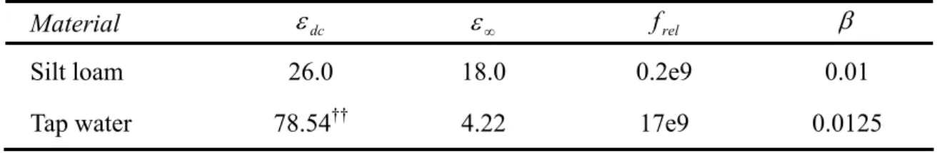
3 的完整 TDR 波傳模型，以作為資料分析及 方法研擬的工具。TDR 傳輸線之波傳控制 方程式可以圖 1b 之電路模型推導得到，其 中 之 單 位 長 度 電 路 參 數 （ conductance g, capacitace c, inductance l, and resistance r）為 介質電學性質與傳輸線幾何的參數，波動控 制 方 程 式 通 解 中 的 主 要 參 數 為 傳 遞 常 數 （ propagation constant γ ） 與 特 徵 阻 抗 （characteristic impedance Zc) ，傳遞常數控 制波傳的速度與衰減，特徵阻抗控制阻抗不 連續面的反射量，在頻率域（f），傳遞常 數與特徵阻抗經推導為 A c f j r * 2π ε * γ = (1a) A Z Z r p c * * ε = (1b) f Z j A R p α η ⎟ ⎟ ⎠ ⎞ ⎜ ⎜ ⎝ ⎛ − + = 0 ) 1 ( 1 (1c) 其中 c 是光速, εr* = εr – jσ/(2πfε0) 是

complex dielectric permittivity（包含介電度 dielectric permittivity εr 及導電度 electrical

conductivity σ之性質，其中ε0 是真空的介電 度）, Zp 是幾何特徵阻抗(真空的特徵阻抗), A 是考慮纜線電阻之修正因子， j 是 −1， 0 η = μ0 /ε0 ≈120π ( μ0 為真空的磁導 率)，α_R (sec-0.5) 是電阻衰減因子（為纜線 的特性）。TDR 量測系統之傳輸線至少包 括延長線段及感應段，不同段之傳遞常數與 特徵阻抗不同，可以多段模式模擬（如圖 2a），每一段可以參數化為傳輸線幾何特性 （Zp）介質電學性質（εr*）、傳輸線電阻衰 減因子（α_R）及段落長度（L），一旦各段 落的這四個參數得知，即可完整模擬 TDR 訊號。波傳的模擬首先先將不同段落的整體 效應以 TDR 起始端的輸入阻抗（input impedance Zin）表示，起始端的輸入阻抗可 由末端阻抗（ZL）及各段落之特徵阻抗以下 式之遞回方式求得：

(

)

(

)

(

)

(

)

( )

( )

11 1 1 , 1 1 1 , 1 1 , 1 1 1 1 , 1 1 1 , 1 1 , 2 , , , 1 tanh ) ( tanh ) ( ) 0 ( tanh ) ( tanh ) ( ) ( tanh tanh ) ( ) ( l z Z Z l Z z Z Z Z l z Z Z l Z z Z Z z Z l Z Z l Z Z Z z Z Z z Z in c c in c in n n n in n c n n n c n in n c n in n n L n c n n n c L n c n in L n in γ γ γ γ γ γ + + = + + = + + = = − − − − − − − − − − − M (2) 其中下標i 代表各段落。一般之 TDR 量測 系統邊界條件為(ZL = ∞). TDR 波形在頻 率域之反應可由輸入阻抗與起始端之邊界 條件推導得到：

( )

_{( )}

( )

S S S in in _{V HV} Z Z Z V = + = 0 0 0 (3) 其中V(0) 是 TDR 波形的富立葉轉換，Vs 是 TDR 輸入方波的富立葉轉換，Zs是源頭阻 抗（source impedance），通常 TDR 儀器之 Zs = 50 Ω， TDR 波形(vt)之模擬可由 V(0) 之富立葉反轉換得到，典型之 TDR 波形如 圖 2c所示。TDR 全波形之模擬與應用詳已 發表之論文Lin and Tang (2007)（附錄 A）.

圖 1 (a) TDR 量測系統 (b) 傳輸線微小元素 之電路模型.

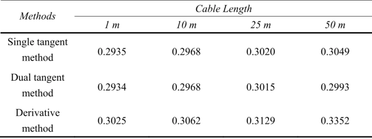
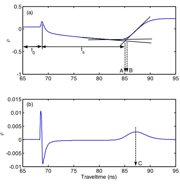
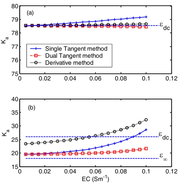
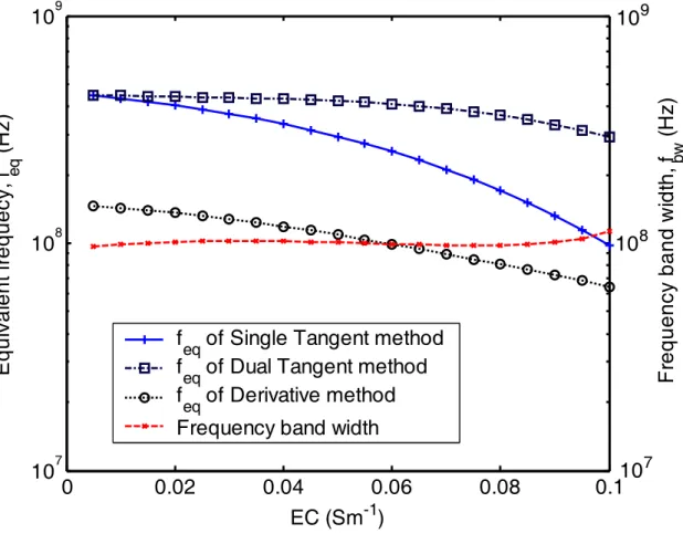
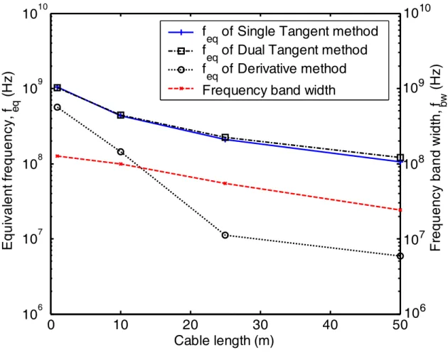
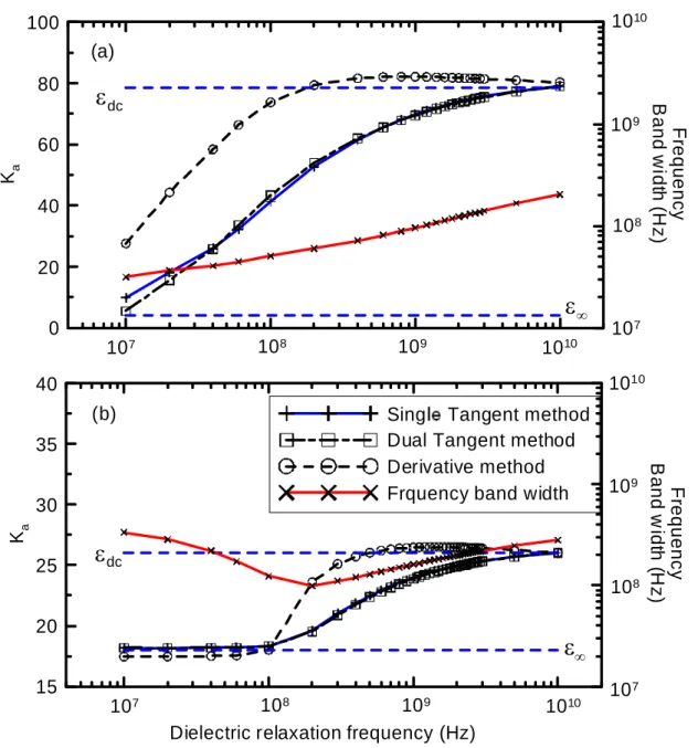
4 圖 2. (a) TDR 量測系統之傳輸線經點模型(b) 直流電電路模型(c)典型 TDR 波形 3.1.2 TDR 含水量量測 材 料 之 基 本 電 學 性 質 包 括 介 電 度 （ Dielectric Permittivity, εr） 與 導 電 度 （Conductivity, σ為電阻率 resistivity 的倒 數）。其中，介電度為頻率之函數，在不同 頻率之電場下，材料有如動態反應譜呈現不 同之介電度。在頻率域，介電度可以表示為 複數，實部（εr'）表示外部電場能量在材料 中之儲存，虛部（εr"）表示阻尼效應之能量 消散。波動方程式在頻率域之解析中，介電 度與導電度兩項材料性質可合併為等值介 電度（εr*）如下式所示 ⎟⎟ ⎠ ⎞ ⎜⎜ ⎝ ⎛ + − = − = 0 2 " ' ' * ε π σ ε ε ε ε ε f j j dc r r ii r r r （4） 其中ε0為真空之介電常數，電磁波在傳輸纜 線中之傳遞常數可寫為 β α ε π γ j c f j r = + = 2 * （5） 其中α 與 β 分別為傳遞係數之實部與虛 部，實部α 反應電磁波之衰減，虛部β 為空 間頻率，時間頻率（2πf）除以空間頻率（β） 可得波傳之相位速度（Phase velocity） ⎟ ⎟ ⎟ ⎠ ⎞ ⎜ ⎜ ⎜ ⎝ ⎛ ⎟ ⎟ ⎠ ⎞ ⎜ ⎜ ⎝ ⎛ + + = = 2 ) ( ' ) ( 1 1 2 ) ( ' 2 ) ( f f f c f f v r ii r r ε ε ε β π (6) 由（6）式可知，因為材料介電性質隨頻率 而異，電磁波之波速也成為頻率的函數，此 種頻散現象(Dispersion) 使得方波於電纜中 傳輸後之波形趨於圓滑，上升斜率趨緩。如 圖 2c 所示，其 TDR 反射訊號之上升時間 （rise time）較原入射方波上升時間長，且 波形較為圓滑。 Topp et al. (1980)以 TDR 在時間域的視 速度(apparent velocity，如圖 2a中的t0所示) 定 義 了 視 介 電 常 數 Ka(apparent dielectric constant)，va與 Ka的關係為(6)式之簡化： a a K c v = (7) 其中視速度通常利用切線分析法決定電磁 波在感測器中的來回走時t0： 0 / 2L t v_a = (8) 因此，視介電常數可利用下式決定： 2 0 2 ⎟⎠ ⎞ ⎜ ⎝ ⎛ = L ct K_a (9) 土壤之介電度與含水量具有高度相關性， Topp et al. (1980)提出Ka與土壤含水量的經 驗公式，獲得良好的含水量量測結果並廣被 引用，但有一些土壤需要經過個別標定方能 得到合理的結果。事實上，視介電度不是一 個真實的物理量，其值受到走時分析方法、 介電度頻散現象、導電度、延長線長度及感 測器末端邊界條件所影響。本研究以 TDR 全波形模擬進行參數研究，廣泛充分探討上 述影響土壤含水量的因子，其中走時分析的 方法包括雙切線法、單切線法及反曲點法， 主要結論如下： „ Ka 的 等 效 頻 率 視 材 料 介 電 頻 散 的 relaxation 頻率，目前並無有效的方法

5 可以決定 Ka的等效頻率。 „ TDR 頻寬範圍內的頻散線現象主要來 自於固相與液相的交互作用，頻散現象 因土壤種類而異，其對於導電度與纜線 長度如何影響Ka扮演關鍵的角色。 „ 如果土壤介電度之頻散現象不明顯，則 Ka不受導電度的影響，且纜線長度的影 響可透過空氣與水之探頭時間點與探 頭長度的標定修正。 „ 若土壤介電度在 TDR 頻寬內展現明顯 的頻散現象，則所量測到之Ka 將受到 導電度的影響及纜線長度的影響。 „ 感測器末端斷路確實會有 fringing 效 應，末端短路可以避免此一問題，末端 短路之感測器可以 TDR 貫入是感測器

（Lin et al. 2006a, 2006b）的形式實現。

„ 雙 切 線 法 所 得 到 Ka 之 等 效 頻 率 最 高，且較導電度與纜線長度之影響較輕 微，但雙切線法的自動化較困難。 „ 單切線法除了受導電度的影響較大之 外，其餘結果與雙切線法類似，但單切 線法不適用於末端短路之感測器。 „ 反曲點法之等效頻率最低，且對於導電 度與纜線長度的影響較敏感，且當導電 度很高或纜線長度很常時會出現不合 理的結果（Ka 高於各頻率之介電度） 上述研究成果對於 TDR 土壤含水量量測的 意義詳已發表之期刊論文（Chung and Lin 2008）（附錄 B）。

現有的 TDR 傳感器不太適合於崩積層 邊坡之監測，在感測器之改良研究方面，建 議利用 TDR 貫入式感測器（Lin et al. 2006a,

2006b）作為崩積地層監測的感測器形式， 並提出末端短路的感測器設計，以降低走時 分 析 受 導 電 度 之 影 響 及 末 端 的 fringing effect，提高後續資料解析的正確性。可量 測土壤含水量剖面及 wetting front 亦是未來 持續努力的目標。 3.1.3 TDR 介電頻譜分析 雖然利用 TDR 視介電度量測土壤含水 量已是眾多電學方法較佳的，但視介電度因 為缺乏明確的物理意義，可能受到土壤種 類、導電度及纜線長度影響，因此本研究將 持續進行 TDR 的介電頻譜分析。 等值介電頻譜（εr*(f)）可經由量測訊號 之系統分析求得，將反射訊號之富立葉轉換 （Y(f)）除以脈衝產生器之入射訊號（X(f)） 可得 TDR 量測系統之系統函數（System function, H）之量測值，此量測值必須等於 量測系統之理論系統函數，如下式表示

(

)

( )

_{( )}

f X f Y f H εr*, = （10） 理論系統函數為纜線阻抗、纜線傳遞常數、 纜線長度、與邊界條件之函數，此函數可由 波 傳 理 論 推 得 (Lin 2003a; Lin and Tang 2007)。經由解（10）式在不同頻率下之非 線 性 函 數 可 以 得 到 不 同 頻 率 之 等 值 介 電 度，如此可以得到介質之等值介電頻譜(Lin 2003a; Lin 2003b)，等值介電頻譜包含介電 度與導電度之綜合影響。本研究利用新發展 考慮纜線電阻的 TDR 波傳模型（詳 3.1.1） 改善介電頻譜分析，圖 3顯示未考慮纜線電 阻 及 考 慮 纜 線 電 阻 水 的 介 電 頻 譜 量 測 結 果，新的方法已克服實務上無可避免的纜線 問題，相關期刊論文發表準備中（Tang et al., in preparation）。本研究雖已解決纜線電阻 的問題，但高頻量測結果仍較為散亂，本研 究將持續改善高頻量測可靠度及量測頻寬 （低頻的量測），並利用介電頻譜分析改善 含水量量測及應用於土壤種類的判別。 介電頻譜在低頻的頻散現象與土壤種 類應該存在高度相關性，但有待實驗定量的 探討。根據Lin (2003a)的結果顯示，頻率範 圍 500 MHz~1GHz 較不受土壤種類的影 響，為量測土壤含水量的最佳頻率（如圖 4），除了完整的介電頻譜分析，本研究另 嘗試利用訊號分析的方法研究出直接量測 高頻（含水量最佳頻率範圍）介電度的量測 方法，稱之為 TDR 頻率域相位速度分析法 （ TDR Frequency Domain Phase Velocity Method）所發之技術具有原創性與新穎性， 量測專利技術申請中，該方法亦詳載於指導 學生之博士論文（鍾志忠，2008）。 3.1.4 TDR 導電度量測 導電度可經由 DC 分析直接量測，經過 許 多 學 者 多 年 研 究 ， 目 前 普 遍 認 為 早 期

Giese and Tiemann (1975)所提的方法最佳，

_⎟⎟ ⎠ ⎞ ⎜⎜ ⎝ ⎛ + − = ∞ ∞ ρ ρ σ 1 1 S p GT R K （11） 其中反射係數ρ =_∞

(

v∞ −v0

)

/ v0，v0為入射方 波之電壓大小（理想狀態為電壓源的一半

6 v0= vS0/2），v∞為訊號最終之電壓大小，Kp 為 形 狀 因 子 ，R 為 TDR 的 source impedance。但該方法未能考慮纜線電阻的 影響，本研究以考慮纜線電阻的 DC 串聯電 阻電路（圖 1b）重新推導導電度： ⎥ ⎥ ⎥ ⎥ ⎥ ⎦ ⎤ ⎢ ⎢ ⎢ ⎢ ⎢ ⎣ ⎡ ⎟⎟ ⎠ ⎞ ⎜⎜ ⎝ ⎛ − − ⎟⎟ ⎠ ⎞ ⎜⎜ ⎝ ⎛ − = ∞ ∞ 1 1 1 1 1 1 0 0 S S cable S S p v v R R v v R K σ (12) 其中纜線電阻可由感測器短路之量測求得 ⎟ ⎟ ⎠ ⎞ ⎜ ⎜ ⎝ ⎛ − = ∞ 1 1 0 ,SC S S cable v v R R (13) 106 107 108 109 0 50 100 Re (ε * ) r 106 107 108 109 0 200 400 Frequency, Hz -I m (ε * ) r Theoretical value α R matched α_R mismatched 圖 3. 介電頻譜分析--考慮及為考慮纜線電 阻對於水介電頻譜的量測結果 圖 4. 介電頻譜與土壤含水量及土壤種類的 關係 藉由全波形模擬分析驗證串聯電阻電路的 正確性及探討量測穩態值所需要的時間，結 果發現，當纜線長度較長時，過去的研究低 估獲得穩態電壓所需的時間，特別是處於低 導電度及高導電度時。本研究提出明確可獲 得穩態電壓值的時間，該時間必須在 10 次 感測器段的多重反射及 3 次纜線段多重反 射之後。此外本研究亦發現，除了纜線電阻 的影響之外，TDR 儀器在轉換電壓為反射 係數時，無法準確反應電壓源的大小，該誤 差 可 由 感 測 器 在 空 氣 中 的 量 測 得 知 與 標 定，為了維持習用的 Giese-Tiemann 計算方 式及簡化計算過程，本研究提出同時考慮儀 器誤差及纜線電阻的反射係數標定方程式：

(

)(

)

(

)(

) (

)(

)

1 1 1 2 , , , , , , , , , _{+ − + − +} + − − = ∞ ∞ ∞ ∞ ∞ ∞ ∞ ∞ ∞ air SC air air SC air SC air Scale _{ρ ρ ρ ρ ρ ρ} ρ ρ ρ ρ ρ (14) 本節所述之研究成果細節可參考已發表之

期刊論文Lin et al. (2007)（附錄 C）及Lin et

al. (2008) （附錄 D）。 3.1.5 TDR 毛細張力量測 毛細張力對於非飽和土壤邊坡之穩定 性扮演極重要的角色，台灣的崩積層邊坡大 部分屬於此類型淺層破壞。Or and Wraith (1999)提出利用 TDR 量測陶瓷材料的含水 量，利用陶瓷含水量與毛細張力的關係量測 毛細張力，許多後續的改良研究仍然在進行 中，本研究經過研究探討，這類型的毛細張 力感測器會有顯著的時間延遲，不適合應用 在邊坡穩定監測。由於現階段毛細張力的現 地即時監測技術仍有困難，因此建議以經過 率定或經驗推估的水土保持特徵曲線，由土 壤體積含水量之推估現地毛細張力。 3.1.6 TDR 地下水位 本研究團隊曾提出利用 TDR 偵測不同 介質界面的能力量測地下水位及降雨量（林 志平等人 2003），本研究利用全波形分析 可考慮纜線電阻影響，準確量測水位面及水 的電學性質（Lin and Tang 2007），並提出 由 TDR 波形決定地下水位的自動化演算 法。 3.2 ERT 量測方法之建立與資料詮釋 傳統的鑽探與監測方法並無法一窺崩 積地層的全貌，本研究期望結合地球物理方 法提供崩積層邊坡 2D 以上的調查與監測方 法，主要選擇地電阻率影像探測（ERT）， 因其與影響崩積層邊坡穩定性的含水特性 具有高度相關性。

7 (a) (b) 圖 5 (a)水位面量測之傳輸線模型與(b)實 測結果 地電阻探測主要施測原理在於給予一 探測物質外部的電流或是電壓（如圖 6 中 A、B 端），利用佈設的電極接收透過探測 物質回傳的電勢能差值（如圖 6中 M、N）， 由量測之電流與電壓可根據靜電學理論計 算出受測物體之視電阻率。量測之空間影響 範圍視電極之間距而定，電極間距越大，影 響深度越大。若改變量測之位置與電極間 距，可得到許多不同空間影響範圍之視電阻 率，可據以反算地層之真實電阻分佈（地電 阻剖面影像），藉以瞭解地層構造（Loke 2003）。施測方法依電極之佈設方式可分為 以下幾類：(1) Dipole-Dipole(2) Pole-Dipole (3) Pole-Pole(4) Wenner(5) Wenner-Schlumberger。 各種施測方法均能以平移及改變電極 間距之方式進行地電阻剖面量測，可探測之 深度視其電極佈設方式以及現地佈設展距 而定，地電阻剖面影像之施測方法可依照當 地地層狀況及施測目標選擇適當之方式，以 dipole-dipole 為例，改變電流極與電壓極之 位置與間距，可得到不同影響深度的量測 值，地電阻量測之結果以 pseudosection 展 示，如圖 8所示。地電阻量測之 psuedosection 表示每一施測幾何（電極配置）所得到之視 電阻率，必須透過反算分析方能得到地層真 正的電阻率分佈。反算分析之方法主要以正 算模式為基礎，亦即，若假設一電阻率分 佈，量測之視電阻率可依據靜電學理論與有 限元素法或有線差分法（如圖 8）模擬預測， 若設法改變電阻率分佈，使得預測值盡量逼 近量測值，則可估計出地層之電阻率分佈。 由於資料量大，反算分析通常以結合正算模 式 之 最 佳 化 方 法 進 行 ， 由 實 際 量 測 資 料 （pseudosection）反算地層之電阻率分佈。 圖 6.電流極與電位極排列示意圖 圖 7. 地電阻量測結果之 pseudosection 圖 8. 地電阻有限元素法正算模式示意圖 3.2.1 ERT 之重複性與空間解析度 ERT 資料解讀對於工程師而言常是一 項很大的挑戰，主要原因是缺乏空間解析度 與反算不確定性的資訊。為了解 ERT 在監 測應用的可行性，本研究首先測試不同電極 佈設方式的施測重複線，結果顯示淺層探測

8 以 Wenner 施測法重複性最佳，深層探測以 Pole-Pole 施測法較佳。 在空間解析度方面，本研究從幾個不同 的角度探討，首先利用一些簡易的地電阻率 模型（例如不同夾層厚度、夾層距地表深 度、夾層與周圍材料電阻率比值），分析在 不同地質狀況下主要地層參數的靈敏度；另 一方面，利用正算模擬，探討真實模型與反 算模型之間的差異（如圖 9），並探討靈敏 度影像是否能反應反算結果的可靠度；此 外，目前 ERT 的施測與分析主要以 2D 的方 法進行，三維效應對於 ERT 空間解析的影 響有必要做進一步的探討。目前已有許多相 關參數研究，可作為研判 ERT 施測結果之 空間解析度與可靠度的導引，相關的細節可 參考姚奕全（2007）。 (a) (b) 圖 9. (a)設定之真實地電阻率分佈及(b)反 算之地電阻率剖面 3.2.1 ERT 之資料詮釋 ERT 雖然可以產生生動的地電阻率空 間分佈，姑且不論其空間解析度與資料的準 確度，如何利用地電阻率的資料亦是一項挑 戰，由於地電阻率受到土壤種類、地下水特 性、含水量等之影響，因此從單一的地電阻 率剖面並無法直接解讀崩積地層的含水特 性。地電阻率與土壤性質的關係可利用廣義 的 Archi’s law 表示(Shah and Singh, 2005)：

m m w A cσ θ θ σ = = (15) 其中 c 與 m 與土壤種類有關。吳瑋晉（2008） 亦探討其他替代公式(15)的模式，並以試體 試驗率定相關參數及模式的適用性。 由於利用取樣率定與地層種類及地下 水相關的參數相當困難且不經濟，本研究提 出結合 TDR 監測技術於現地率定這些參 數，如圖 10所示。在現地可利用 TDR 於不 同地層同時監測其電阻率、含水量及毛細張 力，利用一段時間的觀測資料，可統計分析 (15)式之與場址相關的參數。經過此一率 定，可將 ERT 試驗所得到的 2D 地電阻率剖 面影像轉換為 2D 的含水量剖面（由適當的 土壤密度估計水土保持特徵可以轉換為飽 和度剖面及毛細張力剖面，這些結果將有助 於分析崩積層邊坡的潛在滑動區及其穩定 性。圖 11為某一土壤利用 TDR 同時量測含 水量與電阻率所得到之結果，本研究進行砂 箱模型試驗，監測模擬降雨過程中之 TDR 含水量、電阻率及 ERT 電阻率剖面，試驗 設計及模型如圖 12 所示，其中砂箱試驗的 ERT 觀測為了克服邊界效應，採用 3D ERT 試驗方法，並適當調整電極間距與反算方法 以達合適的空間解析度（吳瑋晉, 2008）。 圖 10. 結合 TDR 與 ERT 進行地層 2D 的含 水特性影像調查與監測方法的流程圖

9 圖 11. 導電度與土壤含水量率定關係 (a) (b) 圖 12. 地電阻試驗砂箱模型試驗 圖 13顯示降雨入滲過程與 3D 電探代表性二 維剖面的結果，顯示電探影像可以定性的掌 握地層含水分佈的變化。為進一步由電探詮 釋土壤含水特性，需藉由同時進行 TDR 量測 土壤含水量與導電度，圖 14 顯示降雨過程 含水量與導電度的歷線，觀測結果顯示，淺 層的感測器，含水量與導電度的反應有明顯 的時間延遲，有不明因素造成導電度在降雨 停止前即達到尖峰並迅速下降。利用 TDR 觀 測資料進行含水量與導電度現地率定，結果 如圖 15 所示，雖然與均質試體試驗所得到 的含水量與導電度關係有相似性，但濕潤階 段與乾燥階段有顯的遲滯線性，未來尚須進 一步探討時間延遲與遲滯現象背後的原因 與意義。 圖 13 不同入滲深度電阻率分布與入滲側照 0 0.05 0.1 0.15 0.2 0.25 0.3 0.35 0.4 1 10 100 1000 10000 100000 Time(min) θ TDR1 TDR2 0 50 100 150 200 250 300 1 10 100 1000 10000 100000 Time(min) σ( μ s/m ) TDR1 TDR2 1 圖 14砂箱試驗(a)體積含水量（θ）及(b)導 電度（σ）監測資料 降 雨 停 止 降 雨 停 止

10 0 50 100 150 200 250 300 350 0 0.05 0.1 0.15 0.2 0.25 0.3 0.35 0.4 θ σ(μ s/c m ) TDR1 data TDR2 data calibration data 0 50 100 150 200 250 300 350 0 0.05 0.1 0.15 0.2 0.25 0.3 0.35 0.4 θ σ(μ s/c m ) TDR1 data TDR2 data calibration data 圖 15 砂箱(a)濕潤階段與(b)乾燥階段σv.s θ率定結果 四、結果與討論 本研究提出新穎的整合式電學方法，作 為崩積地層調查與監測的工具，其概念主要 利用 TDR 可以同時量測土壤含水量與導電 度，而地電阻法（ERT）可以量測導電度的 空間變化，結合此兩種技術，可望可以發展 出監測地層含水特性分佈的調查與監測技 術。本研究計畫在初期投入許多改善 TDR 監測土壤含水量與導電度的研究，成果豐 碩，已發表 4 篇期刊論文。在 ERT 的應用 上，主要探討其空間解析能力與推估含水特 性的資料詮釋方式，其中含水特性的推估， 主要利用 TDR 與 ERT 的整合應用，由模擬 降雨砂箱試驗的結果發現 TDR 含水量與導 電 度 有 不 明 因 素 造 成 時 間 延 遲 與 遲 滯 現 象，造成由 ERT 電探剖面詮釋含水特性剖 面的不確定性，未來尚須進一步的釐清及現 地試驗，以落實所提出的新方法。該計畫相 關之學生畢業論文有博士論文一篇及碩士 論文兩篇。 五、參考文獻

Chung, C.-C and Lin, C.-P. (2008), “Apparent Dielectric Constant and Effective Frequency of TDR Measurements: Influencing Factors and Comparison”, Vadose Zone Journal, (in press).

Costa, J.E. and Baker, V.R. (1981), Surficial Geology: Building with the Earth, John Wiley and Sons, New York, 498pp.

Giese, K. & Tiemann, R. (1975), “Determination of the complex permittivity from thin-sample time domain reflectometry: Improved analysis of the step response wave form,” Adv. Mol. Relax. Processes, Vol. 7, pp. 45-59.

Lin, C.-P. (2003a), “Analysis of a Non-uniform and Dispersive TDR Measurement System with Application to Dielectric Spectroscopy of Soils,” Water Resources Research, 39 (1): art. no. 1012. Lin, C.-P. (2003b), "Frequency Domain versus

Traveltime analyses of TDR Waveforms for Soil Moisture Measurements," Soil Sci. Soc. Am. J., 67: 720-729.

Lin, C.-P, Tang, S.-H., and Chung, C.-C., 2006a, "Development of TDR Penetrometer Through Theoretical and Laboratory Investigations: 1. Measurement of Soil Dielectric Permittivity," Geotechnical Testing Journal, GTJODJ, Vol. 29, No. 4.

Lin, C.-P, Chung, C.-C., and Tang, S.-H., 2006b, " Development of TDR Penetrometer through Theoretical and Laboratory Investigations: 2. Measurement of Soil Electrical Conductivity," Geotechnical Testing Journal, GTJODJ, Vol. 29, No. 4.

Lin, C.-P. and Tang, S.-H. (2007), “Comprehensive Wave Propagation Model to Improve TDR Interpretations for Geotechnical Applications,” Geotechnical Testing Journal, Vol. 30, No. 2, Paper ID GTJ 100012.

Lin, C.-P., Chung, C.-C., and Tang, S.-H. (2007), “Accurate TDR Measurement of Electrical Conductivity Accounting for Cable Resistance and Recording Time,” Soil Sci. Soc. Am. J., Soil Sci. Soc. Am. J., 71(4): 1278-1287.

Lin, C.-P., Chung, C.-C., Tang, S.-H., Huisman, J.A. (2008), “Clarification and Calibration of Reflection Coefficient for TDR Electrical Conductivity Measurement“, Soil Sci. Soc. Am. J, 72(4): 1033–1040.

Loke, M.H. (2003), Tutorial: 2-D and 3-D Electrical Imaging Survey, http://www.geoelectric.com.

Or, D., and Wraith, J.M. (1999), “A new soil matric-potential sensor based on time-domain- reflectometry,” Water Resources Research, 35: 3399-3407.

Shah, P. H. and Singh, D. N. (2005), “Generalized Archie’s Law for Estimation of Soil Electrical Conductivity”, Journal of ASTM International, Vol. 2, No. 5, pp. 145-164.

Tang, S.-H. Chung, C.-C. and Lin, C.-P., “Effect of Cable Resistance on Dielectric Spectroscopy using TDR,” Water Resources Research, (in preparation) 林志平、湯士弘、葉志翔、楊培熙、盧吉勇（2003），

"TDR 山坡地監測系統之研發"，中華民國第十屆大 地工程學術研討會，中華民國 92 年。

11 林志平、尤仁弘、洪瑛鈞、鄒和瀚（2006），"電阻 剖面影像法於霸體滲漏調查之應用"，第十四屆非 破壞性檢測技術研討會，中華民國非破壞性檢測協 會年度會議。 姚奕全（2007），＂應用地電阻法於崩積層含水特 性調查與監測之初探＂，國立交通大學土木系碩士 論文。 吳瑋晉（2008），＂結合地電阻法與 TDR 於土層含 水特性之監測＂， 國立交通大學土木系碩士論文。 鍾志忠（2008），＂時域反射量測技術改良及於水 土混和物之應用＂， 國立交通大學土木系博士論 文。

PROOF COPY [GTJ100012] 003702GTJ

PROOF COPY [GTJ100012] 003702GTJ

Chih-Ping Lin1and Shr-Hong Tang1

Comprehensive Wave Propagation Model to

Improve TDR Interpretations for Geotechnical

Applications

ABSTRACT:Time domain reflectometry共TDR兲 is becoming an important monitoring technique for various geotechnical problems. Better data interpretation and new developments rely on the ability to accurately model the TDR waveform, especially when long cables are used. This study developed an efficient, complete, and general-purpose TDR model that accounts for all wave phenomena including multiple reflection, dielectric dispersion, and cable resistance all together. Inverse analysis based on the TDR wave propagation model is proposed to calibrate the TDR system parameters and determine the TDR parameter that changes with the physical parameter to be monitored. Calibration of TDR cable and data inter-pretations for various geotechnical applications were demonstrated with laboratory experiments. The excellent match between the simulated and measured waveforms validates the TDR wave propagation model. The results show that the proposed numerical procedure is a relatively simple, efficient and high-resolution tool for probe design, parametric studies, data interpretation, and inverse analyses. This study should provide a sound theoretical foundation for further TDR developments in geotechnical monitoring.

KEYWORDS:time domain reflectometry共TDR兲, transmission line, cable resistance Introduction

Time domain reflectometry共TDR兲 is an emerging technique for various geotechnical measurements by a cable radar and different sensing waveguides. It is based on transmitting an electromagnetic pulse through a coaxial cable connected to a sensing waveguide and watching for reflections of this transmission due to changes in char-acteristic impedance along the waveguide. Depending on the de-sign of the wave guide and analysis method, the reflected de-signal can be used to monitor various engineering parameters. Unlike conven-tional electronic transducers, the TDR technique is a versatile up-hole pulsing method in which the transducer共i.e., the inserted sens-ing waveguide兲 requires no electronic component.

In the past two decades, the TDR technique has being finding many innovative applications for geotechnical monitoring. A good overview of the TDR technique can be found in O’Connor and Dowding共1999兲, Benson and Bosscher 共1999兲, and Robinson et al. 共2004兲. The technique has been applied to measuring physical properties of a soil in which TDR probes are inserted into, such as water content and electrical conductivity共Topp et al. 1980; Dalton 1992; Siddiqui et al. 2000; Yu and Drnevich 2004兲. The spectral analysis of the TDR signal allows dielectric spectroscopy 共i.e., measurement of dielectric permittivity at various frequencies兲 for studying soil-water interaction 共Heimovaara 1994; Feng et al. 1999; Lin 2003a; Lin 2003b兲. Lin et al. 共2006a; 2006b兲 developed a TDR penetrometer for simultaneously measuring dielectric permit-tivity and electrical conducpermit-tivity during cone penetration testing. The TDR technique has also been employed in landslide monitor-ing to monitor localized shear deformation共Dowding et al. 1988; Dowding and Huang 1994兲, relative displacement 共Lin and Tang 2005兲, and piezometric water pressure 共Dowding et al. 1996兲.

Monitoring scouring of bridge piers and detection of chemical leakage by the TDR technique have also been reported共Yankielun and Zabilansky 1999; PermAlert 1995兲.

Much work has been done on geotechnical applications of the TDR technique, yet to date only limited features in a TDR wave-form are used for data interpretations. The features include the travel time共for measuring water content and locating cable crimp, relative displacement, groundwater level, and bridge scouring兲, re-flection spike magnitude共for correlating with cable deformation兲, and steady-state reflection magnitude 共for measuring electrical conductivity兲. These apparent features simplify the data analysis but are affected by several factors, such as the dielectric relaxation, multiple reflections, and cable resistance, aside from the parameter to be measured. The wave propagation in the transmission line is dispersive共that is, velocity is a function of frequency兲 due to cable resistance and dielectric relaxation. Clearly defining the arrival times of a dispersive waveform is difficult. Different methods were proposed to determine the reflection arrivals in a TDR waveform 共Timlin and Pachepsky 1996; Klemunes et al. 1997兲, causing am-biguity in travel time analysis. The importance of cable resistance effect has also been recognized for steady-state reflection magni-tude when making conductivity measurement共Reece 1998兲 and peak spike reflection when monitoring rock mass deformation 共Pierce et al. 1994兲. Corrections for cable resistance effect were done by empirical calibration equations or charts. However, estab-lishing the calibration equation is very tedious and it varies with the type of cable used.

Modeling the complete TDR waveform may lead to additional information and a more accurate data interpretation, especially for measurements with long cables. In the context of improving soil water content measurements, Feng et al.共1999兲 and Lin 共2003a; 2003b兲 introduced a wave propagation model based on the spectral analysis in which multiple reflections and dielectric dispersion are taken into account. Neglecting the cable resistance in their model was justified by the short lead cable used. However, as the cable length increases, the cable resistance “smears” the reflected

wave-Manuscript received October 24, 2005; accepted for publication July 6, 2006. 1

Associate Professor and Graduate Student, respectively, of Civil Engineer-ing,National Chiao Tung University, Hsinchu, Taiwan, corresponding author e-mail: [email protected]

Geotechnical Testing Journal, Vol. 30, No. 2

Paper ID GTJ100012 Available online at: www.astm.org

Copyright © 2006 by ASTM International, 100 Barr Harbor Drive, PO Box C700, West Conshohocken, PA 19428-2959. 1

PROOF COPY [GTJ100012] 003702GTJ

PROOF COPY [GTJ100012] 003702GTJ

PROOF COPY [GTJ100012] 003702GTJ

form. Neglecting the resistance effect may lead to unreasonable in-terpretation, especially for surveillance with long TDR cable. He-imovaara et al. 共2004兲 used the multi-section wave propagation model共Feng et al. 1999; Lin 2003a兲 to invert for the spatial distri-bution of water content along a TDR probe. They added the resis-tance term in calculating the wave propagation parameters of co-axial lines, but the resistance effect was overlooked for noncoco-axial lines. In the context of monitoring deformation of rock masses, Dowding et al.共2002兲 developed a wave propagation model trying to account for cable resistance and multiple reflections. Dielectric dispersion was not considered since they only considered cable de-formation. In their model, the wave equation is solved by the finite difference method and transformed into frequency domain. A frequency-dependent magnitude loss is subsequently applied in the frequency domain and the resistance-attenuated signal is then con-verted back into the time domain. The numerical model is very time-consuming and potentially unstable. Moreover, the cable re-sistance results in not only the magnitude modulation but also a phase distortion, which was not taken into account.

The purpose of this paper is to develop an efficient, complete, and general-purpose TDR model that accounts for multiple reflec-tion, dielectric dispersion, and cable resistance in particular. The TDR model is parametrized and formulated to be concise and ge-neric for all types of transmission line and sensing waveguide. The formulation and calibration of the model are introduced first. Simu-lations of groundwater level and deformation monitoring are used as examples to demonstrate the power of the model.

TDR Wave Propagation Model TDR Physical System

A TDR measurement setup is composed of a TDR device and a transmission line system共see Fig. 1共a兲兲. The TDR device generally consists of a pulse generator, a sampler, and an oscilloscope; the transmission line is composed of a lead coaxial cable and a sensing waveguide. The sensing waveguide may be a coaxial cable共e.g., for

deformation and groundwater level monitoring兲 or a specially-designed multi-conductor waveguide. The pulse generator sends an electromagnetic pulse along the lead cable and the sensing wave-guide directs the electromagnetic wave into the material under test or environment to be monitored. Impedance change occurs when the measurement waveguide is subjected to deformation or electri-cal properties of the surrounding material change. The reflections due to the impedance change are recorded for analyzing relevant influential parameters. TDR waveguides for geotechnical applica-tions can be grouped into three categories according to the measur-ing principles.

1. Crimp type: The characteristic impedance of the cable is determined solely by its cross-sectional geometry if the in-sulating material between conductors remains unchanged. Reflections of the electromagnetic pulse are recorded if the coaxial cable is subjected to loadings and “crimped.” When a coaxial cable is embedded in a rock or soil mass, it can be used to monitor the localized shear deformation of the rock or soil mass. It has been shown that the magnitude of the reflected pulse is related to the amount of displacement 共Dowding et al. 1988; Dowding and Huang 1994兲. 2. Interface type: Reflections of the electromagnetic pulse

occur at the interfaces of impedance mismatches due to changes in the dielectric properties of the insulating mate-rials. These interfaces may represent groundwater level 共air-water interface兲 or scouring depth 共soil-water inter-face兲 depending on the design of the waveguide. TDR can efficiently be used to locate the positions of these interfaces 共Dowding et al. 1996; Yankielun and Zabilansky 1999兲. 3. Dielectric type: A waveguide probe with impedance

mis-matches on both ends is inserted into the material of inter-est. The electromagnetic pulse is reflected at the beginning and end of the probe. The electrical properties of a material include frequency-dependent dielectric permittivity 共␧兲 and electrical conductivity共␴兲. A travel time analysis of the two reflections can determine the apparent dielectric con-stant, while the electrical conductivity共␴兲 can be measured using the steady-state response, which is readily obtained from the reflected signal at long time. The apparent dielec-tric constant and elecdielec-trical conductivity is related to the soil water content and density共Lin et al. 2000; Yu and Drnevich 2004兲. The complex dielectric permittivity represents the combined effect of frequency-dependent dielectric permit-tivity and electrical conducpermit-tivity. The spectral analysis of the TDR signal allows dielectric spectroscopy共i.e., mea-surement of complex dielectric permittivity at various fre-quencies兲 for studying soil-water interaction 共Heimovaara 1994; Lin 2003a兲.

TDR Mathematical Model—Lumped Circuit Model

The cable resistance becomes an important issue in practice. Al-though a TDR mathematical model has been formulated in various forms共Feng et al. 1999; Dowding et al. 2002; Lin 2003a兲, the effect of cable resistance has not been properly considered in the model. To complete the TDR mathematical model, a resistance correction factor is formulated within the modeling framework proposed by Lin共2003a兲. To begin with, the TDR physical system is mathemati-cally described by the equivalent distributed parameter, lumped cir-cuit共Ramo et al. 1994兲. We may characterize an infinitesimal

sec-FIG. 1—共a兲 A typical TDR configuration, and 共b兲 the lumped circuit model for

an infinitesimal section of the transmission line.

2 GEOTECHNICAL TESTING JOURNAL

PROOF COPY [GTJ100012] 003702GTJ

PROOF COPY [GTJ100012] 003702GTJ

tion of the transmission line with a per-unit-length 共lumped兲 capacitance c共F/m兲, inductance l 共H/m兲, conductance g 共S/m兲, and resistance r共⍀/m兲, as shown in Fig. 1共b兲. The line current, I, and the voltage between the conductors, V, in a transmission line can be uniquely defined to describe the electromagnetic wave propagation because of the special field structure共i.e., transverse electromag-netic mode兲 inside the transmission line. The governing equation in phase form共i.e., in the frequency domain兲 can be derived as

dV共z兲

dz = −共r + j2␲fl兲I共z兲 共1a兲 dI共z兲

dz = −共g + j2␲fc兲V共z兲 共1b兲

in which z is the position along the line and f is the frequency. The per-unit-length parameters, r, l, g, and c, are functions of the cross-sectional geometry of the transmission line and electromagnetic properties of the media between conductors. The electromagnetic properties of a material is characterized by its dielectric permittiv-ity共␧兲, electrical conductivity 共␴兲, and magnetic permeability 共µ兲. In general, these parameters are functions of frequency. The dielec-tric permittivity is often expressed in terms of dielecdielec-tric permittiv-ity of free space共␧0= 8.854*10−12F / m兲 and relative dielectric

per-mittivity共␧r兲 as ␧共f兲=␧0␧r共f兲, where ␧ris generally a function of

frequency. For materials like soils, the magnetic permeability dif-fers from magnetic permeability of free space共µ0= 4␲*10−7H / m兲

by a negligible fraction and the frequency dependency of conduc-tivity can be neglected. The per-unit-length parameters can be writ-ten in generic forms as

r =rs共f兲 ⌿ 共2a兲 l = µ ⌰+ r 2␲f 共2b兲 g =⌰␴ 共2c兲 c =⌰␧共f兲 共2d兲

where rs共⍀兲 is the surface resistivity of conductor, ⌿ 共m兲 is the

geometric factor for resistance, and⌰ 共dimensionless兲 is the geo-metric factor for inductance, conductance, and capacitance. The surface resistivity is a function of frequency, rs=␣s

*₁₀−7_f1/2_共⍀兲,

where␣s共⍀sec0.5兲 is the characteristic of the conductor for the skin

effect. Values of␣sfor various typical conductors can be found in

Ramo et al.共1994兲. The generic forms of per-unit-length param-eters in Eq 2 are important for deriving the resistance correction factor.

The general solution of Eq 1 can be written as共Ramo et al. 1994兲 V共z兲 = V+_e−␥z_{+ V}−_e␥z _共3a兲 I共z兲 =V + Zc e−␥z−V − Zc e␥z 共3b兲

where V+and V−are the two unknown constants in the general so-lution,␥ is the propagation constant, and Zc is the characteristic

impedance. The terms␥ and Z_ccan be written as

␥ =冑共r + j2␲fl兲共g + j2␲fc兲 共4a兲

Zc=

冑

r + j2␲fl

g + j2␲fc 共4b兲

Resistance Correction Factor and Parameterization of TDR Model

Equation 4 can be found in most textbooks on electromagnetic waves. But the per-unit-length parameters, r, l, g, and c can be ana-lytically determined from cross-sectional geometry only for special transmission lines共i.e., coaxial lines兲. Furthermore, these param-eters are not independent, as shown in Eq 2. For general purpose, better-parametrized forms for␥ and Zcare derived by substituting

Eq 2 into Eq 4, as ␥ =j2␲f ␯0 冑␧r *_{ⴱ A 共5a兲} Zc= Zp 冑␧r *ⴱ A 共5b兲

in which v0is the speed of light,␧r *_=␧

r− j␴/共2␲f␧0兲 is the complex

dielectric permittivity, Zpis the geometric impedance defined as the

characteristic impedance in free space, and A is the resistance cor-rection factor accounting for the effect of cable resistance. Zpand A

can be written out as

Zp= 1 ⌰

冑

µ0 ␧0 共6a兲 A =

冑

1 +共1 − j兲

冉

⌰ ⌿

冊

冉

␣s 2␲µ0⫻ 107冑f

冊

=

冑

1 +共1 − j兲␣_冑R f 共6b兲 Notably, Zpis a function only of the geometric factor共⌰兲, and A is

a function of the geometric factors and surface resistivity. The re-sistance loss factor␣R共sec−0.5兲 is defined to represent the combined

effect of geometric factors and surface resistivity. Equation 5 is the general form for propagation constant and characteristic imped-ance in TDR modeling. If cable resistimped-ance is ignored共i.e., ␣s= 0兲, A

becomes 1.0 and␥ and Zphave expressions identical to that derived

in previous studies共Clarkson et al. 1977; Heimovaara 1994; Feng et al. 1999, Lin 2003a兲.

The propagation constant共␥兲 and characteristic impedance 共Zc兲

are two intrinsic properties of the transmission line. The propaga-tion constant controls the speed and decay of a wave traveling along the line. For a line with sections of different characteristic imped-ances, reflection and transmission of wave will occur at the section interfaces. Equation 5 was derived to explicitly separate effects of geometric characteristic共i.e., Z_p兲, material property 共i.e., ␧_r*_{兲, and}

cable resistance共i.e., A兲 on the propagation constant and character-istic impedance. Since A is frequency dependent,␣Ris defined as

the controlling parameter for cable resistance. Both Zpand␣R

de-pend on probe dimensions. Although the geometric factors共⌰ and ⌿兲 may be calculated theoretically from probe dimensions for simple configurations共i.e., coaxial line兲, Zpand␣Rare best

cali-brated from TDR measurements. Thus, the transmission line is uniquely characterized by Zp,␧r

*_{, and␣} R.

LIN AND TANG ON ACCURATE TDR MODEL 3

PROOF COPY [GTJ100012] 003702GTJ

PROOF COPY [GTJ100012] 003702GTJ

Simulation of TDR Waveforms

An actual TDR system consists of a cable tester and a nonuniform transmission line. The line is comprised of a coaxial cable, a tran-sitional device共or probe head兲, and a sensing waveguide. The re-sulting transmission line equations became nonconstant-coefficient differential equations. However, a cascade of uniform sections, as shown in Fig. 2, could be used to discretize the nonuniform trans-mission line. Each uniform section is characterized by Li, Zp,i,␧r,i

*_,

and␣R,i. In a line with sections of different characteristic

imped-ances, waves can be reflected and transmitted at the interfaces of the sections. The propagation velocity is a function of frequency since the dielectric permittivity of the insulating material depends on frequency. The TDR waveform recorded by the sampling oscil-loscope is a result of multiple reflections and dispersion. Once the propagation constants and characteristic impedances of each uni-form section are determined by Eq 5, the frequency response of the TDR sampling voltage V共0兲 can be derived, following Lin 共2003a兲, as

V共0兲 = Zin共0兲 Zin共0兲 + ZS

VS= HVS 共7兲

where V共0兲 is the Fourier transform of the TDR waveform; Vsis the

Fourier transform of the TDR step input; Zsis the source impedance

of the TDR instrument共typically Z_s= 50⍀兲, Z_in共0兲 is the input im-pedance at z = 0, and H = Zin共0兲/共Zin共0兲+ZS兲 is the system function.

As shown in Fig. 2, the input impedance Zin共z兲 is the equivalent

impedance when looking into the circuit from position z. The input impedance at z = 0共i.e., Zin共0兲兲 represents the total impedance of

the entire nonuniform transmission line. It can be derived recur-sively from the characteristic impedance and the propagation con-stant of each uniform section, starting from the terminal impedance

ZL: Zin共zn兲 = ZL Zin共zn−1兲 = Zc,n ZL+ Zc,ntanh共␥nln兲 Zc,n+ ZLtanh共␥nln兲 Zin共zn−2兲 = Zc,n−1 Zin共zn−1兲 + Zc,n−1tanh共␥n−1ln−1兲 Zc,n−1+ Zin共zn−1兲tanh共␥n−1ln−1兲 ] Zin共0兲 = Zc,1 Zin共z1兲 + Zc,1tanh共␥1l1兲 Zc,1+ Zin共z1兲tanh共␥1l1兲 共8兲

where Zc,i,␥i, and li, are the characteristic impedance, propagation

constant, and length of each section, respectively, and Z_Lis the ter-minal impedance. A typical TDR measurement system uses an

open loop共ZL=⬁兲 or a closed loop 共ZL= 0兲. The form of system

function 共in Eqs 7 and 8兲 is identical to that presented in Lin 共2003a兲. But, here the effect of cable resistance is taken into ac-count and formulated as the resistance correction factor in Eqs 5 and 6, which will then be used for calculating the complete system function by Eqs 7 and 8. Both the resistance correction factor A and system function are complex numbers. The effect of cable resis-tance introduces not only a magnitude modulation but also phase modulus to the system function. The phase modulation was not taken into account in the wave propagation model introduced by Dowding et al.共2002兲.

Equations 7 and 8 provide the system function to simulate TDR waveforms of any TDR measurement system which may consist of different types of transmission lines and dielectric materials. For a given TDR measurement system, we need to know the length l_i, the geometric impedance Zp,i, the cable resistance parameter␣R,i, the

equivalent dielectric permittivity␧_r,i* of each uniform section of the nonuniform transmission line, and the terminal impedances, ZSand

ZLto predict the TDR waveform. Let the voltage source of the TDR

be denoted by v_S共t兲, the sampling voltage of the TDR be denoted by

vTDR共t兲, and the FFT algorithm by function FFT共 兲. The simulation

of a TDR waveform takes the following steps:

1. Determine the model parameters of each uniform section including Li, Zp,i,␧r,i

*_{, and␣} R,i.

2. Determine appropriate window size for frequency and time to avoid aliasing in discrete Fourier Transform.

3. Apply the Fast Fourier Transform to the source voltage in frequency domain VS= FFT共vS兲.

4. Subsequently applying Eqs 6, 5, 8, and 7 to determine V共0兲 in frequency domain.

5. Perform an Inverse Fast Fourier Transform vTDR共t兲

= IFFT共V共0兲兲.

The proposed algorithm is fairly efficient. Unlike the finite dif-ference method, the transmission line is divided into sections only at places where line properties change. Only one element共with pa-rameters Li, Zp,i,␧r,i

*_{, and␣}

R,i兲 is needed for a long section of

uni-form line, making it much more efficient than finite difference method共Dowding et al. 2002兲.

A few simple TDR simulations were performed to demonstrate how the model parameters共L, Z_p,␧_r*_{, and␣}

R兲 affect the TDR signal

共see Fig. 3兲. The synthetic waveforms represent a TDR device

con-FIG. 2—Representing a nonuniform line as a cascade of uniform sections, each

section characterized by Li, Zp,i,␧r,i

*

, and␣R,i.

FIG. 3—Numerical simulations showing the effect of TDR system parameters

on the TDR waveforms for short-ended and open-ended condition共Reference case: L = 5 m, Zp= 50⍀, ␧r

*_{= 1.0,␣}

R= 0兲.

4 GEOTECHNICAL TESTING JOURNAL

PROOF COPY [GTJ100012] 003702GTJ

PROOF COPY [GTJ100012] 003702GTJ

nected to a transmission line with various combinations of model parameters. Frequency-independent material property 共i.e., ␧r*

= constant兲 was assumed and the boundary conditions used were

Zs= 50⍀, ZL=⬁ ⍀ for an open end, and ZL= 0⍀ for a shorted end.

A reference case was chosen as L = 5 m, Zp= 50⍀, ␧r

*_{= 1.0, and}

␣R= 0. To show how each model parameter affects the TDR signal,

each model parameter was subsequently altered and the simulated waveforms共for open end and shorted end conditions兲 were com-pared to the reference case. As shown in Fig. 3, the time delay of reflection increases with L while Zpaffects the reflection

magni-tude. The material property共␧r*兲 affects both time delay and

reflec-tion magnitude. Therefore, different combinareflec-tions of共L, Zp,␧r *_{兲 can}

result in the same TDR waveform. This nonuniqueness can also be proved by the wave propagation theory. The cable resistance param-eter ␣R affects the waveform through the frequency-dependent

term A. The rise time of the reflected pulse and the plateau of the step pulses increase as␣Rincreases. In addition, the steady-state

response increases for nonopen terminal condition. The dielectric dispersion and electrical conductivity may also increase the rise time and steady-state response. However, the only parameter that affects the plateau of the step pulse is␣_R.

Calibration of TDR Model Parameters

Depending on the TDR applications, one of the three parameters 共L, Zp, ␧r

*_{兲 are interpreted from the TDR measurement. For}

ex-ample, the position of an interface共L兲 is interpreted when TDR is used to monitor displacement共Lin and Tang 2005兲 or groundwater level共Dowding et al. 1996兲. The reflection amplitude, which is di-rectly related to change of Zp, is used to correlate with localized

shear deformation共Dowding et al. 1988兲. ␧_r*共f兲 or some features of ␧r*共f兲 are interpreted from TDR measurements when TDR is used to

estimate soil physical properties共Topp et al. 1980; Dalton 1992; Heimovaara 1994兲. These conventional data interpretations are af-fected by several factors, such as the dielectric relaxation, multiple reflections, and cable resistance, aside from the parameter to be measured. The proposed TDR wave propagation model can be used to improve TDR interpretations for various geotechnical applica-tions.

Instead of making assumptions to some of the system param-eters as was done in conventional data interpretations, we can de-termine the system parameters through proper calibrations before the TDR system is used for measurements. As discussed in the pre-vious section, one of the three parameters共L, Zp,␧r

*_{兲 needs to be}

known so that the other two parameters and␣Rcan be determined

from the measured TDR waveform. In geotechnical monitoring, the length L is first determined and fixed.共Zp,␧r

*_,␣

R兲 is then calibrated

from the measured waveform. Subsequent changes of L共due to dis-placement or groundwater level changes兲 can be accurately deter-mined by back calculation with known共Zp,␧r

*_,␣

R兲. The changes of

Z_pand L resulted from localized shear deformations can be quanti-fied by back calculation with known共␧_r*,␣R兲. For measurement of

electrical property,共L,Zp,␣R兲 is calibrated for a probe filled with

known dielectric property共␧_r*_{兲. Dielectric spectroscopy 共i.e.,}

esti-mation of␧r*共f兲兲 can then be performed with the calibrated probe.

Consider a simple example where a 30-m long RG58A/U cable with nominal impedance of 50⍀ is connected to a TDR device 共Tektronix 1502C兲. The cable itself can be a sensing waveguide for detecting localized shear deformation or can be used as a lead cable for various types of measurements. The precise properties共i.e., Zp,

␧r *_{, and␣}

R兲 of the cable are of interest before it is put into use for

measurements. The dielectric permittivity of polyethylene inside the cable can be considered frequency-independent in the TDR fre-quency range共i.e., ␧_r*= constant兲. The open-ended and short-ended signals were measured. Initial values of the parameters to be in-verted were assumed. Optimal values of the parameters were ob-tained by minimizing the residual sum of squares of the difference between the measured and simulated waveforms using the Simplex algorithm共Nelder and Mead 1965兲. The cable characteristics 共Z_p, ␧r

*_{, and␣}

R兲 were backcalculated from the open-ended waveform as

共Zp= 75⍀, ␧r

*_{= 1.9, and␣}

R= 132 sec−0.5兲. Figure 4 shows the

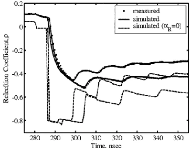
mea-sured waveforms and predicted waveforms using the inverted pa-rameters for both open-end and shorted-end conditions. The great match between the measured and predicted waveforms validates the TDR wave propagation model and the calibration by full-waveform inversion. The simulated full-waveform in which cable resis-tance is ignored is also shown in Fig. 4. The difference between this waveform and the measured one manifests the importance of ac-counting for cable resistance. The rise time and the steady-state re-sponse are greatly affected by long cables. Errors may arise in the analysis of travel time, steady-state response, magnitude of reflec-tion spike, or spectral response if the cable resistance is not taken into account. The following section will demonstrate the usefulness of the TDR wave propagation model for various geotechnical appli-cations.

Interpretation Based on TDR Wave Propagation Model

Interface and Dielectric Type Example

The dielectric property of the insulating material may vary along the transmission line in interface and dielectric type of applica-tions. The parameter of interest in an interface-type application is the position where dielectric property changes共e.g., groundwater level or scouring depth兲, while the dielectric property is to be deter-mined in the dielectric-type application where the interface is fixed. In general, waveform inversion based on the TDR wave propaga-tion model can simultaneously determine the interface and the

di-FIG. 4—Calibrating the cable parameters of a 30-m long RG58A/U cable by

matching the measured and simulated waveforms.

LIN AND TANG ON ACCURATE TDR MODEL 5

AQ: #1 PROOF COPY [GTJ100012] 003702GTJ

PROOF COPY [GTJ100012] 003702GTJ

PROOF COPY [GTJ100012] 003702GTJ

electric property. As an example, Fig. 5 shows the laboratory setup for water level monitoring. A water level sensing waveguide made of an air-dielectric coaxial cable共Andrew HJ5-50兲 was connected to the 30-m lead cable described in the preceding section. A TDR measurement with the sensing waveguide simply in air was taken for calibrating the transmission-line parameters共Zp,␧r

*_{, and␣} R兲 of

the connector and the sensing waveguide. The sensing waveguide was then inserted into a water-filled tube. Two measurements were taken for water levels at 20 cm and 30 cm from the cable end.

Traditionally, the tangent-line method can be used to locate the air-water interface. A line parallel to the horizontal axis is drawn tangent to the trace at a local minimum around the reflection. A second tangent is drawn at the point of maximum gradient after the local minimum of the TDR waveform. The intersection of this line with the horizontal line determines the reflection point of the inter-face 共Timlin and Pachepsky 1996; Klemunes et al. 1997兲. The water levels calculated by the tangent-line method are 22.31 cm for the 20-cm water level and 33.72 cm for the 30-cm water level. The discrepancy is attributed to the ambiguity of the empirical tangent-line method. As the cable length increases, the reflected waveform becomes smeared as a result of the cable resistance. Hence, water level cannot be accurately determined by the empirical tangent-line method.

Precise water level can be back calculated from the measured waveform using the wave propagation model with known transmission-line parameters 共Zps,␧rs

*_,␣

Rs兲 of the sensing

wave-guide. The sensing waveguide is divided into two parts, one filled with air and the other filled with water. The complex dielectric per-mittivity 共including the electrical conductivity兲 of groundwater may vary with temperature and contamination. Therefore, it is more general to treat␧_rw* 共complex dielectric permittivity of the water in the sensing waveguide兲 as an unknown. With the capability of full-waveform simulation, the water level and␧_rw* 共f兲 can be si-multaneously determined using the full-waveform inversion. In this case, the monitoring system is divided into three sections of uni-form transmission line: the lead cable, sensing waveguide in air, and sensing waveguide in water共see Fig. 5兲. For simplicity, the con-nector is considered as part of the lead cable. Parameters 共Ll, Zpl,␧rl*,␣Rl兲 and 共Ls, Zps,␧rs*,␣Rs兲 can be calibrated beforehand.

The remaining unknowns are Lswand␧rw

*_{. Since the dielectric}

re-laxation frequency of water is much higher than the TDR frequency range, dielectric permittivity of water can be considered frequency-independent in the TDR frequency range. The complex dielectric permittivity of the water can then be written as

␧rw * _{共f兲 = ␧} rw− j␴w 2␲f␧0 共9兲

where␧rwand␴ware the dielectric permittivity and electrical

con-ductivity of water, respectively.

Figure 6 shows the waveform matching when the inversion con-verged. Also shown for comparison in Fig. 6 are the simulated waveforms when cable resistance is ignored共␣R= 0兲. The resulting

estimations of water level共Lsw兲 were 20.01 cm for the 20-cm water

level and 30.48 cm for the 30-cm water level, respectively. In addi-tion,␧rw= 79.9 and␴w= 0.0323 S / m were obtained from the

inver-sion, which compares well with the expected values共␧rw= 80.2 and

␴w= 0.0323 S / m兲 determined by a three-prong TDR probe and

conductivity meter. This example demonstrates the effectiveness of the wave propagation model to infer from the TDR waveform both the interface of impedance mismatch and electrical properties of the material in the sensing waveguide. The interpretation of scour-ing and sediment monitorscour-ing may be treated similarly. When a multi-conductor waveguide or TDR penetrometer is used for soil measurements, the accurate wave propagation model also serves as a precise kernel for inverting dielectric spectrum of soils. Long dis-cussion of dielectric spectroscopy should be left for a separate paper.

Crimp Type Example

The cable is crimped when subjected to localized shear. Conven-tional data interpretation correlates amplitude of the reflection spike at the crimp with the localized shear deformation. However, the amplitude of the reflection spike is also greatly affected by the cable length and the width of the crimped zone. These factors can be effectively taken into account using the wave propagation model, as will be demonstrated on a direct shear test. Figure 7

illus-FIG. 5—Schematic of the laboratory setup for water level monitoring and the

associated multi-section transmission line model.

FIG. 6—Comparison of the measured and predicted TDR waveforms in water

level monitoring.

FIG. 7—Schematic of the laboratory setup for monitoring of localized shear

deformation and the associated multi-section transmission line model.

6 GEOTECHNICAL TESTING JOURNAL