利用方向小波轉換分析進行視訊編碼之位元分配

國

立

交

通

大

學

資訊工程學系

碩 士 論 文

利用方向小波轉換分析進行視訊編碼之位元分配

Curvelet Domain Analysis for Video Coding Bit Allocation

研 究 生：蔡雅婷

指導教授：蔡淳仁 博士

利用方向小波轉換分析進行視訊編碼之位元分配

Curvelet Domain Analysis for Video Coding Bit Allocation

研 究 生：蔡雅婷 Student：Ya-Ting Tsai

指導教授：蔡淳仁 Advisor：Chun-Jen Tsai

國 立 交 通 大 學

資 訊 科 學 與 工 程 研 究 所

碩 士 論 文

Submitted to Institute of Computer Science and Engineering College of Computer Science

National Chiao Tung University in partial Fulfillment of the Requirements

for the Degree of Master in

Computer Science June 2007

Hsinchu, Taiwan, Republic of China

利用方向小波轉換分析進行視訊編碼之位元分配

學生：蔡雅婷 指導教授：蔡淳仁博士

國立交通大學資訊科學與工程研究所

摘要

Curvelet Domain Analysis for Video Coding Bit Allocation

Student：Ya-Ting Tsai Advisor：Dr. Chun-Jen Tsai

Computer Science and Engineering College of Computer Science

National Chiao Tung University

Abstract

This paper proposes a video bit allocation scheme based on Curvelet domain analysis. The proposed algorithm analyzes the structural characteristics of the intensity and motion-compensated residual images of a video sequence in curvelet domain to determine a bit-allocation policy so that visually important regions will be allocated with more bits. Curvelet transform is adopted in this thesis for such analysis because it performs sub-band decomposition in various directions so that more structure information is revealed in curvelet domain than in DCT or other wavelet domains based on separable transforms. The proposed bit-allocation policy tries to save bits in unstructured regions and increase quality in structured regions. Experiments using standard test sequences coded with an MPEG-4 simple profile video encoder show that the proposed bit allocation method has better performance (achieves higher PSNR’s) in the regions most human observers care about in all test cases.

Acknowledgement

I would like to express my gratitude to all those who supported and encouraged me to complete this thesis. First of all, this paper owes much to the thoughtful and helpful suggestions and comments of my advisor, Professor Chun-Jen Tsai. I gratefully acknowledge helpful discussions with him on several points in the paper. Then, my special thanks are due to my seniors, juniors, and classmates, especially my senior, Chien-Peng Ho for consistent encouragement and valuable advice. During these days at National Chiao-Tung University, I enjoy the moments I have with all MMES Lab members. Finally, I would like to thank my dear parents and brother for their support and encouragement.

Content

TU

1.

Introduction

...1

TU

2.

Previous Work

...4

TU2.1.UT TUTransform AnalysisUT...4

TU2.2.UT TUProperties of Human Visual SystemUT...7

TU

3.

Study and Analysis of Curvelet Transform

...10

TU3.1.UT TUWhy Curvelet TransformUT...10

TU3.2.UT TUFundamentals of Curvelet TransformUT...11

TU3.3.UT TUMathematical Formulation of Curvelet TransformUT...13

TU3.4.UT TUImplementation of Digital Curvelet TransformUT...17

TU3.4.1.UTTUTake Fourier transform into frequency domainUT...18

TU3.4.2.UTTUBand-pass filteringUT...19

TU3.4.3.UTTUPolar interpolationUT...24

TU3.4.4.UTTUInverse Fourier transformUT...26

TU3.5.UT TUInterpretation of the Curvelet Transform CoefficientsUT...26

TU3.5.1.UTTUCurvelet Coefficients in the Coarsest and the Finest levelUT...27

TU3.5.2.UTTUCurvelet Coefficients in the Middle Levels of ResolutionsUT...27

TU

4.

Proposed Bit Allocation Framework

...30

TU4.1.UT TUAnalysis on curvelet transform coefficientsUT...30

TU4.1.1.UTTUThe composition of the curvelet transformUT...31

TU4.1.2.UTTUImage type and the presentation of the related coefficientUT...33

TU4.2.UT TUThe Otsu AlgorithmUT...35

TU4.3.UT TUStatistical method to analyze the coefficientsUT...38

TU4.4.UT TUProposed Bit Allocation SchemeUT...41

TU4.5.UT TUDetermination of the Weighting ThresholdUT...43

TU

5.

Experiment and Analysis

...46

TU5.1.UT TUResult of the proposed bit allocation schemeUT...46

TU5.2.UT TUResult of Proposed Bit Allocation Scheme with Weighting ThresholdUT...52

TU5.2.1.UTTUNumber of structured and unstructured blocks of the two methodUT...53

TU5.2.2.UTTUThe result of proposed scheme with linear formulaUT...54

List of Figures

TUFigure 2.1. Reduction of blocking artifacts using DCTUT...5

TUFigure 3.1 The anisotropy scaling relation for curves.UT...12

TUFigure 3.2 The curvelet tiling in the frequency domainUT...17

TUFigure 3.3 Decomposition of image into frequency domainUT...18

TUFigure 3.4 Decomposition of Meyer wavelet in resolution of scale 0 to scale 4UT...20

TUFigure 3.5 Scaling function and wavelet function of Meyer window functionUT...21

TUFigure 3.6 Angular scaling in the East quadrant regionUT...24

TUFigure 3.7 The directional decomposition in the 4UPU th UPU level coefficients.UT...26

TUFigure 3.8 Perform 2D IFFT on lowest levelUT...26

TUFigure 3.9 Result of coarest level of curvelet coefficientsUT...27

TUFigure 3.10 Coefficients of each resolution levelUT...28

TUFigure 3.11 Position mapping of curvelet coefficientsUT...29

TUFigure 4.1 Position mapping of curvelet coefficients in the coarsest level resolutionUT31 TUFigure 4.2 Curvelet coefficients in the finest level resolutionUT...32

TUFigure 4.3 Curvelet coefficients in the 2UPU nd UPU, 3UPU rd UPU and 4UPU th UPU level resolutionUT...32

TUFigure 4.4 Curvelet coefficients in the 2UPU nd UPU, 3UPU rd UPU and 4UPU th UPU level resolutionUT...34

TUFigure 4.5 The coordinate formed by curvelet coefficientsUT...35

TUFigure 4.6 The histogram separated by Otsu threshold selection methodUT...38

TUFigure 4.7 The histogram and coefficient of variation of six blocks in Stefan imageUT40 TUFigure 4.8 Block diagram of the proposed bit allocation modelUT...42

TUFigure 4.9 GOP structure of a video sequence.UT...45

TUFigure 4.10. Threshold selection of CV.UT...45

TUFigure 5.1 Comparison of visual quality in Stefan SequenceUT...49

TUFigure 5.2 Comparison of visual quality in Football SequenceUT...50

TUFigure 5.3 Comparison of visual quality in Bus SequenceUT...51

TUFigure 5.4 Comparison of visual quality in Stefan SequenceUT...56

TUFigure 5.5 Comparison of visual quality in Football SequenceUT...58

TUFigure 5.6 Comparison of visual quality in Bus SequenceUT...60

TUFigure 6.1 The directional decomposition in the 4UPU th UPU level coefficients.UT...63

List of Tables

TUTable 3.1 Input Parameter to curvelet codecUT 17

TUTable 3.2 Four basic parts of 1-D Meyer windowUT 22

TUTable 3.3 Parameters of each resolution levelUT 22

TUTable 3.4 The band-pass filtered coefficients of image LenaUT 23

TUTable 3.5 Formula of Meyer WindowUT 25

TUTable 4.1 Analysis of frequency components.UT 44

TUTable 5.1 Parameter settings of the three experimentsUT 47

TUTable 5.2 Resulted data of the three sequencesUT 47

TUTable 5.3 Ratio of improvement in Stefan sequenceUT 49 TUTable 5.4 Ratio of improvement in in Football sequenceUT 51 TUTable 5.5 Ratio of improvement in in Bus sequenceUT 52 TUTable 5.6 Automatic selection of threshold using method I.UT 53

TUTable 5.7 Automatic selection of threshold using method II.UT 54

TUTable 5.8 Average result of Method IUT 55

TUTable 5.9 Average result of Method IIUT 55

TUTable 5.10 Ratio of number of regions with better PSNR and worse PSNR in Stefan

sequenceUT 56

TUTable 5.11 Saved bits in unstructured regions in Stefan sequenceUT 57 TUTable 5.12 Ratio of number of regions with better PSNR and worse PSNR in Football

sequenceUT 59

TUTable 5.13 Saved bits in unstructured regions in Football sequenceUT 59 TUTable 5.14 Ratio of number of regions with better PSNR and worse PSNR in Stefan

sequenceUT 60

1. Introduction

Digital distribution of video is becoming popular today due to the applications such as digital television, digital camcorder, DVD player, etc. For the decades, video compression is an important technology in multimedia applications. A great number of digital video codec standards have been published; including MPEG-2, MPEG-4, and H.264, etc. Many research efforts have been put into the design of encoders that can achieves the best overall quality based on these standard codecs.

In video codec, the coding scheme can be divided into several processes: predictive coding, transform coding, quantization (e.g. rate-distortion coding), and entropy coding. Transform coding tries to decorrelate the components of video data and to centralize the energy of video data in order to facilitate rate-distortion coding and entropy coding. In recent years, many different transforms have been published to improve compression efficiency. Among these transforms, the most popular transforms are Fourier Transform, Discrete Cosine Transform (DCT) and Wavelet Transform.

Discrete Cosine Transform is more widely used for image and video coding than Fourier Transform since the performances of these two transforms are similar but the operation of DCT is simpler: DCT involves only real number operations instead of complex number operations. Wavelet Transform becomes more popular in recent years since it captures both frequency domain and spatial domain information in one compact representation. The wavelet transform performs very well on one dimensional signal since it can represent signal discontinuity in a more compact form than DCT does, but not as good as expected on two-dimensional data.. The main reason is that to reduce computational complexity, most practical wavelet transform implementation uses separable 1-D transform. The contours in a two-dimensional image can be oriented in any directions. However, the separable wavelet

transform only captures signal discontinuities in horizontal and vertical directions.

Recently, a new sub-band decomposition method called curvelet transform has been proposed. Unlike the wavelet transform, curvelet transform decomposes data components into multi-directional data sets and it also maintains the multi-scale spatial information similar to that of a wavelet transform. However, it is not easy to find a critically-sampled curvelet domain representation of an image, therefore, curvelet transform are not used for general image or video compression applications. It is more often used to separate high frequency components due to noises and high frequency components due to signal discontinuities of the image data.

In a video codec, the module that controls the size of the bitstreams for different coding units is called the rate control module. Finding a good trade off between video data rate and visual quality (distortion) is one of the key issues of a high performance rate control scheme. Most encoder tries to estimate the rate-distortion function of a video sequence during encoding. However, the distortion measures are usually MSE or MAD-based so that it does not precisely reflect the visual importance of the video data. In general, the importance of a coding unit is related to the sub-band data in the frequency domain. For example, the components of high-band frequency data are less visually important than the low-band frequency data at the same spatial resolution scale.

It has been shown X[19]XX[35]X that a structured-region in image has more visual importance

than an unstructured-region in image. A region full of random textures (or motion-compensated residuals in residual images) is usually hard to encode and not easy for human eyes to discern the degree of distortions. This kind of image component is referred to as unstructured regions. On the other hand, a region whose textures are simple, with discontinuities in only few directions is referred to as structured region, and any distortion in such regions can be picked up easily by human eyes.

In general, it is not easy to classify between structured and unstructured regions in an image, especially when the definition of “structureness” is dependent on human observers. In this thesis, the curvelet domain analysis is proposed to achieve this goal.

The major advantage of curvelet transform is to decompose input data into frequency coefficients of several directions at each spatial resolution scale. Therefore, in this thesis, we try to analyze video data in curvelet transform domain by its directional presentation in order to classify image regions into structured and unstructured regions and to achieve better bit allocation for video compression. The goal of the proposed technique is to save bits in unstructured regions since human eyes can not discern the distortion. The saved bit budget will be allocated to structured regions to improve its visual quality.

The organization of the thesis is as follows. Chapter 2 introduces some related work of rate control schemes and the perceptual models of human visual systems. Chapter 3 introduces the curvelet transform, including the mathematical definition and its architecture. In chapter 4, the proposed method will be described in detail. The experimental results will be shown in chapter 5. Finally, the conclusions and discussions will be given in chapter 6.

2. Previous Work

As mentioned in chapter one, the main purposes of the transform coding process are to find a more compact data representation and to facilitate video data analysis for rate-distortion coding. For several decades, a great number of different transforms has been studied. Among these transforms, the most popular transforms used for transform coding are the Discrete Cosine Transform (DCT) and the Wavelet Transform. However, since these transforms do not decompose the frequency sub-bands alone image edges, existing transform domain representations are not compact at signal discontinuities. A new transform, curvelet transform, tries to provide multi-resolution and multi-directional signal decomposition, is introduced by Cand`es et al.X[22]X X[23]XX[24]X. What is more, Human Visual System (HVS) is researched to

classify the regions in image whether the distortion of the region human eyes are sensitive to or not. These studies are of use in compression technique during the bit-allocation selection scheme.

The organization of this chapter is as follows. In section 2.1, we will first introduce popular transforms used in transform coding systems. And then we will analyze the pros and cons of existing transforms and briefly describe the reasons why a new transform, curvelet transform, is adopted in this thesis. In section 2.2, existing work on modeling the relation between human vision systems and the characteristics of images are discussed. Furthermore, the reason why we use curvelet analysis to distinguish between unstructured-texture regions and structured-texture regions are discussed.

2.1. Transform Analysis

For a long time, Discrete Cosine Transform (DCT) X[1]XX[2]X is one of the most popular

The DCT is defined as follows X[3]XX[4]X: j) f(i, 2N 1)v (2j cos 2M 1)u (2i cos MN C(u)C(v) v) F(u, M-1 0 i 1 -N 0 j π π + + =

∑∑

In equation 2.1, f(i, j) represents an entry of coefficients on the location of (i, j) and M and N mean the size in the horizontal and vertical direction separately. The two-dimensional DCT transforms it into a new function F(u,v), with integer u and v running over the same range as i and j. Equation 2.2 defines the value of multiplicator C(ξ) according to whether the DCT coefficient is the direct current (DC) component of the signal or not.

Compared to DFT, DCT can minimize the blocking artifact when coefficients are truncated or quantized. For example, as shown in Figure 2.1, the implicit n-point periodicity of the DFT can be replaced by the implicit 2n-point periodicity of the DCT. Therefore, the boundaries between adjacent sub-images become invisible because implicit 2n-point periodicity of DCT does not inherently produce boundary discontinuities.

n 2n

D D

In 1987, Mallat constructed a structure of wavelet function and the analysis and synthesis progress of signal decomposition. More importantly, Mallat first showed that wavelets are the foundation of a powerful approach to signal processing and analysis called multi-resolution theory X[7]X. In the next year, Daubechies proposed orthonormal and compactly supported

wavelet and the theory of wavelet analysis was constructed X[8]X.

The main advantages of wavelet transform are listed as follows. First of all, wavelet transform is computationally efficient and inherently local; therefore, it is not necessary to subdivide the original image into sub-images before applying the transform. As a result, the method eliminates the side effect of blocking artifact which is usually produced by the DCT-based compression scheme. Even more importantly, signals decomposed into wavelet domain have good resolution in both time and frequency domain. These characteristics work nicely for one-dimensional signals. Signals such as audio data using wavelet-based compression scheme perform better than those using the traditional DCT-based compression scheme. Finally, wavelet transform can decompose signals into coefficients with different levels of resolution, and the characteristic is called multi-resolution X[9]X. For analyzing the

signal data, multi-resolution representation is very effective since the decomposed coefficients are scale-invariant interpretations. These kinds of decomposition provide a hierarchical framework to interpret the signal data.

However, for two-dimensional image or video compression, traditional wavelet transforms which use 1-D separable transforms to decompose the sub-bands has significant drawbacks. Such transforms only capture signal discontinuity efficiently in either horizontal or vertical directions. Nevertheless, the direction of signal discontinuities in two dimensional signals can vary along 360 degree of angles. Traditional separable wavelet transform fails to capture the geometry of image and edges due to the fact that the directions of contours in

To remedy this shortcoming, another method of sub-band decomposition called curvelet transform has been published. Unlike the wavelet transform, curvelet transform not only decomposes data components into multi-direction data sets but also maintains the characteristic of multi-scale spatial resolution of wavelet transforms X[12]XX[13]X. In this thesis,

curvelet transform is used as a tool to help analyzing the contours of the two-dimensional images. The detail description of curvelet transform is presented in next chapter.

2.2. Properties of Human Visual System

In resent years, many researches on Human Visual System (HVS) are published, hoping to find a computational model for the behavior of human eyes X[14]XX[15]X. These researches are

important to image processing and coding X[16]XX[36]X.

When human observers look at still images, the perceptual importance of each region in images is not the same. Many characteristics of the image regions such as the shape of objects, the contrast of luminance, the location of objects, the size of the full objects, and the articulation of the objects will affect the perceptual importance significantly. Furthermore, whether an object is in the foreground or the background may also affect its perceptual importance X[17]X.

Many studies of the relation of human eye movements and the features have been published X[15]X-X[19]X. When humans look at a still image, they move their eyes several times a

second. Therefore, the features of the region that human eyes stop to gaze every time can be considered as the features that can attract human eyes. Enhancement of the visual quality of these regions is a higher priority task than improving other regions’. Some researchers classify the features of the regions that attract human eyes’ attention into three main groups. First, human observers always take priori notice of the regions that contain the faces X[18]X.

observers than other regions. Third, human eyes also tend to look at the regions that the correlations of the intensities of the nearby image pixels are weaker X[19]X.

The regions which have large contrast intensities include two different types of textures: the structured-textured regions and the unstructured-textured regions. More precisely speaking, these two kinds of regions can be discriminated by the representation of the edges (signal discontinuities) in the region. First of all, the structured region means that the number of the edges of objects inside the specific region is relatively little and the lengths of the edges are long (structured stimuli). On the other hand, the unstructured region means that the number of the edges of objects inside the specific regions is quite large, the position and the direction of the edges are quite random, and the lengths of the edges are small (random stimuli).

As a result, the distribution of edge pixels in unstructured region is scrambled and entropy of this kind of region is usually higher than that of the structured regions. However, human observers usually have trouble discerning the distortion in the unstructured regions. In other words, we can dispatch fewer bits to the unstructured regions because human eyes are less sensitive to its distortions. On the other hand, since human eyes are more sensitive to the distortions in the structured regions, allocating more bits to structured regions can enhance the visual quality more significantly than allocating more bits to unstructured regions.

For a video sequence, previous discussion on the structure of textures can be extended to the temporal domain as well. If the motion of an object from one frame to the next is smooth and can be tracked easily by eye movements, the texture of the object will have a stable projection on the retinas. Therefore, it would be easy for human to discern coding distortion of the sequence on this particular object. On the other hand, if the motion is random, it would not be easy for human eyes to get a stable image on the retina and the coding noises would not be apparent to a human observer. The type of motion can be analyzed from the

motion-compensated error residual images. Again, random, small edges in the error residual images around the area of the object means that the object is moving randomly, while an area with structured residual images means that the object is moving smoothly.

In this thesis, we propose a new model that can distinguish the unstructured regions from the structured ones. Therefore, the new model can be used in the bit-allocation process to enhance the visual quality of coded bitstreams.

3. Study and Analysis of Curvelet Transform

The goal of this thesis is to design a video bit allocation model based on visual behavior. As the previous chapter describes, we perform video data analysis in curvelet domain. Therefore, before we present the perceptual model-based bit allocation algorithm, we first introduce the 2-D curvelet transform in this chapter. First of all, we must study the theory and characteristics of curvelet transform. Secondly, it is important to understand the digital implementation of curvelet transform and the meaning of transformed coefficients in order to design the bit-allocation algorithm for perceptual-based video coding.

This chapter is organized as follows: We begin in section 3.1 by showing the reason why we must use curvelet transform to analyze the video data. Section 3.2 describes the main features of curvelet transform. In section 3.3, the mathematical formulation of curvelet transform is presented. Furthermore, section 3.4 presents the implementation of digital curvelet transform. Finally, the representation of transformed coefficients is introduced in section 3.5.

3.1. Why Curvelet Transform

For the last two decades, many transformations based on multi-scale decomposition have been published X[7]X-X[14]X. Today, especially in the field of signal processing, multi-scale and

multi-resolution based transformations such as wavelets are becoming the popular decomposition methods. Multi-scale transforms have many advantages X[21]X. First of all, with

multi-resolution transform, compressed data can be transmitted in scalable fashion. That is, low resolution data can be transmitted before high resolution data. Secondly, using multi-scale transform is convenient for data mining in large datasets. Thirdly, signal noise removal, for

example, in image restoration is more effective in the multi-resolution transform domain. As a result, there are an increasing number of studies of multi-scale and multi-resolution transformations recently.

In last few years, a multi-scale based transform, curvelet transform, was developed to improve the limitations of traditional multi-scale transforms.X[22]X X[23]XX[24]X Generally

speaking, the curvelet transform is applied using a pyramid structure with multi-resolution. In each scale of the pyramid, the curvelet coefficients records frequency components along different directions X[25]XX[26]X.

Comparing to traditional 2-D wavelet transform for images, curvelet transform is an over-complete system that contains more sub-band information and therefore it handles some problems better than traditional wavelets X[27]X. In curvelet transform domain, the

representation of edges in an image region (at a particular scale) can be analyzed from multi-directional decomposition of the spatial edges into frequency components. With multi-directional frequency decomposition and multi-resolution characteristics of the curvelet transform, we can obtain more information regarding the structure of the image textures (or the motion-compensated residuals). To be more specific, in the proposed bit allocation scheme, we first analyze the image data according to their frequency components along each edge direction. This analysis discriminates a region with structured texture (or motion-compensated residuals) from a region with unstructured texture (or motion-compensated residuals). Finally, the result of the analysis is used in the bit allocation decision in the video rate control mechanism. All the processes will be described in detail in next chapter.

3.2.

Fundamentals of

Curvelet Transform

which is also called the curve scaling law X[23]X.

2

length

width ∝ (3.1)

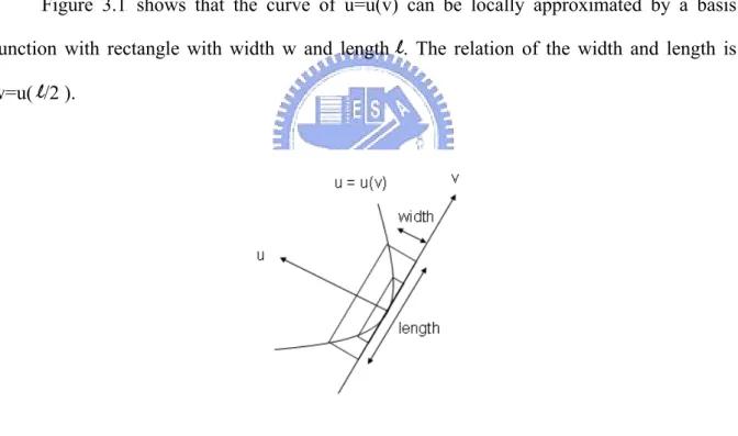
XFigure 3.1X illustrates the basic idea of curvelet transform X[23]XX[24]X. First of all, suppose

there exists a curve u = u(v) in the (u, v) orthogonal coordinate system. In general, we can use the Taylor series expansion to expand the equation u=u(v) as in Equation 3.2.

XFigure 3.1X shows that the curve of u=u(v) can be locally approximated by a basis

function with rectangle with width w and length l. The relation of the width and length is w=u( l/2 ).

( ) ( )

( )

( )

Figure 3.1 The anisotropy scaling relation for curves.

Moreover, since the v-axis is tangent to the curve at the origin (0, 0), the value of the u(0) and u’(0) is zero. As a result, we can obtain Equations 3.3 and 3.4.

( )

In conclusion, if we construct a correct multi-resolution scale for two-dimensional curves, we will get better approximations when the scale becomes finer.

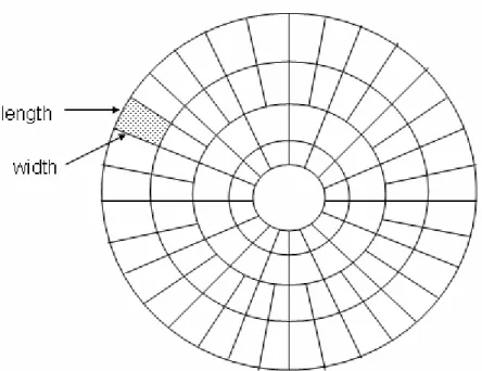
The advantage of curvelet transform comes from a flexible multi-resolution and directional image expansion using curve segments. To be more specific, curvelet transform is a multi-resolution decomposition method. If the total number of resolution is N, the 1P

st

P level

is the coarsest level and level N being the finest level N. Coefficients in the coarsest level and the finest level are not decomposed by directional filters, so they do not contain the information of directional frequency component analysis. On the other hand, coefficients from the 2P

nd

P level to the N-1P

th

P level are decomposed by two-dimensional band pass filter first and

then by directional filter latter. Therefore, for these levels, the coefficients will be separated by many angular wedges, and each wedge contains frequency components of the image signals decomposed along a specific orientation. The procedure of coefficients separation by angular wedges is called parabolic scaling.

3.3. Mathematical Formulation of Curvelet Transform

First of all, we define a two dimensional space, RP

2

P

, with four variables which are a spatial-domain variable x, a frequency-domain variable ω, and variables r andθin polar coordinates in the frequency-domain X[21]X. Conceptually, the principal filters are based on two

( )

∑

( )

∑

Equation 3.5 is the radial window W(r), which decomposes the image data in Fourier domain as the band pass filter. The window is smooth, nonnegative and real-valued, and its argument r is positive and real valued. Equation 3.6 is the angular window V(t), which decomposes the image data in Fourier domain into several wedges that contain different directional coefficients. The filter is also smooth, nonnegative and real-valued, and its argument t is real valued. The argument j represents the scale of the coefficients, and l means the direction of the coefficients.

( )

( )

The radial and angular window can form a frequency window UBjB as shown in Equation

3.7. Like Equation 3.5, the argument j represents the scale of the coefficient. To be more specific, jB0B is just the 1P

st

P level of the decomposition scale and

⎣ ⎦

In curvelet transform, the directional decomposition starts from the 2P

nd

P level of resolution and

ends at the last level of resolution. In other words, the 1P

st

P

level (coarse scale) decomposition can only produce the roughly low pass filtered coefficients. For other scales, UBjB can

decompose image data into polar wedges that contain different directions.

( )

(

)

( )

j r, U , U

U = = (3.8)

( )

( )

ϕˆ_j =U_j (3.9)

In Equation 3.8, we change the form of frequency window form polar coordinate to orthogonal coordinate. And then we can use the waveform in Equation 3.9 to define the frequency window.

Let’s introduce two parameters that indicate the position of coefficient in the polar wedge. ⎣ ⎦ π θ π θ 2 0 and 0,1,... ere wh , 2 2 - j/2 ≤ ≤ = ⋅ ⋅ = l l l l _(3.10) ( )

(

)

₍

₎

The Equation 3.10 expresses the rotation angles θBl Bthat we use to indicate the direction

of coefficients. The next Equation 3.11 shows the position of coefficient in the spatial domain that is controlled by the translation parameter k. And the notation is the inverse (and transpose) of rotation by θ radians as what Equation 3.12 shows.

( )j,k k

x

-1

R_θ

Therefore, at decomposition scale 2P

-j

P

, at the orientation of rotation anglesθBlB, and at the

position ( )j,k , basic curvelets can be defined as follows:

k

( )

(

(

)

)

As a result, we can use the inner product operation on an element f and a curvelet to produce a curvelet coefficient, and the formulation is represented as Equation 3.14.

(

)

( )

( )

( )

∫

We can also translate the curvelet coefficient of Equation 3.10 into the frequency domain operation as Equation 3.15 shows:

(

)

_{( )}

( )

( )

( )

( )

(

)

∫

∫

XFigure 3.2X shows the diagram of decomposition by curvelets in frequency domain. This

figure represents five decomposition level of resolution. The 1P

st

P level is the coarsest level,

which is only decomposed by low pass filter. Therefore, the 1P

st

P

level coefficients are non directional. Other levels are composed of angular wedges. The dotted region is one of the angular wedges in the 5P

th

P level coefficients. At scale 2P

-j

P, the length of each wedge is 2P

-j/2

P, and

the width of each wedge is 2P

-j

Figure 3.2 The curvelet tiling in the frequency domain

3.4. Implementation of Digital Curvelet Transform

In this section, we will describe the procedure for computing 2-D curvelet transform

X[21]XX[28]X. In short, the 2-D curvelet transform can be computed using unequally-spaced fast

Fourier transform (USFFT). The Fast Fourier Transform library used in the program can be obtained in X[29]X.

Some input parameters to the algorithm are described in XTable 3.1X, where nx and ny are

the input image width and height, and ns is the number of image resolution scale for wavelet decomposition, which is a result of logB2B(nx)-3. In addition, Meyer wavelet X[30]X is used for the

wavelet transform in the algorithm and nBϕB is the degree of the Mayer window function.

nx 512 ny 512 ns 6 nBϕB 3

Table 3.1 Input Parameter to curvelet codec

component Y. And then we use the Luma component Y as the input of the curvelet transformation. The procedure of computing curvelet transform is composed of four steps and each of the steps will be described in the following sections. Section 3.4.1 describes the Fourier transform procedure which transforms the image inputs into frequency components. Section 3.4.2 introduces the band pass filtering process that decomposes the frequency data into several resolution scales. The polar scaling method is described in section 3.4.3. Finally, section 3.4.4 shows how the coefficients are converted back to spatial domain via inverse Fourier Transform.

3.4.1. Take Fourier transform into frequency domain

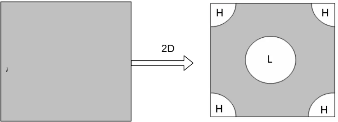
First of all, since we need to scale the image data by different resolution in the following steps, we must transform the image data into frequency domain. Assume that the input image data is in YCBBBCBRB format. To obtain Fourier samples of the image, a two-dimensional Fast

Fourier Transform is applied on the Luma components(Y channel of data), and the transform coefficients is normalized by dividing by (nx⋅ny)P

0.5

P. As XFigure 3.3X indicates, the low-band

coefficients are centralized in the center of the image since this representation facilitates repetitive decomposition of the coefficients.

n

n

2D

3.4.2. Band-pass filtering

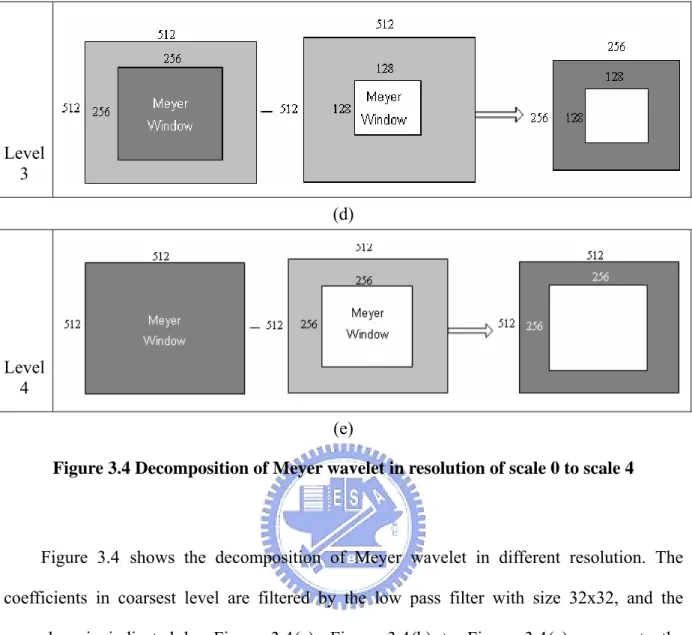
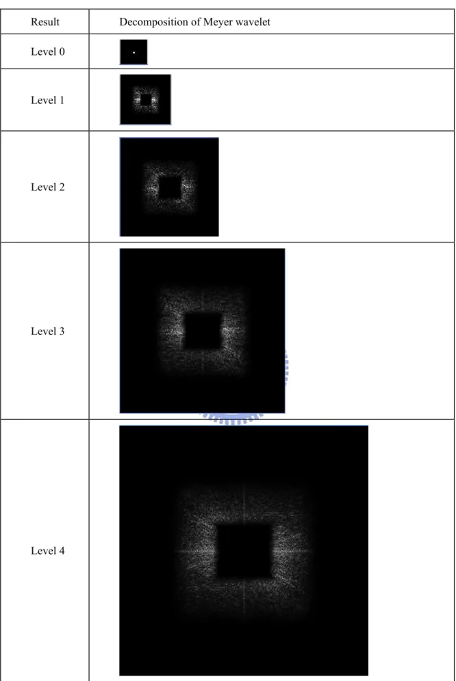
In the second step, we have to obtain frequency coefficients in different resolutions. First of all, we must create different levels of wavelet transform window function to decompose the coefficients obtained from previous step. XFigure 3.4X illustrates how the band-pass filters are

applied. Level 0 (a) Level 1 (b) Level 2 (c)

Level 3 (d) Level 4 (e)

Figure 3.4 Decomposition of Meyer wavelet in resolution of scale 0 to scale 4

XFigure 3.4X shows the decomposition of Meyer wavelet in different resolution. The

coefficients in coarsest level are filtered by the low pass filter with size 32x32, and the procedure is indicated by XFigure 3.4X(a). XFigure 3.4X(b) to XFigure 3.4X(e) represents the

coefficients in resolution of scale 1 to scale 4, respectively. For these scales, the filters are composed by the subtraction of two low-pass filters in order to form a band pass filters.

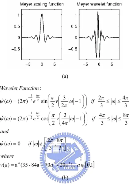
During the band-pass filtering procedure, the filters we apply are based on the low-pass Meyer window function. The scaling function and wavelet function of the Meyer window function is shown in XFigure 3.5XX[28]XX[30]X.

(a)

[ ]

Figure 3.5 Scaling function and wavelet function of Meyer window function

The detail procedure of decomposition is described as follows. First of all, we generate one-dimensional Meyer window of degree 3 by combining four basic parts, see XTable 3.2X.

The one-dimensional Meyer window is leading with a zero coefficient and then followed by the 4 parts with the order 4 3 2 1 2 3 4. Therefore, the one-dimensional Meyer window will be composed of [zero 4 3 2 1 2 3 4]. The two-dimensional Meyer window is constructed by point-wise multiplication of two one-dimensional Meyer windows.

Part The actual value of the filter 1 1…1

2 cos(πv/2(3a/2)) where a are dyadic points (2P

i+1 P/3…2P i P/3-1)/2P i P-1

3 cos(πv/2(3a/2))where a are dyadic points (2P

i P…2P i+1 P)/2P i P-1 4 1…1

Table 3.2 Four basic parts of 1-D Meyer window

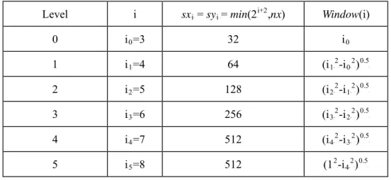
After generating the two-dimensional Meyer window, we filter the low frequency components by the Meyer window. To be more specific, the range of resulted low frequency components in resolution level i, sxBiB and syBiB, can be calculated by XTable 3.3X. The filter

coefficient we use in level i, where i are 1 to 4, is the square of coefficient i minus square of coefficient i-1, and then get its square root. In level 5, we use the coefficient of square roots of 1 minus square of coefficient 4. After the decomposition, we can get six different scales with size sxBiB·syBiB.

More over, the size of the coefficients is controlled by the level of their scale. And the relation of size and scale can be show as XTable 3.3X. To be more specific, sxBiB and syBiB are width

and height of level i.

Level i sxBiB = syBi B= min(2P i+2 P,nx) Window(i) 0 iB0B=3 32 iB0B 1 iB1B=4 64 (iB1PB 2 P-iB0PB 2 P)P 0.5 P 2 iB2B=5 128 (iB2PB 2 P-iB1PB 2 P)P 0.5 P 3 iB3B=6 256 (iB3PB 2 P-iB2PB 2 P)P 0.5 P 4 iB4B=7 512 (iB4PB 2 P-iB3PB 2 P)P 0.5 P 5 iB5B=8 512 (1P 2 P-iB4PB 2 P )P 0.5 P

Table 3.3 Parameters of each resolution level

Result Decomposition of Meyer wavelet Level 0 Level 1 Level 2 Level 3 Level 4

3.4.3. Polar interpolation

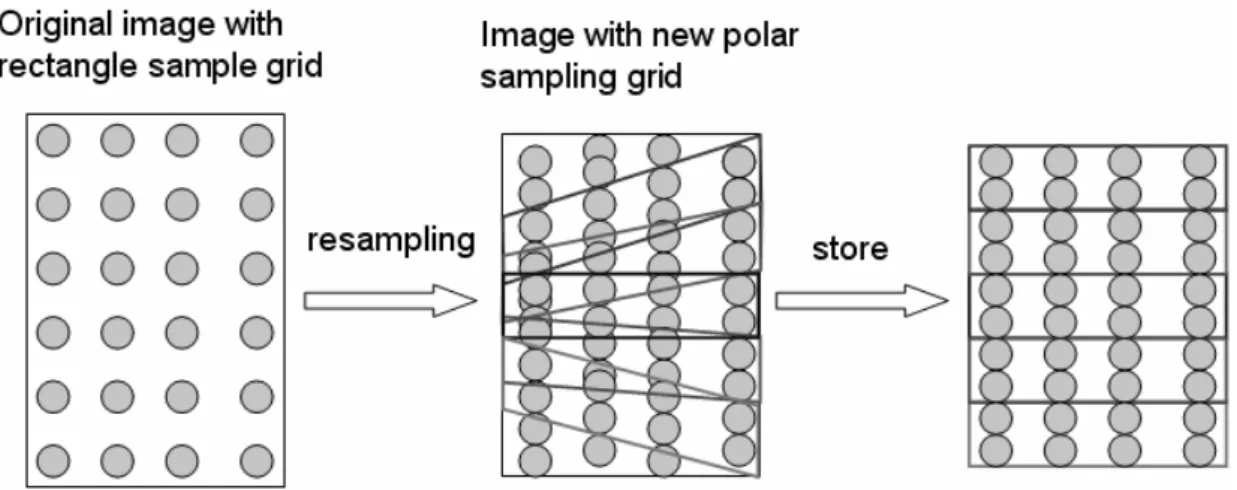
The frequency coefficients in different resolutions computed by the band pass filter must be re-sampled to form directional frequency components. This can be done by interpolating the coefficients obtained from the previous procedure along vertical and horizontal directions. After resampling, the coefficients may be rearranged into four groups, namely west, east, north and south, based on the directions of directional decomposition.

For example, for the coefficients in the east quadrant, the whole procedure of the directional decomposition is shown in XFigure 3.6X.

Figure 3.6 Angular scaling in the East quadrant region

First of all, we can obtain the rectangle shaped coefficients in the East quadrant. Secondly, we apply column-wise one-dimensional inverse Fast Fourier Transform on the coefficients. And then we have to resample the coefficients into a shape of wedges (shown in the middle picture in XFigure 3.6X). From XFigure 3.6X, one can see that, for each column, x

sampling gird stays the same, but y sampling grid must be rearranged along each column. Therefore, we have to calculate the new indices and interpolate the new coefficients. We obtain the new indices by performing a one-dimensional Meyer Window, see Table 3.5.

Meyer window is combined by the 4 parts Part 1 sin(πv/2(3a)) Part 2 sin(πv/2(3a)) Part 3 cos(πv/2(3a)) Part 4 cos(πv/2(3a))

Table 3.5 Formula of Meyer Window

Furthermore, the interpolation method is calculated by one sine window such as Equation 3.16. Finally, the resampled coefficients is stored in a rectangular shape region in transform domain for the purpose of easy accesses.

)))) 2 1 ( sin( 1 ( 4 sin( )))) 2 1 ( sin( 1 ( 4 sin( w = π + π t+ ⋅ π + π −t (3.16)

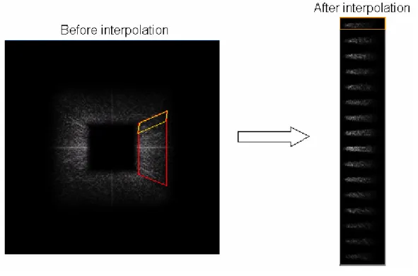
Note that for the east and west groups of coefficients the interpolation is done column-wise while for north and south groups of coefficients, the interpolation is done row-wise. XFigure 3.7X shows the coefficients before and after the procedure of the directional

decomposition. Coefficient in the right part is the result of the red ladder shaped region (East quadrant) in the 4P

th

P level resolution after applying the polar interpolation. To be more specific,

Figure 3.7 The directional decomposition in the 4P

th

P level coefficients.

3.4.4. Inverse Fourier transform

In the final step shown in XFigure 3.8X, two-dimensional Inverse Fast Fourier Transform is

applied on the coefficients to transform the data back to spatial domain. The pixel data is normalized by multiplication with (nx⋅ny)P

0.5

P in order to cancel the original normalization we

apply on the coefficients.

Figure 3.8 Perform 2D IFFT on lowest level

3.5.

Interpretation of

the Curvelet Transform

Coefficients

In this section, we will give an interpretation to the curvelet coefficients in each level of resolution. The coefficients at the coarsest and the finest levels are not decomposed along

different directions while the coefficients at other levels are decomposed along different angles.

3.5.1. Curvelet Coefficients in the Coarsest and the Finest level

As previous paragraph describes, the curvelet in the coarsest and the finest level of resolution do not contain the information of directional decomposition. To be more specific, the coarsest curvelet coefficients are the low-pass coefficients, and on the contrary, the finest curvelet coefficients are the high-pass coefficients.

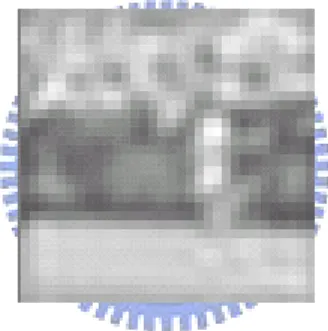
Here we show an example of coarset level curvelet coefficients by stefan image with size 352×288. Size of the coarset level curvelet coefficients is 32×32. After normalizing the coarest level of curvelet coefficients, the image of coefficients is shown in XFigure 3.9X.

Figure 3.9 Result of coarsest level of curvelet coefficients

3.5.2. Curvelet Coefficients in the Middle Levels of Resolutions

Curvelets in the middle levels of resolution contain the information of directional decomposition. For each resolution scale, the coefficients in different directions (within a wedges area along different angles) are resampled according to their orientation. The number of angles analyzed at one scale is chosen by the resolution of the scale. For instance, there are 32 different angular wedges in the 2P

nd

P and 3P

rd

P levels, and 64 different angular wedges in the

4P

th

P and 5P

th

P levels.

As other multi-resolution based transforms, curvelet coefficients can be presented in a spatial image. XFigure 3.10X (a) helps to define the position of curvelet coefficients. In the first

step, we allocate the coefficients of the coarsest level in the middle of image. In the second step, the coefficients of one scale are separate in to 4 parts composed of North, East, South and West. More over, we separately put the coefficients around the coarsest level coefficients from low level to high level. XFigure 3.11X shows the actual curvelet coefficient in 4 levels of

resolution of the Stefan image.

(a) (b)

Figure 3.10 Coefficients of each resolution level

Moreover, an example of the mapping between the positions of the curvelet coefficients and the original image pixel position is illustrated in XFigure 3.11X. The mapping function of the

coarsest-level coefficient is simple since it is just a subsampled version of the original image. However, the mapping of the other levels of coefficients is not as trivial since their samples are rearranged in the frequency domain. However, one can still derive the mapping function precisely by inversing the band pass filtering and the coefficient storage procedure described in this chapter. More details of the mapping function will be discussed in next chapter.

4. Proposed Bit Allocation Framework

In order to design a video bit allocation policy that matches human perceptual behavior, we must design a measure to distinguish between structured and unstructured regions (or motion-compensated residuals). The texture structure can be classified by analyzing the distribution of the angular frequency components in the curvelet domain. In the proposed framework, the analysis is done by classification of the histogram of frequency components across different angles. The assumption is that for a structured region, the histogram should have clear peaks (large magnitude frequency components) at few angles. On the other hand, for an unstructured region, the histogram will be nearly uniformly distributed.

The organization of this chapter is listed as follows. In section 4.1, some analyses on curvelet coefficients at different resolutions are presented. In section 4.2, we describe the Otsu thesholding algorithm, which is used in the proposed framework for histogram classification. Section 4.3 formulates the proposed statistical measure that calculates the degree of texture structure randomness in a specified region. Finally, section 4.4 presents the proposed bit allocation scheme for MPEG-4 simple profile.

4.1. Analysis on curvelet transform coefficients

Although curvelet transform provides decomposed frequency components at different resolutions, the coefficients at the coarsest and the finest resolutions do not arrange frequency components according to the direction of the transform windows. In this thesis, these coefficients are referred to as the first group of coefficients. The second group contains coefficients at other intermediate resolutions. These coefficients are arranged according to the direction of the transform windows. In section 4.1.1, we will describe the detail information of the curvelet coefficients in the two groups. In section 4.1.2, we will show the spatial

mapping between the original image positions and the corresponding curvelet coefficients.

4.1.1. The composition of the curvelet transform

We have glanced at some features in section 3.5. In this section, we will put more emphasis on the meaning of coefficients in a curvelet domain image and their relation to the original image.

First, we explain the components in the first group that do not contain the information of directional decomposition. For the coarsest-level coefficients, they contain the low frequency components and the size is diminished into fixed size of 32×32 pixels. Therefore, the position mapping between the original image and the transformed coefficients is a direct down-scale.

Figure 4.1 Position mapping of curvelet coefficients in the coarsest level resolution

Let’s take the simple edge image that the only edge starts from right-up corner to left-bottom corner as an instance. XFigure 4.1X shows the way of position mapping between

curvelet coefficients in the coarsest level resolution and the original image. The image of normalized coarsest coefficients is listed left whose size is 32×32 pixels, and the original image is listed right whose size is 352×288 pixels. We can easily find out the original spatial properties are remained in the curvelet coarsest level coefficients. Similarly, XFigure 4.2X is the

image of normalized finest level coefficients. Curvelet coefficients in the finest level resolution are the collection of high frequency components of the original image, and their total size is the same as the original image. Therefore, the positional mapping is direct

one-to-one mapping. In the proposed bit-allocation method, neither coefficient in the coarsest nor finest level of resolutions is used.

Figure 4.2 Curvelet coefficients in the finest level resolution

For the second group of coefficients that contain the information of directional decomposition, the number of levels depends on the original image size. For example, if the original image has 352×288 pixels, we can obtain three middle levels of resolution which are the 2P nd P level, 3P rd P level and 4P th P

level respectively, see XFigure 4.3X.

Figure 4.3 Curvelet coefficients in the 2P

nd P, 3P rd P and 4P th P level resolution For the 2P nd P and 3P rd

P level, coefficients are separated into 32 angles. However, there are 64

angular wedges in the 4P

th

As XFigure 4.3X shows, because the original image contains only an edge starts from the

right-up corner to the left-down corner, we can easily find out the coefficients are centralized in the region of left-up and right-down. In short, curvelet coefficients centralize the energy into the orthogonal angles of direction of the curves.

More over, the position mapping function of the middle levels is different from that of the first group. In section 3.5.1, as XFigure 3.11X shows, we have glanced at the relation of

positions between the curvelet coefficients and the original image. Because the directional decomposition process re-samples the coefficients in the frequency domain, and the direction of re-sampling varies according to the specified angles, the actual positions of the final coefficients are shifted in some direction. We can classify the directions of shifting into two groups. First, for East and West quadrants, coefficients in the vertical direction are simply proportional, but coefficients are shifted by the angle of the orientation in the horizontal direction. Secondly, for North and South quadrants, coefficients in the horizontal direction are simply proportional, but coefficients are shifted by the angle of the orientation in the vertical direction.

4.1.2. Image type and the presentation of the related coefficient

As XFigure 4.3X shows, we can easily understand the distribution of the curvelet

coefficients. Since the original image only contains a simple edge, the positions where the coefficient appears are simple, too.

Let’s see a more complex example. If the original image contains multiple multi-directional edges, such as the image in XFigure 4.4X(a), the distribution of its coefficients

(a) (b)

Figure 4.4 Curvelet coefficients in the 2P

nd P, 3P rd P and 4P th P level resolution

In XFigure 4.4X(b), we can see that the coefficients are distributed in multiple angular

wedges. Furthermore, it is natural that the angular wedges which the coefficient appears are different in each resolution. Therefore, curvelet transform can determine whether the curves in an image are complicated or not according to the directional decomposition in the middle levels of resolutions.

In our proposed scheme, we take each angular wedge in each resolution scale as a data unit. The actual process is to calculate the magnitude of one angular wedge in one resolution, and the magnitude becomes the representative value of the energy in the orientation in the resolution. Secondly, since we can get three resolution scales with directional decomposition, the coordinate formed by the magnitudes can be shown as in XFigure 4.5X.

Figure 4.5 The coordinate formed by curvelet coefficients

It is a three dimensional coordinate which is formed by the scale, magnitude, and angle. The angle indicates the angle of the orientation which starts at 0∘and ends at 360∘in the direction of clockwise. However, the total angles in each resolution scale are different. To be more specific, the 2P

nd

P, 3P

rd

P level resolution contains 32 angles respectively, but the 4P

th

P level

resolution contains 64 angles. In the plane of angle θand magnitude, we can see the figure as histogram. Naturally, value of the magnitude is according to its quantity of coefficient in the orientation. If the value of magnitude is larger, it means more data in this direction. Therefore, we can analyze the composition of histogram to see whether the direction in the image is structured image or not.

As a result, we can take advantage of the property in curvelet transform to analyze the input video data in our proposed bit-allocation scheme. In next section, we will introduce the Otsu algorithm to help analyzing the curvelet coefficients for the sake of determine whether a small area in an image contains complicated curves or not.

4.2. The Otsu Algorithm

For picture processing, the technique of selecting histogram threshold is very useful for many applications, such as object extraction or edge detection X[31]X. Therefore, there are a

variety of techniques proposed for threshold selection. In this section, we will introduce a typical threshold selection algorithm from gray-level histograms. The method is proposed by

Nobuyuki Otsu in 1979 X[32]X.

Generally speaking, given a histogram of an image, there is a deep and sharp valley between every two neighbor peaks. The position of the bottom of each valley is the threshold we want to obtain. In the algorithm proposed by Otsu, the histogram threshold can be derived form the viewpoint of discrimination analysis.

First of all, we assume the number of gray level in an image is L. The total number of pixels N is the summation of nBiB for level i=1, 2,…, L. The probability distribution is as

Equation 4.1 shows:

∑

Secondly, we can separate all pixels into two classes by a threshold at level k. CB0B is the

group which contain the pixels with level 1 to level k, and CB1B contain the pixels with level

k+1 to level L. The probabilities of class occurrence of CB0B and CB1B are listed in Equation 4.2.

(k) -1 p ) Pr(C p (k) e wher (k) p ) Pr(C L 1 k i i 1 1 k 1 i i k 1 i i 0 0 ω ω ω ω ω = = = = = = =

∑

∑

∑

Moreover, the probabilities of class mean levels of CB0B and CB1B are listed in Equation 4.3.

(k) -1 (k) -/ ip ) C | Pr(i i p i (k) re whe (k) (k)/ / ip ) C | Pr(i i T 1 L 1 k i i L 1 k i 1 1 L 1 i i 0 k 1 i i k 1 i 0 0 ω μ μ ω μ μ ω μ ω μ = = = = = = =

∑

∑

∑

∑

∑

( )

∑

Based on the formula and variable above, we can introduce the discriminate criterion measure, between-class variance, in Equation 4.5 to evaluate the threshold k X[33]X.

(

)

(

)

(

)

Since we can assume that if the two classes are distinguished by good threshold, the number of between-class variance must be large. Therefore, we can easily obtain the conclusion that the best threshold that separates the two groups must derive the maximum between-class variance over other thresholds. This relation can be formulated in Equation 4.6 where kP

*

P is the best solution of histogram threshold.

(k) max ) (k 2 B L k 1 2 B σ σ < ≤ = ∗ _(4.6)

Furthermore, the method can easily be extended into a multi-threshold case. Equation 4.7 shows the example of two-threshold selection method which can produce four peaks in the gray-scale histogram. L]. , 1, [k for C ], k , 1, [k for C ], k , [1, for C where ) k , (k max ) k , (k 2 2 2 1 1 1 0 2 1 2 B L k k 1 2 1 2 B 2 1 ⋅⋅ ⋅ + ⋅⋅ ⋅ + ⋅⋅ ⋅ = ∗ ∗ < < ≤ ∗ ∗ _σ σ (4.7)

In the previous section, we know that the input histogram is the curvelet coefficient in one resolution scale. The level indicates the angle of the angular wedges. In other words, the input data is the histogram of 32 or 64 level histogram. XFigure 4.6X(a) represents the result of

histogram into two groups.

(a) (b)

Figure 4.6 The histogram separated by Otsu threshold selection method

Furthermore, in our proposed scheme, we extend the threshold selection method to five-thresholds. As a result, we can obtain six classes in the whole histogram. And then as

XFigure 4.6X(b) shows, we will compute the value of the peak in each class. As a result, the rise

and fall of each histogram is different according to its composition of data in each orientation. We can assume that if the variety of histogram is bigger, the direction of edges in the image is more complicated. Therefore, we can use the six mountain peaks in the histogram to indicate the degree of complication of the image. The actual computational method is described in the continuous section.

4.3. Statistical method to analyze the coefficients

T

In the section, we use the coefficient of variation to measure the degree of variation of our histogram. The coefficient of variation (CV), which is also called “relative variability”, is a Tmeasure of dispersion of a probability distribution X[34]X. To be more specific, CVT represents

the ratio of standard deviation to the mean value.

TWe do not useTTTstandard deviation to analyze our data because has interpretable meaning

under the condition that the mean value of every sample is the same. In other words, standard deviation represents the degree of variability relative to the mean value. However, in our

different. Therefore the coefficient of variation is used instead.

(

)

∑

∑

Equation 4.8 shows the formula of the coefficient of variation (CV). It is easily seen that CV is the value the standard deviation divided by the mean. The measurement of the coefficient of variation is better in datasets with markedly different means or with different units of measurement. Our input dataset just match the first type.

Here we list six classical examples of histogram and its coefficient of variation in XFigure

4.7X. We take one residual frame of Stefan sequence with resolution CIF as our example. First

of all, we divided the image into 396 blocks with size 16 by 16. Therefore, we can obtain curvelet histogram of each block in each resolution level.

(c)

Figure 4.7 The histogram and coefficient of variation of six blocks in Stefan

Figure 4.7(a) shows actual positions of blocks we select. In Figure 4.7(b), it lists the coefficient of variation of each block in each level. To be more specific, cv1 means the coefficient of variation of the first level with directional decomposition, and cv2 means the coefficient of variation of the second level with directional decomposition, etc. And the curvelet histogram of the relative block is presented in Figure 4.7(c). As the histogram shows, one can see that the value of variation and the number of peaks exist some relation. Based on the number of peaks and the magnitudes of peaks in the histograms, the image region can be classified into several types of images. The first type is that the region doesn’t contain any clear edges at all, such as block 31, and the second type is that the region contains many small edges, such as block 24 in the first resolution level with directional decomposition. Both these two kinds of images are considered as unstructured image since their texture has complex

image

X X X X

it means that the distribution of the edges in the block is simple and clear. For example, block 145, 167, and 280 in the third resolution level shows such case.

4.4. Proposed Bit Allocation Scheme

The bit allocation algorithm st determines the quantization parameter

, we analyze the for video coding mu

based on the visual importance of a coding block. The input to the bit-allocation algorithm is a macroblock of video data. For intra-coded blocks, the input data is the image pixels while for inter-coded blocks, the input data is the motion-compensated error residuals. After curvelet transform, one can obtain the coefficients that are separated by their direction of contour and resolution. And then we can directly take each angular wedge in each resolution scale as a data unit as described in section 4.1. To be more specific, we integrate the coefficients by calculating the magnitude of one angular wedge in one resolution, and the magnitude becomes the representative value of the energy in the orientation in this resolution. As a result, the display of curvelet coefficients can be expressed as in XFigure 4.5X a three

dimensional coordinate which is formed by the scale, magnitude and angle. Next, as described in section 4.2, for each plane of angle and magnitude

mountain peaks of the histogram. Each mountain peak represents the gathering of direction of edges. To classify the complexity of the region, the coefficient of variation (CV) to analyze the mountain peaks of the angular histogram. On one hand, if the value of each mountain peak in one histogram varies slightly, it will be represented by a small CV and it means that the direction of edge in the block is not obvious. Of course we can indicate the image as an unstructured region. On the other hand, if the value of each mountain peak in one histogram varies dramatically, it will be represented by a large CV. It means that the direction of edge in the block is obvious, and we can indicate the image as a structured region.

In the proposed method, we separate all images into three groups. They are group of unstructured regions, group of structured region, and group of well structured regions. Since human eyes are less sensitive to images of unstructured regions than images of structured regions, we can adjust the way of bit allocation according to our analysis of the image. As a result, images of unstructured regions can be seen as unimportant regions, so we can diminish bits of the regions in a compression technique. On the other hand, we can increase bits of the well structured regions in order to enhance the performance of compression.

XFigure 4.8X shows the block diagram of the proposed bit allocation algorithm. Blocks in

the first line is the original encoding procedure of an MPEG-4 simple profile encoder, and blocks in the second line is the modified encoding flow.

Residual Image Quantization Curvelet Transform Distribution Analysis Adjust QP by CV of Peak Computation Blocked-DCT Transform Coding Entropy

Figure 4.8 Block diagram of the proposed bit allocation model

In the process of determining the complexity of images and adjusting QP based on the CV of histogram peaks, Equation 4.8 is proposed.

CV of maximum the is CVmax where 0.5) -T -T T -CV round( d min maxu min max QP =

If dBQPB is equal to 1, then check the minimum of CV:

If CVBminB is smaller then TBmaxlB, then change the value of dBQPB from 1 to 0

In Equation 4.8, TBminB controls the boundary of decreasing QP. If the maximum

coefficient of variation in three resolution levels (CVBmaxB) is less than TBminB, the macro block is

considered unstructured region, and QP of the macro block is reduced.

On the other hand, the way to judge whether the macro block is a strictly structured region or not is similar but contains one extra condition. TBmaxuB and TBmaxlB control the boundary

of increasing QP. If the maximum coefficients of variance (CVBmaxB) is larger than TBmaxuB and

minimum coefficients of variance (CVBmin.B) is not less than TBmaxlB, the macro block is

considered strictly structured region, and QP of the macro block is increased.

By using the formula to computing updates of quantization parameters for each macroblock, we can obtain three kinds of updated quantization parameters. The first group of quantization parameter is the same as the original quantization parameter. This means that the composition of image is a normally structured region, and we do not have to increase or decrease its bits. The second group of quantization parameter corresponds to the original quantization parameter plus one. This type of regions means that the composition of image does not contain obvious edges, so it is typically unstructured regions. We can decrease its bits and the compression result does not cause obvious degradation to human eyes. In addition, we can allocate the saving bits to other regions that the human observers are more sensitive to. And this is the behavior of the third type. The third group of quantization parameter equals the original quantization parameter minus one. This type of regions means that the composition of image contain clear edge structures, which is referred to as well structured regions. Therefore, we can increase its bits to enhance performance by human eyes, since the improvement of visual quality in this kind of region can dramatically catches human eyes.

4.5.

Determination of the Weighting Threshold

In the section, the selection of thresholds mentioned in previous section is described. In general, the degree of presentation of signal discontinuity contains a relationship to the

sampling frequency. Therefore, in order to consider the weighting of each resolution scale, we must analyze the range of minimum and maximum sampling frequencies in each directional resolution scale as listed in XTable 4.1X .

Min Max Scale Direction F (cycles/samples) T (cycle) F (cycles/samples) T (cycle) Horizontal 16/352 22 32/352 11 1 Vertical 16/288 18 32/288 9 Horizontal 32/352 11 64/352 5.5 2 Vertical 32/288 9 64/288 4.5 Horizontal 64/352 5.5 128/352 2.75 3 Vertical 64/288 4.5 128/288 2.25

Table 4.1 Analysis of frequency components.

From XTable 4.1X, one can see that the proportions of mean frequencies in these three

scales are 1:2:4. Consequently, the formula for the overall CV (combining information form all resolution scales) is computed as in Equaltion 4.1. Note that the sum of the coefficients is one and CVB1B, CVB2B, and CVB3B are the CV’s for different resolution scales.

3 2 1 0.29 CV 0.57 CV CV 0.14 CV= ⋅ + ⋅ + ⋅ (4.1)

Next, we must determine the threshold CV for structured and unstructured regions. The threshold is estimated by a pre-analysis step for each group of picture (GOP). One example of GOP structure which contains nine frames is shown in XFigure 4.9X.

Figure 4.9 GOP structure of a video sequence.

Two possible methods are tested to determine the CV threshold at a particular scale. Both methods are based on estimating the boundaries between well structured regions (SR) and unstructured region (USR).

Method I: the threshold of SR is computed as the value of CV that makes the regions with top 1/3 CV values being counted as well structured regions. Then, the threshold for the unstructured regions is selected so that it decreases the bitrate for the unstructured regions (nB1B%) so that the overall bitrate stays the same.

Method II: the threshold for SR is computed as that in method I, and the threshold for USR is determined so that blocks of the last nB2B% number are considered as USR.

(a)

(b)