Application example for evaluating networks considering correlation

A

PPLICATION

E

XAMPLE FOR

E

VALUATING

N

ETWORKS

C

ONSIDERING

C

ORRELATION

By Wei-Chih Wang

and Laura A. Demsetz

ABSTRACT: Current approaches to network scheduling do not consider the correlation between activity dura-tions. When activity durations are correlated, the variability of path and project durations may be increased. High variability in a project’s duration increases the uncertainty of completing the project by a target date. The model NETCOR (NETworks under CORrelated uncertainty) has been developed to evaluate schedule networks when activity durations are correlated. The NETCOR model builds upon a factor-based procedure to indirectly elicit correlation. An activity duration model disaggregates the effect of uncertainty by factors from a duration distribution (grandparent) for each activity. Correlation is captured by a child-distribution approach that further breaks down the factor-subdistribution (parent) based on the factor conditions. This paper demonstrates the practical application of NETCOR to a current construction project. Using the same inputs, the program evaluation and review technique and several simulation analyses that do not consider correlation also are evaluated. Com-parison of the results shows the significance of considering correlation in scheduling analysis.

INTRODUCTION

The critical-path method (CPM) is an accepted tool for plan-ning, scheduling, and monitoring construction projects. Basic CPM relies on the use of independently entered values for the durations of different activities. However, factors such as weather, labor skills, site condition, or management quality may affect the durations of many activities in a construction project. When a particular factor has a similar effect on several activities, the durations of these activities will be correlated; that is, they will tend to vary together. This correlation effect may result in an increase in the variability of path and project durations. High variability in a project’s duration increases the uncertainty of completing the project by a target date.

Other than manually adjusting activity durations to carry out a ‘‘what-if’’ analysis, basic CPM cannot reflect the fact that durations of multiple activities may vary together. To incor-porate correlation in scheduling analysis, previous research has relied on simulation-based or rule-based models (Wang 1996; Wang and Demsetz 2000). The common limitation of these models is their requirement of a ‘‘matching relationship’’ be-tween the outcomes of factors and activity duration samples to capture correlation. Such relationships are not available in practice. To relax this limitation, a simulation-based model, NETCOR (NETworks under CORrelated uncertainty) was de-veloped (Wang 1996).

In NETCOR, the impact of each factor on activity duration is qualitatively estimated by the user. Based on these qualita-tive estimates, the overall uncertainty in activity duration is disaggregated by factors. The uncertainty associated with a particular factor (e.g., weather) is further disaggregated based on the factor condition (e.g., better-than-expected, expected, or worse-than-expected weather). Correlation is introduced by selecting a factor condition (e.g., worse-than-expected weather) for a particular iteration and sampling for the dura-tion distribudura-tions associated with that condidura-tion for each ac-tivity.

The details of NETCOR are described in Wang (1996) and

1

Asst. Prof., Dept. of Civ. Engrg., Nat. Chia-Tung Univ., 1001 Ta-Hsueh Rd., Hsin-Chu 300, Taiwan.

2

Assoc. Prof., Engrg. Dept., Coll. of San Mateo, 1700 W Hillside Blvd., San Mateo, CA 94402-3784.

Note. Discussion open until May 1, 2001. Separate discussions should be submitted for the individual papers in this symposium. To extend the closing date one month, a written request must be filed with the ASCE Manager of Journals. The manuscript for this paper was submitted for review and possible publication on February 28, 1997. This paper is part of the Journal of Construction Engineering and Management, Vol. 126, No. 6, November/December, 2000.䉷ASCE, ISSN 0733-9634/00/0006-0467–0474/$8.00⫹ $.50 per page. Paper No. 15245.

Wang and Demsetz (2000). This paper illustrates the appli-cation of NETCOR to a current construction project. The NETCOR model is first reviewed, and then the construction project and NETCOR inputs are presented. NETCOR outputs are compared with the results of a program evaluation and review technique (PERT) analysis with several simulation analyses that ignore correlation. A summary and suggestions for further work complete this paper.

REVIEW OF NETCOR MODEL

The NETCOR model is built upon a factor-based proce-dure that indirectly elicits correlation. A brief review of the NETCOR model is presented here. A detailed description of the model can be found in Wang (1996) and Wang and Dem-setz (2000).

In NETCOR, the duration of an activity is modeled as the sum of a deterministic base duration and a series of zero-mean subdistributions resulting from the factors responsible for cor-relation. The overall activity duration [see the left side of Fig-ure 1 in Wang and Demsetz (2000)] is referred to as the ‘‘grandparent’’ distribution. The subdistributions [see the right side of Figure 1 in Wang and Demsetz (2000)] are referred to as the ‘‘parent’’ distributions. Mathematically, the duration of

activity i, a random variable denoted as Di, is expressed

J

D = di i (0)⫹ di (1)⫹ di (2)⫹ ⭈⭈⭈ ⫹ di (J )= di (0)⫹

冘

j =1

in whichdi (0)= estimated duration and is equal to the duration

that is estimated under the expected conditions of all factors;

and the random variabledi ( j)= duration parent distributions of

activity i due to factor j, j = 1, . . . , J. The expected values of

the parent distributions are assumed to be zero; i.e., mi (1) =

= ⭈⭈⭈ = = 0. Each factor is assumed to influence

mi (2) mi (J )

duration independently of every other factor, so di (1), di (2),

. . . , and di (J ) are assumed to be independent of each other.

Then, regardless of the distribution ofdi ( j),the mean and

var-iance of the duration of activity i are as follows:

M = mi i (0)⫹ mi (1)⫹ mi (2)⫹ ⭈⭈⭈ = mi (0) (2)

2 2 2 2 2

␴ = SDi i (0)⫹ SDi (1)⫹ SDi (2)⫹ ⭈⭈⭈ SDi (J )

2 2 2

= SDi (1)⫹ SDi (2)⫹ ⭈⭈⭈ ⫹ SDi (J ) (3)

in which Mi and = mean and variance, respectively, of Di;

2

␴i

= variance of and = 0. The mean duration of

2 2

SDi (J ) di ( j); SDi (0)

each activity is its base duration, and the variance is the sum of the variances of individual parent distributions.

FIG. 1. Layout of Presidio Viaduct Project

NETCOR first finds Miand␴ifor activity i and then

deter-minesSDi ( j).In the case presented in this paper, Miand␴iare

derived from the commonly used three-point estimates of PERT. However, NETCOR does not have any restrictions on

the use of other methods as long as the values of Mi and ␴i

can be determined.

Qualitative Estimates of Uncertainty Sensitivity

NETCOR derives the parent distributions based on subjec-tive information. The approach taken here is to ask project planners to qualitatively estimate the sensitivity of each activ-ity to each factor. For example, if the duration of an activactiv-ity can vary greatly depending on the weather, the activity would be considered to have a high sensitivity to weather. There is no inherent restriction on how many levels of influence can be used for each factor. Based on these estimates, a scale sys-tem is used to ‘‘distribute’’ uncertainty among factors so that

the values ofSDi ( j)can be determined. That is

J 2 2 2 2 2 ␴ =i

冘

冉冘 冊

whereQi ( j)= qualitative estimate of activity i for factor j; and

= scale for each level of influence. When

repre-w [Qj i ( j)] Qi ( j)

sents a higher level of influence, the value of w [Qj i ( j)] is

greater. For example, wj[high] > wj[low]. Consequently, a

larger portion of the variance will be distributed to a parent distribution that has a higher sensitivity. The value of is determined by the relative importance of factors,

w [Qj i ( j)]

and Ki is an adjustment constant that ensures that variance is

preserved. The value ofw [Qj i ( j)]is the same for a given factor

and given level of influence, so Ki will be different for each

activity.

Child-Distribution Approach to Capture Correlation

The NETCOR model assumes that variations in activity du-ration are correlated only when they are caused by the same factor. To capture correlation, the parent distribution for a par-ticular factor is further broken down into several child distri-butions. In constructing a family of child distributions, the mean and variance of the combination of the child distribu-tions for a family are the same as the mean and variance of the parent distribution. Mathematically, this relationship can be represented C mi ( j)=

冘

冘

in which C = number of child distributions;pj (c)= probability

of occurrence for child distribution c of factor j; andoi [ j (c)]and

= mean and standard deviation, respectively, for child

sdi [ j (c)]

distribution c of factor j for activity i (Wang 1996). Note that the mean and variance of the combination of a base duration and parent distributions have been preserved for the grand-parent distribution [(2) and (3)].

With child distributions assigned symmetric means and with assumed values for the probability of occurrence and standard deviation, the only additional information required to construct a family of child distributions is the mean of the child distri-butions. The mean of which child distribution is confined to a range that maintains the variance of the parent distribution (Wang 1996; Wang and Demsetz 2000). Means of child dis-tributions are assessed by using a variable x, the mean place-ment. Large values of x are used to represent greater sensitivity of an activity’s duration to a particular factor.

Path Analysis

In NETCOR, the effects of uncertainty are integrated at the path level. The uncertainty sensitivity along a path is measured using the coefficient of variation CV. Mathematically, the

value of CV along a path for factor j, denoted as CVj, is given

CV =j 兹variance /meanj (7a)

and the value of CV along a path for all factors, denoted as

CV, is given

CV =兹variance /meanall (7b)

In (7), mean = expected duration of a path, variancej =

vari-ance of the path when only factor j is evaluated; and varivari-anceall

= variance of the path when all factors are evaluated.

CASE STUDY: PRESIDIO VIADUCT PROJECT

This section demonstrates the application of the NETCOR model to a recent construction project, The Presidio Viaduct seismic retrofit. The objectives are to examine the impact of correlation on duration and path criticality, generate informa-tion regarding factor sensitivity along paths, and investigate the effect of different scale systems.

Project Background

The Presidio Viaduct project consisted of seismic retrofits of the approach to Golden Gate Bridge in San Francisco. The California Department of Transportation (CALTRANS) awarded this project to a joint venture, Nationwide/Shimmick. The project started on May 13, 1995, and it was planned for completion in 150 working days. Daily liquidated damages of $2,200 were to be assessed if completion was delayed. The tasks for this project included strengthening footings, bent caps, and steel girder and diaphragms; constructing concrete seat extenders, shear keys, and infill walls between columns at piers; encasing pier columns and cross girders in concrete jackets; encasing portions of columns in steel shells; installing cable restrainers and longitudinal restrainer brackets; strength-ening steel truss end frames; and constructing an isolation joint at the ramp. The physical work was broadly divided into 17

segments (Fig. 1): nine piers and eight bents. Including other submittal and miscellaneous activities, the schedule network used by the contractor consisted of 227 activities connected by 340 finish-to-start precedence relationships. The CPM prec-edence diagram and network activities are included in Wang (1996).

Input Provided by User

The research and project schedules were such that the input collection process was conducted when the project was about 70% complete. Because the goal for this case study was to investigate the significance of correlation on the schedule for a construction project, rather than to predict correlation, it was considered beneficial that the project was well under way. At this stage, the project manager was well acquainted with the project, its activities, and factors that might affect activity du-rations.

In addition to the activity network and deterministic dura-tions used in the CPM analysis, a project manager was asked to provide the two types of input required by the NETCOR model: three-point duration estimates for each activity and qualitative estimates of the sensitivity of each activity to each factor. The first writer met with the project manager to de-scribe the NETCOR project and identify factors of interest for this project. After reviewing the input for a sample activity, the manager filled out data collection sheets for the remainder of the activities at his convenience.

The NETCOR analysis was based on the input provided by the project manager; the writers did not seek access to other information. Because the purpose of this case study was to demonstrate the NETCOR model, no attempt was made to verify the accuracy of the data provided. The results should therefore be interpreted only as an example of the type of analysis that the NETCOR model allows and are not nec-essarily an accurate representation of the Presidio Viaduct project.

Optimistic Duration, Mode, and Pessimistic Duration for Each Activity

Three-point duration estimates were used to calculate the standard deviation of the grandparent distribution for each ac-tivity. The duration used in developing the CPM schedule was provided separately and frequently differed from the mean value derived from the project manager’s three-point esti-mates. The purpose of this example was to investigate the effect of correlation. It was therefore considered desirable to use inputs such that, if uncertainty were ignored, NETCOR would give the same results as the CPM analysis. To accom-plish this, the mode durations for most activities were modified slightly (Wang 1996).

Qualitative Estimates of Uncertainty Sensitivity for Each Activity

The manager identified the following five factors as sources of uncertainty for each activity.

Factor 1 — CALTRANS’ Approval. During this project, the contractor frequently required approval from CALTRANS’ resident engineers to proceed with the work. Any delay in the approval would significantly affect the duration of the work, so this factor was considered by the manager to be the most important factor affecting uncertainty in the project’s duration. To assess the sensitivity of each activity to CALTRANS’ ap-proval, the manager used four influence levels: very high, av-erage, low, and no sensitivity.

Factor 2 — Weather. Weather was considered by the man-ager to have somewhat less of an impact than CALTRANS’ approval. With respect to weather, humidity was of major

con-cern; relative humidity of <0.75 would affect the performance of painting activities. In general, activities related to pier rebar, spot blast and prime, and finish paint were considered to be sensitive to weather. The manager preferred to use only two influence levels, ‘‘yes’’ or ‘‘no,’’ to describe the sensitivity of activities to weather.

Factor 3 — Material Delivery. Material delivery was considered to be the third most important factor by the man-ager. In general, most materials were expected to be delivered on time. But the delivery time of some materials, such as rods and bars, was uncertain. Again, four influence levels were used by the manager to assess the sensitivity of each activity to material delivery: very high, average, low, and no sensitivity.

Factor 4 — Labor. This project used only union workers. The manager indicated that union iron workers might not be available and the quality of carpenters might be uncertain. The manager considered this factor to be the fourth in terms of importance. Four levels of influence were used: very high, average, low, and no sensitivity.

Factor 5 — Equipment. In this project, the contractor used its own equipment, including cranes, bulldozers, and man-lifts. The equipment was viewed as the least important factor because of the contractor’s experience in equipment management and operation and its control over equipment management. Therefore, the impact of equipment was consid-ered by the manager to be very small. Very high, average, low, or no sensitivity were used as the levels of influence.

The relative degrees of importance between these five fac-tors provide a starting point from which a scale system for distributing the variance of each grandparent distribution [as required in 4(d )] can be derived. The sensitivities of activities to factors determine the value of mean placement x for con-structing child distributions. The uncertainty sensitivity of each activity to each factor is included in Wang (1996).

Derivation of Parent Distributions

Based on the three-point duration estimates, the standard

deviation␴i of the grandparent distribution for each activity i

was calculated. Then, the standard deviation SDjof the parent

distribution j due to factor j was found using a scale system based on the relative importance among five factors

Scale 1: w [V] = 16,F1 w [A] = 12,F1 w [L] = 8,F1 w [No] = 0F1 w [Yes] = 12F2 w [No] = 0F2 w [V] = 7,F3 w [A] = 5,F3 w [L] = 3,F3 w [No] = 0F3 w [V] = 4,F4 w [A] = 4,F4 w [L] = 2,F4 w [No] = 0F4 w [V] = 3,F5 w [A] = 2,F5 w [L] = 1,F5 w [No] = 0F5

where F1 – F5 represent the factors of interest (CALTRANS’ approval, weather, material delivery, labor, and equipment) and V, A, L, and No represent very high, average, low, and no sensitivities, respectively.

In Scale 1, the values for CALTRANS’ approval are higher than for other factors, because this factor was considered by the project manager to have a high impact on duration. To examine how the choice of a scale system may affect the re-sults, two additional systems, Scales 2 and 3, were developed. Scales and 3 treat each factor as having the same impact on standard deviation, but Scale 3 exaggerates the difference be-tween different levels of influence.

Scale 2: w [V] = 8,F1 w [A] = 5,F1 w [L] = 1,F1 w [No] = 0F1 w [Yes] = 8F2 w [No] = 0F2 w [V] = 8,F3 w [A] = 5,F3 w [L] = 1,F3 w [No] = 0F3 w [V] = 8,F4 w [A] = 5,F4 w [L] = 1,F4 w [No] = 0F4 w [V] = 8,F5 w [A] = 5,F5 w [L] = 1,F5 w [No] = 0F5

TABLE 1. Comparison of Project Durations Parameter (1) PERT (2) Normal Grand (3) Beta Grand (4) Normal Child (5) Scale 1 (6) Scale 2 (7) Scale 3 (8) Mean 150 156.67 156.87 156.46 156.51 156.27 156.74 Standard deviation 5.69 5.76 5.94 5.93 15.32 14.91 13.62 EDP 2.26DP 7.32DP 7.55DP 7.16DP 10.29DP 9.88DP 9.76DP 90% confidence intervals 141–159 (⌬ = 18) 149–168 (⌬ = 19) 149–168 (⌬ = 19) 148–167 (⌬ = 19) 133–182 (⌬ = 49) 132–182 (⌬ = 50) 135–180 (⌬ = 45)

Probability of schedule overrun 0.46 0.91 0.90 0.88 0.64 0.65 0.67

Note: EPD = expected delay penalty; DP = daily delay penalty.

FIG. 2. Typical Child Distributions for Very High and Yes Sen-sitivity Scale 3: w [V] = 100,F1 w [A] = 10,F1 w [L] = 1,F1 w [No] = 0F1 w [Yes] = 100F2 w [No] = 0F2 w [V] = 100,F3 w [A] = 10,F3 w [L] = 1,F3 w [No] = 0F3 w [V] = 100,F4 w [A] = 10,F4 w [L] = 1,F4 w [No] = 0F4 w [V] = 100,F5 w [A] = 10,F5 w [L] = 1,F5 w [No] = 0F5

Construction of Child Distributions

Each parent distribution was assumed to have three child distributions: better-than-expected, expected, and worse-than-expected. The characteristics of these child distributions were assumed as follows:

• Probability of occurrence: p1 = p2 = p3 = 1/3

• Mean:⫺o1 = o3 = x and o3= 0

• Standard deviation: sd1 = sd2 = sd3= sd

• x = 0.7 limit for very high or yes sensitivity, x = 0.5 limit for average sensitivity, x = 0.3 limit for low sensitivity, and x = 0 for no sensitivity.

Based on the above assumed characteristics of child distri-butions, the values of x and sd were found using (5) and (6). Fig. 2 shows a typical family of child distributions for the very high or yes case. Other typical families of child distributions for the average and low cases are included in Wang (1996).

Implementation in STROBOSCOPE

A newly developed simulation language, STROBOSCOPE (STate and ResOurce Based Simulation of COnstruction ProcEsses) (Martinez 1996), was adopted to execute the sim-ulation-relevant algorithms described in the NETCOR model. The original research prototype of NETCOR, based on STROBOSCOPE, was implemented on a 486 PC with 8 MB of RAM. For this configuration, analysis of a nine-activity (three-path) network project subject to three factors required approximately 1.5 h; roughly 6 h were required for a 227-activity project using the same platform. It is anticipated that the run time would be greatly reduced by using a faster PC with more memory and refining NETCOR’s source code.

Results

Evaluation of NETCOR’s results is complicated by the fact that the true impact of correlation is unknown. In the discus-sion presented below, NETCOR’s results for the Presidio project are compared with four analyses that do not take cor-relation into account: standard PERT analysis, Monte Carlo simulation carried out using normally distributed activity du-rations with the same mean and variance used in NETCOR’s grandparent distribution (Normal Grand), Monte Carlo simu-lation carried out using beta-distributed activity durations with the same mean and variance used in NETCOR’s grandparent distribution (Beta Grand, and Monte Carlo simulation carried out directly on NETCOR’s child distributions (Normal Child). The results generated by NETCOR will depend upon the input provided. This input falls into two categories: informa-tion currently used on the project (CPM durainforma-tions and project network) and information required only by NETCOR (for this project, three-point duration estimates, qualitative estimates of sensitivity to each factor, and relative importance of the fac-tors). The input required only by NETCOR represents a best guess on the part of the project manager; it may or may not reflect the actual sensitivity of the duration to the various factors. NETCOR’s results also are influenced by decisions made in applying the model (e.g., the scale system and num-ber of child distributions). For previously analyzed examples, the number of child distributions had minimal impact on NETCOR’s results (Wang 1996). The effect of the scale sys-tem is investigated in the context of the Presidio project through the use of three different scale systems (Scales 1 – 3).

Project Duration

In the discussion below, project durations for the various analyses (PERT, Normal Grand, Beta Grand, Normal Child, and Scales 1 – 3) are compared using several metrics: mean and standard deviation of the overall duration distribution, ex-pected delay penalty EDP, range of 90% confidence intervals for project duration, and probability of schedule overrun (probability that the project duration exceeds the CPM dura-tion). The results are summarized in Table 1 and discussed in three comparisons: PERT versus correlation, without-correlation versus with-without-correlation, and with-without-correlation anal-yses under different scale systems.

PERT versus Without-Correlation Analyses

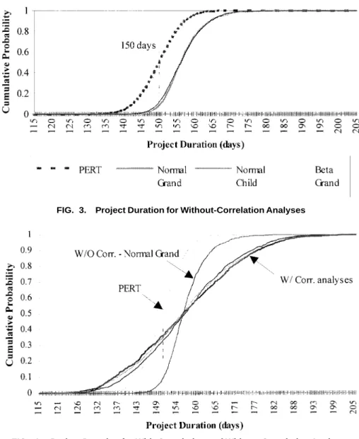
Cumulative duration distributions for the PERT and with-out-correlation simulations are presented in Fig. 3. The three without-correlation simulations show a project duration that is approximately 6.5 days (about 4%) greater than that generated by the PERT analysis. The distributions for the simulations are shifted to the right of the PERT distribution and have almost the same shape. This increase in project mean is due to the uncertainty associated with near-critical paths and is consistent with the observations of many other researchers (Crandall 1976; Moder et al. 1983). The three without-correlation

FIG. 3. Project Duration for Without-Correlation Analyses

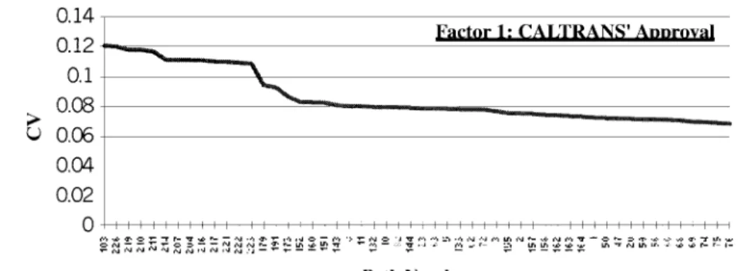
FIG. 4. Project Duration for With-Correlation and Without-Correlation Analyses

ulations produce similar results; there is not much difference between the assumption of a Normal Grand and Beta Grand. Therefore, for this example, NETCOR’s inability to capture a Beta Grand distribution for each activity is not significant.

The standard deviation for without-correlation simulations increases only slightly (about 2%) compared with PERT. In this project, the uncertainty associated with most near-critical paths is small and thus has little effect on the variability of the project’s duration. Finally, although the analyses have ilar values of standard deviation, the without-correlation sim-ulations result in a higher value of EDP and probability of schedule overrun compared with the PERT analysis, due to the rightward shift of the mean duration.

Normal Grand versus With-Correlation Analyses

Fig. 4 shows cumulative duration distributions for the PERT, Normal Grand, and with-correlation analyses (Scales 1 – 3). Correlation results in an increase in standard deviation for each path, so it is expected that the standard deviation of the project’s duration also will increase. However, the ex-pected project duration should not vary greatly with respect to the without-correlation simulations.

As expected, the without-correlation and with-correlation analyses show very little difference in expected project dura-tions. Correlation does increase a project’s standard deviation. Compared to without-correlation analysis, correlation caused an increase in the standard deviation of 9.56, 9.15, and 7.86

days (166, 159, and 136%) for Scales 1 – 3, respectively. These increases are significant at the 5% level [by a one-tailed sta-tistical test of the differences between means of a small sample size (Levin and Rubin 1991)].

Correlation also results in an increase of EDP of 41, 35, and 33% for Scales 1 – 3, respectively. If the daily liquidated damage of $2,200 (an amount that does not include overhead) is used as a daily delay penalty DP, the expected delay penalty is increased by $22,638 under Scale 1.

The range of 90% confidence intervals is increased from 19 to about 48 days. This again shows that correlation leads to the possibility of a much longer or much shorter project du-ration. The probability of schedule overrun depends upon what target date is set. In Fig. 4, the without-correlation and with-correlation distributions intersect with each other when a project’s duration is approximately 156.5 days. If the project completion date is set to 156.5 days, then both analyses have the same probability of schedule overrun, about 50%. If the target date is <156.5 days, then the without-correlation anal-yses will have a higher probability of overrun. On the other hand, if the target date is >156.5 days (to the right of the intersection date), then the with-correlation analyses will in-dicate a higher probability of schedule overrun. When the tar-get date is set to 150 days (i.e., CPM project duration), the probabilities of schedule overrun for without-correlation and with-correlation analyses are 91 and 64% (for Scale 1), re-spectively.

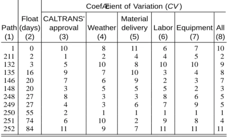
FIG. 5. Uncertainty Sensitivity due to CALTRANS’ Approval for 52 Paths TABLE 2. Average CV Values by Factor under Different Scale

Systems Scale (1) CAL-TRANS’ approval (2) Weather (3) Material delivery (4) Labor (5) Equipment (5) All factors (7) 1 0.088 (1) 0.018 (5) 0.035 (3) 0.038 (2) 0.028 (4) 0.107 2 0.070 (1) 0.017 (5) 0.029 (4) 0.051 (2) 0.047 (3) 0.106 3 0.068 (1) 0.021 (5) 0.024 (4) 0.046 (2) 0.037 (3) 0.098 Note: Number in parentheses represents the rank among five factors for each scale system.

With-Correlation Analyses under Different Scale Systems

For this example, the choice of a scale system has little effect on the results. This is true even in the case of Scale 3, which exaggerates the differences between high, medium, and low sensitivities. In general, Scale 1 shows the greatest cor-relation effect, as evidenced by its high values of standard deviation and EDP, whereas Scale 3 yields relatively smaller values in both categories. Scale 3 will be likely to exaggerate the correlation effect only when most activities have higher sensitivities to the same factor(s). Further discussion of scale systems and factor sensitivity can be found in Wang (1996).

Uncertainty Sensitivity along Path

Knowledge of the paths that show the greatest sensitivities to individual factors and combinations of factors can help sup-port project management. Although this project has only 227 activities, there are 2,773 paths through the project network. Further analysis of uncertainty sensitivity along a path was carried out on 252 paths (9%), with selection based on the following criteria:

• Select paths that may require management’s attention. Se-lection was based on float; for this case study, paths with float <20 days (<13% of project duration) were consid-ered.

• Select paths that may delay the progress of work follow-ing a ready-to-start activity. Paths selected under this cri-terion are those with minimum float (but perhaps >20 days) following a ready-to-start activity.

Based on these 252 paths, the following analyses are con-ducted:

• All paths were analyzed to examine the impact of differ-ent scale systems.

• Fifty-two paths that have float not exceeding 10 days were analyzed to compare the factor sensitivity of paths. • Eleven ready-to-start paths were analyzed to compare

fac-tor sensitivity for the minimum float paths that follow the 11 ready-do-start activities.

Analysis of 252 Paths

Table 2 summarizes the average values of CV for each factor under each scale system. Three observations are derived from Table 2. In this project, the project manager’s rank of the im-portance of factors (from most important to least important) was based on CALTRANS’ approval, weather, material deliv-ery, labor, and equipment. Under Scale 1, the five factors are ranked according to CV in the following order: CALTRANS’ approval, labor, material delivery, equipment, and weather. These results shows that a factor that is initially considered as more important by the project manager (such as weather) may not necessarily cause higher uncertainty sensitivity along a path. This is because the uncertainty sensitivity along a path for a factor also depends on the number of path activities that are sensitive to the factor and variance of factor-sensitive par-ent distributions.

Second, although Scale 1 ranks material delivery and equip-ment as the third and fourth factors affecting uncertainty along paths, under Scales 2 and 3, the rankings of these factors are reversed. In other words, the selection of a scale system can affect the results of uncertainty sensitivity along a path in this project.

Third, with the consideration of all five factors together, on average, Scale 3 results in a slightly smaller value of CV along a path. Exaggerating the difference between levels of influence does not necessarily highlight the correlation effect; con-versely, it may actually reduce the effect depending on the sensitivities of activities to the factors and on the configuration of child distributions. This is discussed in greater detail in Wang (1996).

Analysis of 52 Paths That Have Float Not Exceeding 10 Days

Fifty-two paths have float not exceeding 10 days. Fig. 5 shows the result of rankings by sensitivity due to F1. In the figure, it is found that Path 103 (path float = 7 days) is the most sensitive path with respect to CALTRANS’ approval. Re-sults of rankings by sensitivity due to F2 – F5 and all factors are included in Wang (1996). This information shows which factors are of concern on near-critical paths.

Analysis of 11 Ready-To-Start Paths

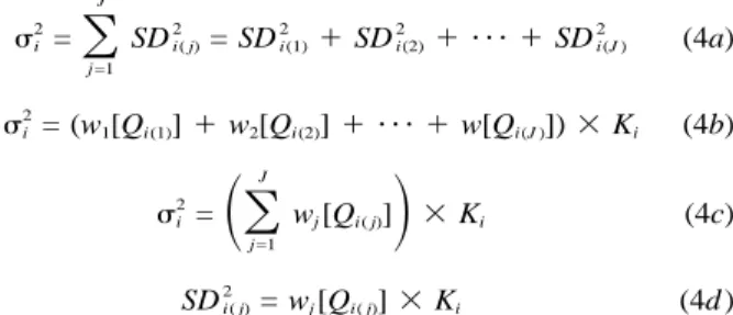
This analysis considers only the path that has the least amount of float among those following a ready-to-start activ-ity. Two types of results are presented here: sensitivities be-tween paths and sensitivities along each path. The results of sensitivities between paths are presented in Table 3. Path 250 is ranked as the path with highest sensitivity to factors other

TABLE 3. Rankings of Uncertainty Sensitivities for 11 Paths Path (1) Float (days) (2) Coefficient of Variation (CV ) CALTRANS’ approval (3) Weather (4) Material delivery (5) Labor (6) Equipment (7) All (8) 1 0 10 8 11 6 7 10 211 2 1 2 4 4 5 2 132 3 5 10 8 10 10 9 135 16 9 7 10 3 4 8 146 20 7 6 9 2 3 7 148 20 3 5 5 5 2 3 248 27 8 3 3 8 6 5 249 27 4 3 6 7 9 5 250 55 2 1 1 1 1 1 251 74 6 10 2 9 8 4 252 84 11 9 7 11 11 11

TABLE 4. Impact of Worse-than-Expected CALTRANS’ Ap-proval Project duration (1) Worse-than-expected analysis (2) Original analysisa (3) Difference (worse-than-expected analysis_⫺ original analysis) (4) Mean 170.88 156.51 14.37 Standard deviation 9.77 15.32 — EDP 21.32DP 10.29DP 11.03DP 90% confidence intervals 155–188 (⌬ = 33) 133–182 (⌬ = 49) — Probability of overrun 0.99 0.64 0.35

Note: EDP = expected delay penalty; DP = daily delay penalty.

a

Under Scale 1. than CALTRANS’ approval. However, the path has 55 days

of float and therefore may not require management’s imme-diate attention. Path 1 (critical path), Path 211 (2 days of float), and Path 132 (3 days of float) have <2 weeks of float. Among these three paths, path 211 has the highest sensitivities to each factor. The results of which factor has the greatest influence along a given path are included in Wang (1996).

Path Criticality

The introduction of correlation leads to increased variability in path duration. The factor sensitivity and float of near critical paths could be such that correlation has an impact on critical-ity. In the Presidio project, the maximum change in criticality occurs in path 1 (21% criticality without correlation versus 16% criticality with correlation). The average change in crit-icality is small (0.1%). Further discussion of critcrit-icality can be found in Wang (1996).

Information to Support Management Decisions

Based on the manager’s inputs, the outputs generated by NETCOR can support schedule uncertainty management in three ways:

Project Duration

Considering both uncertainty and correlation, NETCOR (under Scale 1) estimates that the project will be completed between 133 and 182 days with 90% confidence. The proba-bility that the project will be completed later than the CPM duration (150 days) is 64%. The expected delay penalty of the project is 10.29DP (where DP = daily delay penalty). If the daily liquidated damage is used as DP (i.e., $2,200), the EDP is $22,638.

Uncertainty Sensitivity along Path

On average, CALTRANS’ approval (F1) has the greatest impact on path duration, followed by labor (F4), material de-livery (F3), equipment (F5), and weather (F2). The project manager’s original ranking of importance was F1, F2, F3, F4, and F5. At the start of the project, most attention should be given to Path 1 (critical path), Path 211 (path float = 2 days), and Path 132 (path float = 3 days). Among these three paths, Path 211 has the highest sensitivity (i.e., highest CV value) to each factor and all factors combined. If conditions for a par-ticular factor are worse than expected, management should fo-cus attention on path 211 to mitigate the impact. In managing the uncertainty along Paths 211 and 132, F1 is most important, followed by F3, F4, F5, and F2. In managing the uncertainty along Path 1, F1 is most important, followed by F4, F5, F3, and F2.

Impact of CALTRANS’ Approval on Project Duration

For this project, owner-caused delays due to the time re-quired to obtain CALTRANS’ approval are of major concern to the contractor. NETCOR can be used to evaluate the pos-sible effect of delays in CALTRANS’ approval on a proj-ect’s duration. In this approach, the results for a NETCOR analysis in which CALTRANS’ approval is always worse-than-expected are compared with those of the original analysis. This shows the impact of a worse-than-expected response by CALTRANS.

First, the same inputs previously provided are used. Then, NETCOR is used to evaluate the project under the worse-than-expected condition for CALTRANS’ approval for each activ-ity. That is, the better-than-expected (left-hand-side) child and expected (central) child with respect to CALTRANS’ approval are removed. The simulation results are presented in Table 4. It is found that worse-than-expected CALTRANS’ approval results in an increase of about 14 days in expected project duration and about 11DP (where DP is daily delay penalty) in expected delay penalty. If the target date is set to be the CPM project duration (150 days), then the project has only a 1% chance to be completed by the target date under the worse-than-expected CALTRANS’ approval. The standard deviation is lower than in the original analysis due to reduced variance in the CALTRANS’ approval factor; for each activity, samples are drawn only from the worse-than-expected child distribu-tion rather than each of the three child distribudistribu-tions. As ex-pected, the range of 90% confidence intervals of the project’s duration is shifted to the right when the condition of CAL-TRANS’ approval is worse-than-expected for each act-ivity.

This type of ‘‘factor impact’’ analysis could be a useful planning tool if carried out at the start of the project. The owner and contractor would each be aware of the potential impact of poorer-than-expected conditions for each factor. Some of these factors may be under the contractor’s control (such as equipment), some may be under the owner’s control (such as CALTRANS’ approval in this example), and some may be under the control of neither party (such as weather). In all cases, an initial understanding of the impact of the factor condition on a project’s duration should help the owner and contractor work together to ensure that the project is com-pleted on time.

CONCLUSIONS AND FUTURE WORK

The case study described in this paper represents the first application of NETCOR to a full-scale construction project. The results are encouraging, in terms of both significance of

correlation and NETCOR’s ease of use. For the Presidio Vi-aduct seismic retrofit, analysis using NETCOR showed that the impact of correlation on the variability of the project’s duration is large enough to be of interest. In addition, NET-COR allowed an analysis of the importance of the factors af-fecting the project’s duration. For the Presidio project, the NETCOR analysis showed that, when the effects of the sched-ule network were considered, these factors had different rela-tive importance than the project manager had anticipated. The case study also demonstrated one of NETCOR’s most prom-ising applications, as a planning tool to investigate the im-pact of particular factor conditions. For a Presidio project, NETCOR was used to quantify the impact that worse-than-expected turnaround time for CALTRANS’ approval had on the project.

NETCOR’s use of qualitative estimates of the effect of fac-tor-based uncertainty allows correlation to be incorporated without excessive demands on the user. The project manager for the Presidio project found the required input (three-point duration estimates and factor sensitivities) to be reasonable. Although the NETCOR software is still a research prototype, it was easy to apply to the Presidio project.

The computer hardware used in this case study resulted in run times that, although acceptable for research, would be too long for the practical use of NETCOR in the field. Further work on NETCOR’s implementation, combined with the re-duced cost of faster computers, will allow faster run times.

Additional research needs are described in greater detail in Wang (1996). This paper has presented a single case study; many additional projects must be analyzed before general con-clusions can be drawn regarding the effects of correlation on a project’s duration.

ACKNOWLEDGMENTS

The writers thank the reviewers of this paper for their careful evalu-ation and thoughtful comments. The writers are grateful to John Bliss, the project manager who participated in this study. Without his interest and input, this application example would not have been possible.

APPENDIX. REFERENCES

Crandall, K. C. (1976). ‘‘Probabilistic time scheduling.’’ J. Constr. Div., ASCE, 102(3), 415–423.

Levin, R. I., and Rubin, D. S. (1991). Statistics for management, 5th Ed., Prentice-Hall, Englewood Cliffs, N.J.

Martinez, J. C. (1996). ‘‘STROBOSCOPE: State and resource based sim-ulation of construction processes.’’ PhD dissertation, University of Michigan, Ann Arbor, Mich.

Moder, J. J., Philips, C. R., and Davis, E. W. (1983). Project management with CPM, PERT and precedence diagramming, 3rd Ed., Van Nostrand Reinhold, New York.

Wang, W.-C. (1996). ‘‘Model for evaluating networks under correlated uncertainty—NETCOR.’’ PhD dissertation, University of California, Berkeley, Calif.

Wang, W.-C., and Demsetz, L. A. (2000). ‘‘Model for evaluating networks under correlated uncertainty—NETCOR.’’ J. Constr. Engrg. and Mgmt., ASCE, 126(6), 458–466.