Regression Analysis for Marginal Failure Probability
under Competing Risks
Wei-Hwa Chang
Weijing Wang
Email: wjwang@stat.nctu.edu.tw
Institute of Statistics, National Chiao-Tung University
Hsin-Chu, Taiwan, R.O.C.
December, 2006
Under Revision by Statistica Sinica
Abstract. The cumulative incidence function provides intuitive summary informa-tion about competing risks data. Via a mixture decomposiinforma-tion of this funcinforma-tion, we study covariate effects on the marginal probability of developing a particular cause of failure at a given time point without specifying the corresponding failure time distribution. Sev-eral inference methods are constructed based on two principles of handling missing data due to censoring, namely the imputation approach and the weighting approach. Our work extends part of the results in Fine (1999) and Wang (2003). Large sample prop-erties of the proposed estimators are derived and their finite sample performances are examined via simulations. For illustrative purposes, the proposed methods are applied to the well-known Heart Transplant data and is compared with the analysis of Larson and Dinse (1985) which was developed under the framework of a mixture model.
Key words : Cause-specific hazard; Mixture model; Imputation; Cumulative incidence
function; Inverse probability of censoring; Logistic regression; Missing Data.
1
Introduction
Multiple events data are commonly seen in biomedical studies. Under the framework of competing risks, subjects may fail from one of several different causes. Let T be the failure time and ˜B be the corresponding cause of failure taking values from the set {1, . . . , J}. Competing risks data naturally can be summarized by the following two
quantities. One is the cause-specific hazard function defined as
λj(t) = lim
∆t→0
Pr(T ∈ [t, t + ∆t), ˜B = j|T ≥ t)
∆t
which is the rate of occurrence for type-j failure in presence of all causes of failure. The other is the cumulative incidence function, or the crude failure probability, defined as
Fj(t) = Pr(T ≤ t, ˜B = j),
which describes the cumulative probability of developing type-j failure by time t. This paper considers regression analysis of Fj(t) which provides more direct information about
the cumulative risks and hence can be more easily explained to clinicians.
There is a functional relationship between the cause-specific hazard function and the cumulative incidence function such that
Fj(t) =
Z t
0
S(u−)λj(u)du,
and S(t) = Pr(T > t) = exp(−R0tPJj=1λj(u)du). Some authors including Cheng, Fine
and Wei (1998) have suggested to make inference of the cumulative incidence function by specifying regression models for all causes of hazards. However, since the effect of a covariate on λj(t) can be very different from its effect on Fj(t), the conclusion based
on such an indirect approach may be misleading. Also the parameters in the models for cause-specific hazards may lack simple interpretation in terms of the crude failure probabilities.
There have been growing interests in directly modelling the cumulative incidence function for a particular cause. Suppose that the first type of failure is of main inter-est. Fine and Gray (1999) and Fine (2001) both considered semi-parametric regression
models of the form,
g(F1(t|z)) = h(t) + zTθ, (1)
where z is a p × 1 vector of covariates, g(·) is a link function mapping from (0, 1) to (−∞, ∞) and h(t) is an unknown monotone function. Fine and Gray (1999) studied estimation in this model with the complementary log-log link function which leads to a proportional hazards assumption on the improper variable T1=T · I( ˜B = 1) + ∞ · I( ˜B 6=
1). Fine (2001) further extends this approach to more general transformation models which include the proportional odds model with the logistic link function.
Another popular analysis suggests a mixture model that expresses the cumulative incidence function as
Fj(t) = πj(1 − Qj(t)), (2)
for j = 1, . . . , J, where πj = Pr( ˜B = j) measures the marginal probability of type-j
fail-ure, and 1 − Qj(t) = Pr(T ≤ t| ˜B = j) describes the corresponding latency distribution
for the sub-population with ˜B = j. Wang (2003) considered nonparametric analysis
under a two-path framework which is a special case of model (2) with J = 2. In pres-ence of right censoring, Wang (2003) showed that valid estimators of πj and Qj(t), the
probability of experiencing path-j and the sojourn time for the path, can be obtained only if the follow-up period is long enough to recover the tail information of the first failure time. Specifically let C be the censoring variable. Define the two support points:
τT =sup{t: Pr(T > t) > 0} and τC =sup{t: Pr(C > t) > 0}. Wang (2003) mentioned
that πj and Qj(t) may not be identifiable if τT > τC.
For model (2) with covariates, Larson and Dinse (1985) assumed a multinomial logit model for πj and a parametric proportional hazard model for Qj(t), and suggested
the EM algorithm in the estimation procedure. Kuk (1992) considered a similar mix-ture model, in which the latency component follows a semi-parametric proportional hazard model, and took a rank likelihood approach in estimation. Notice that the maximum likelihood approach handles the estimation of πj and Qj(t) jointly so that
other component. Fine (1999) also considered a binary regression model for πj and a
semi-parametric transformation model for Qj(t). Instead of using the likelihood
ap-proach, he proposed two estimating functions for the two components in (2) separately. This approach is more robust compared with previous methods but faces the issue of non-identifiability if τT > τC. To remedy the potential problem, Fine (1999) modeled
πj(τ ) = Pr(T ≤ τ, ˜B = j) and Qj(t|τ ) = Pr(T > t|T ≤ τ, ˜B = j) instead, where τ is a
predetermined time point satisfying τ < τX, where τX = τC∧ τT.
In this article, we also study model (2) and focus on regression analysis of the marginal failure probability πj. The severe acute respiratory syndrome (SARS)
pro-vides an example. SARS is an epidemic and life-threatening acute disease that resulted in a global outbreak in 2003. A patient who was discharged from the hospital and was still alive at that time can be considered as being cured. Clinicians and the pubic usually are more interested in finding out which characteristics of a patient would affect his/her probability of being cured. We adopt a similar regression model as in Fine (1999) such that Fj(t ∧ τ |Z) can be written as
Pr(T ≤ τ, ˜B = j|Z)Pr(T ≤ t|T ≤ τ, ˜B = j, Z) = π(ZTβ(τ ))(1 − Qj,Z(t|τ )), (3)
where Z = [1, zT]T is the (p + 1) × 1 covariates, π(·) is a known function mapping from
(−∞, ∞) to (0, 1), β(τ ) is a (p + 1) × 1 vector of parameters and τ satisfies τ < τX
to avoid the problem of non-identifiability. Notice that we do not specify the form of
Qj,Z(t|τ ) since our primary concern is the marginal failure probability πj(τ ). In Section
2, we apply two principles of handling missing data to estimate β(τ ). The first approach utilizes the technique of weighting to adjust for the censoring bias which has also been considered by Fine (1999). The proposed estimator of of β(τ ) is more efficient than Fine’s estimator. The second proposal uses the technique of imputation which extends the idea of Wang (2003) from a nonparametric setting to the regression framework. Technical results are summarized in the appendix. Section 3 contains simulation studies and data analysis. In Section 4, we give some concluding remarks.
2
The Proposed Methods
2.1
Preliminary
Without loss of generality, consider only two causes of failures, namely ˜B = j (j = 1, 2).
Denote {(Ti, ˜Bi, Zi) (i = 1, . . . , n)} as a random sample of (T, ˜B, Z) under model (3).
To simplify the notation, we will write β = β(τ ) for model (3). The likelihood function of β is given by ˜ L(β) = n Y i=1 © π(ZT i β) ª∆1i {¯π(ZT i β)}1−∆1i, (4)
where ∆1i= I( ˜Bi = 1, Ti ≤ τ ) and ¯π(t) = 1−π(t). The resulting score function becomes
˜ U(β) = n X i=1 © ∆1i− π(ZTi β) ª πφ(ZTi β) π(ZT i β)¯π(ZTi β) Zi, (5) where πφ(t) = ∂π(t)/∂t.
In presence of right censoring, the value of ∆1imay be unknown. Observed variables
become {(Xi, Bi, Zi) (i = 1, . . . , n)}, which are iid replications of (X, B, Z) where X =
T ∧ C and B = ˜B · I(T ≤ C). Under censoring, the likelihood function of β becomes
very complicated and involves specification of several nuisance functions such as Pr(T >
t| ˜B = j, T ≤ τ, Z) and Pr(T > t| ˜B = j, T > τ, Z) for j = 1, 2. We propose to directly
modify the score function ˜U(β) by applying two useful principles of handling missing
data, namely the weighting approach and the imputation approach. We assume that, given Z, C is independent of (T, ˜B) and, to simplify the analysis, T and C are both
continuous variables.
2.2
Inverse Probability Weighting
To simplify the notations, let δ1i = I(Bi = 1), δ2i = I(Bi = 2) and δi = δ1i+δ2i. Suppose
that the censoring distribution depends on Z only through some discrete covariates L which means that Pr(C ≥ t|Z) = Pr(C ≥ t|L) = GL(t). The observable response
I(X ≤ τ, δ1 = 1) can be treated as a biased proxy of ∆1. Moreover E µ I(X ≤ τ, δ1 = 1) GL(X) ¯ ¯ ¯ ¯ Z ¶ = E · I(T ≤ τ, ˜B = 1)E µ I(T ≤ C) GL(T ) ¯ ¯ ¯ ¯ T,B, Z˜ ¶¯¯ ¯ ¯ Z ¸ = E (∆1| Z) = π(ZTβ), (6)
which means that by taking an inverse weighting adjustment of I(X ≤ τ, δ1 = 1), we
can obtain an unbiased proxy of ∆1. Replacing ∆1i by I(Xi ≤ τ, δ1i = 1)/ ˆGLi(Xi) in
the score function (5), Fine (1999) proposed the following estimating function
UF(β) = n X i=1 ( I(Xi ≤ τ, δ1i = 1) ˆ GLi(Xi) − π(ZT i β) ) πφ(ZTi β) π(ZT i β)¯π(ZTi β) Zi, (7)
where ˆGL(t) is the Kaplan-Meier estimator of GL(t) with
ˆ GL(t) = Y u<t ½ 1 − Pn k=1PI(Xk = u, δk = 0, Lk = L) n k=1I(Xk ≥ u, Lk = L) ¾ . (8)
Although the estimating function UF(β) has an intuitive and simple form, it may not
be efficient since only a subset of the sample, (X, δ1), was used in its construction.
As a comparison with (6), it can be shown that
E · I(X > τ ) GL(τ +) + I(X ≤ τ, δ2 = 1) GL(X) ¯ ¯ ¯ ¯ Z ¸ = 1 − π(ZTβ) = ¯π(ZTβ), (9)
where GL(τ +) = Pr(C > τ |L). Equation (9) alone can be used to construct an
estimat-ing function of β as (7). However possible more efficient estimation can be achieved by incorporating equations (6) and (9). Specifically for i = 1, . . . , n, let
h1i = I(Xi ≤ τ, δ1i= 1) GLi(Xi) − π(ZT i β), h2i= I(Xi > τ ) GLi(τ +) + I(Xi ≤ τ, δ2i = 1) GLi(Xi) − ¯π(ZT iβ),
and hi = [h1i, h2i]T. Applying the principles discussed in Heyde (1997, Chap.2), the
optimal estimating function of β based on H = [hT
1, . . . , hTn]T is U∗(β) = −E µ ∂HT ∂β ¶ Σ−1H H = n X i=1 · −E µ ∂hT i ∂β ¶¸ Σ−1hi hi, (10) where ΣH = E(HHT), Σhi = E(hih T i ) = · v1i −π(ZTiβ)¯π(ZTi β) v2i ¸ and vji = V ar(hji) (j = 1, 2).
Because analytic expressions of v1i and v2i are not available, they can be replaced by
other related quantities. Specifically
v1i = E µ I(Xi ≤ τ, δ1i= 1) G2 Li(Xi) ¯ ¯ ¯ ¯ Zi ¶ − π2(ZT i β). (11)
Based on the first-order Taylor expansion, the first term of the variance (11) can be approximated by E µ 1 GLi(Xi) ¯ ¯ ¯ ¯ Zi ¶ E µ I(Xi ≤ τ, δ1i = 1) GLi(Xi) ¯ ¯ ¯ ¯ Zi ¶ = E µ 1 GLi(Xi) ¯ ¯ ¯ ¯ Li ¶ π(ZTiβ).
Although E (1/GL(X)| L) can be estimated by its moment estimate, this quantity is
too sensitive to the tail behavior of ˆGL. We suggest to use a related but more robust
quantity instead such as the sample median of {1/ ˆGLi(Xi) : Li = L, i = 1, . . . , n},
denoted as ML. Accordingly a reasonable proxy of v1i is ˆv1i = π(ZTi β)(MLi− π(Z
T i β)),
and by the same argument, we have ˆv2i = ¯π(ZTi β)(MLi − ¯π(ZTi β)). Using ˆv1i, ˆv2i and
ˆ
GLi(t) in replacement of the corresponding quantities in (10), the resulting estimating
function becomes U1(β) = n X i=1 h (ˆv2i− v3i)ˆh1i− (ˆv1i− v3i)ˆh2i i πφ(ZTi β) ˆ v1ivˆ2i− v23i Zi, (12) where ˆh1i= I(Xi ≤ τ, δ1i= 1) ˆ GLi(Xi) − π(ZT i β), ˆh2i= I(Xi > τ ) ˆ GLi(τ +) + I(Xi ≤ τ, δ2i = 1) ˆ GLi(Xi) − ¯π(ZT iβ),
and v3i = π(ZTi β)¯π(ZTi β). Since the estimating function U1(β) is motivated by the
idea of constructing the optimal estimating function, hopefully it is more efficient than
UF(β) which only utilizes partial data. Finite sample comparison will be evaluated via
simulations. Let β0 be the true value of β. The solution to U1(β) = 0 is denoted as
ˆ
β1. In Appendix A and B, we prove asymptotic normality of U1(β0) and ˆβ1. An iid
expression of n1/2(ˆβ
1 − β0) is given in (A.4) which will be used in variance estimation
described in Appendix B.
If C depends on continuous covariates L, ˆGL(t) can be estimated by the
nonpara-metric smoothing techniques summarized in Section 2.3. Sometimes to avoid the curse of dimensionality, one may impose parametric or a semi-parametric models to describe the covariate effect on C.
2.3
Imputation by Conditional Mean
Alternatively one can impute ∆1i by an estimate of its conditional mean given the data.
Specifically E(∆1i|Xi, δ1i, δ2i, Zi) equals
I(Xi ≤ τ, δ1i= 1) + I(Xi ≤ τ, δi = 0)pZi(Xi), (13)
where pz(x) = E(∆1i|δi = 0, Xi = x; Zi = z). The first proposed estimator of pz(x)
is derived under a purely nonparametric setting which generalizes the nonparametric results in Wang (2003) and Satten and Datta (2001). Their ideas are roughly summarized in Appendix C. With covariates, it follows that
pz(x) = Pr(T ≤ τ, ˜B = 1|T > x, Z = z) =
Pr(x < T ≤ τ, ˜B = 1|Z = z) Sz(x)
, (14) where Sz(t) = Pr(T > t|Z = z). When Z takes discrete values only, we can partition
the sample into several subsets according to the covariate values and then obtain ˆ Sz(t) = Y u≤t ½ 1 − Pn i=1PI(Xi = u, δi = 1, Zi = z) n i=1I(Xi ≥ u, Zi = z) ¾ . (15)
Accordingly a model-free estimator of pz(x), denoted by ˆpz(x), is given by
ˆ pz(x) = 1 ˆ Sz(x) Pn i=1I(x < XiP≤ τ, δ1i= 1, Zi = z)/ ˆGLi(Xi) n i=1I(Zi = z) . (16) where ˆGLi is obtained in (8).
For continuous Z, nonparametric estimators of Pr(x < T ≤ τ, ˜B = 1|Z = z) and Sz(x) can be derived using smoothing techniques. By applying the techniques of
non-parametric regression as illustrated in Dabrowska (1987), the formula of ˆpz(x) becomes
ˆ pz(x) = 1 Pn i=1 h I(Xi>x,δi=1) ˆ GLi(Xi) + I(Xi>X(m)) ˆ GLi(X(m)+) i Bn,i(z) n X i=1 I(x < Xi ≤ τ, δ1i= 1) ˆ GLi(Xi) Bn,i(z), (17) where X(m) is the largest observed failure time and Bn,i(z) is a random set of
non-negative weights. Candidates of the weight function include kernel type weights, nearest neighbors or local linear weights. For example one can use the kernel type weight
Bn,i(z) = K(a−1 n (z − Zi)) Pn j=1K(a−1n (z − Zj)) , (18)
where K(·) is an appropriate kernel function and an is a sequence of bandwidth.
Based on (13) one can construct the following estimating function
U2(β) = n X i=1 n ˆ ∆1i− π(ZTiβ) o π φ(ZTiβ) π(ZT i β)¯π(ZTi β) Zi, (19)
where ˆ∆1i = I(Xi ≤ τ, δ1i = 1) + I(Xi ≤ τ, δi = 0)ˆpZi(Xi) and ˆpZi(Xi) is given in (16)
or (17) depending on the type of Z.
The second proposal of estimating pz(x) utilizes the model assumption (3) in which
(14) can be further expressed as pz(x; β, Q1,z(·|τ ), Q2,z(·|τ ), Sz(τ )) which equals
Q1,z(x|τ )π(zTβ) Q1,z(x|τ )π(zTβ) + Q2,z(x|τ ){1 − Sz(τ ) − π(zTβ)} + Sz(τ ) . (20) We can estimate Sz(τ ) by Y u≤τ ½ 1 − Pn
i=1PI(Xi = u, δi = 1)Bn,i(z) n
i=1I(Xi ≥ u)Bn,i(z)
¾ , (21) and Qj,z(t|τ ) (j = 1, 2) by Y u≤t ½ 1 − Pn
i=1I(u = Xi ≤ τ, δji = 1)Bn,i(z)
Pn
i=1[I(u ≤ Xi ≤ τ, δji = 1) + I(u ≤ Xi ≤ τ, δi = 0)wj,Zi(Xi)] Bn,i(z)
¾
, (22)
where w1,z(x) is ˆpz(x) given in (16) or (17) depending on the type of Z and w2,z(x) is
obtained by replacing δ1 in ˆpz(x) with δ2. For continuous covariates, the weight function Bn,i(z) is given in (18) and for discrete covariates Bn,i(z) = I(Zi = z). By plugging
in appropriate estimators of Sz(τ ) and Qj,z(t|τ ) (j = 1, 2) in (20), the second proposed
estimating function based on (13) is given by
U3(β) = n X i=1 n ˜ ∆1i− π(ZTiβ) o π φ(ZTiβ) π(ZT i β)¯π(ZTi β) Zi, (23)
where ˜∆1i = I(Xi ≤ τ, δ1i = 1)+I(Xi ≤ τ, δi = 0)pZi(Xi; β, ˆQ1,Zi(·|τ ), ˆQ2,Zi(·|τ ), ˆSZi(τ )),
and ˆSZi(τ ) and ˆQj,Zi(·|τ ) (j = 1, 2) are given in (21) and (22).
The solution to Uj(β) = 0 is denoted as ˆβj (j = 2, 3). The two estimating functions
using the model information, we expect that it may perform better than U2(β). Their
finite-sample performances will be compared via simulations. Since U3(β) is a more
complicated function of β than U2(β), numerical computation of ˆβ3 becomes more
difficult. To simplify the root-finding procedure, one may treat ˜∆1ias a fixed number in
the mth iteration by using pz(x; ˆβ
(m−1)
, ˆQ1,z(·|τ ), ˆQ2,z(·|τ ), ˆSz(τ )) instead, where ˆβ
(m−1)
is the solution in the previous step. The final solution is obtained via an iterative procedure with m = 1, 2, . . .. The modified estimating function is a simpler function of
β and thus convergence can be achieved by only few steps of iterations.
When Z is discrete, we prove asymptotic normality of n−1/2U
2(β0) and that of n1/2(ˆβ
2 − β0) in Appendix D. Similar arguments can be applied to establish
asymp-totic properties of U3(β0) and ˆβ3. When there are continuous covariates, the imputed
estimators ˆpz(x) and ˆQj,z(x) involve a smoothing weight function Bn,i(z), which makes
the analytic analysis more complicated. Since this technical issue is not our main focus, we suggest to apply the bootstrap re-sampling technique to approximate the distribu-tions of Uj(β0) and ˆβj (j = 2, 3) for further inference. Its empirical performance is also
examined in our simulations and data analysis.
3
Numerical Analysis
3.1
Simulation Studies
Finite sample performances of the proposed estimators were assessed via simulations. The covariate Z was generated from three distributions. For the discrete case, Z was generated from a Bernoulli random variable with Pr(Z = 0) = Pr(Z = 1) = 1/2. For the continuous case, Z was generated from Normal(0, 1) or Unif(−3, 3). Given Z, we generated ∆1 = I(T ≤ τ, ˜B = 1) and ∆2 = I(T ≤ τ, ˜B = 2) as follows. First ∆1 was
generated from a Bernoulli distribution with mean π(β0+ β1Z), where π(β0+ β1Z) =
exp(β0+ β1Z)
1 + exp(β0+ β1Z) .
If ∆1 = 1, set ∆2 = 0 and, if ∆1 = 0, then generate ∆2 from a Bernoulli distribution
with mean π(α0+ α1Z). The parameters of interest are β0 and β1. Given (∆1, ∆2), the
failure time T was generated from a distribution with the density function fT which can
be expressed as fT(t) = f1(t|τ, Z) if (∆1, ∆2) = (1, 0) f2(t|τ, Z) if (∆1, ∆2) = (0, 1) f3(t|τ, Z) if (∆1, ∆2) = (0, 0),
where fj(t|τ, Z) (j = 1, 2) are density functions with supports no greater than τ and
f3(t|τ, Z) is a density function whose value exceeds τ . In the simulations, we set
fj(t|τ, Z) = fYj(t) 1 − SYj(τ ) I(t ≤ τ ) (j = 1, 2) and f3(t|τ, Z) = fY3(t) SY3(τ ) I(t > τ ),
where fYj(t) and SYj(t) is the density function and the survival function of Yj which
follows the accelerated failure-time model of the form
ln Yj = γ0,j + γ1,jZ + σj· Wj, (24)
where γ0,j, γ1,j and σj are (nuisance) parameters and Wj is the error distribution. The
censoring variable was generated from Unif(c0, c0+ c1), where c0 is pre-specified and the
value of c1 is determined to achieve the targeted censoring proportion (i.e. 30% or 40%).
After generating a random sample of (∆1, ∆2, T, Z, C), denoted as {(∆1i, ∆2i, Ti, Zi, Ci)
(i = 1, . . . , n)}, the observed data is {(Xi, δ1i, δ2i, Zi) (i = 1, . . . , n)}, where Xi = Ti∧Ci,
δ1i= ∆1iI(Ti ≤ Ci) and δ2i = ∆2iI(Ti ≤ Ci). The value of τ is set to be 2.5. The sample
size n was set to be 100 or 300.
Four estimators of β = (β0, β1)T were under evaluation. Besides the three proposed
estimators ˆβj (j = 1, 2, 3), for comparison, we also evaluated the estimator proposed by Fine (1999), denote it by ˆβF which solves UF(β) = 0. The criteria of comparison
include the average bias (BS), the sample standard deviation (SD), the mean squared errors (MSE) and the relative efficiency (RE) which is defined as the ratio of the mean square errors of ˆβF to that of ˆβj (j = 1, 2, 3).
Tables 1, 2 and 3 list the results for three types of the covariate Z respectively. For illustration, only the results for the estimator of β1 are presented; the results for the
estimator of β0 are similar and hence omitted. The proposed estimators ˆβj (j = 1, 2, 3)
are more efficient than ˆβF especially in the case of continuous covariate. Furthermore, ˆ
β2 and ˆβ3, obtained based on the imputation approach, perform better than ˆβ1 and ˆβF
which utilize the weighting approach. The estimator ˆβ3 with model-based imputation slightly performs better than ˆβ2 obtained by nonparametric imputation. The standard deviation estimates of ˆβ1 and ˆβF were computed using the formula given in (A.4) for three types of Z.
The standard deviation estimate of ˆβ2 can also be obtained by applying the formula (A.4) if Z is discrete but becomes intractable analytically if Z is continuous. The same problem occurs to standard deviation estimation of ˆβ3. In such a situation, we used the bootstrap re-sampling method. Specifically 1000 sub-samples were drawn with replacement from the original sample, and for ith sub-sample, we get ˆβ(i)k by solving
Uk(β) = 0 (k = 2, 3). Then the standard deviation estimate of ˆβk can be obtained
as the sample standard deviation of ˆβ(i)k (i = 1, . . . , 1000). In Tables 1 ∼ 3, we listed the average of the proposed standard deviation estimates (ASD) and the corresponding empirical coverage probabilities of nominal 95% confidence intervals for β (CP). For all the cases, the empirical coverage probabilities are close to the nominal level and the values of ASD are close to those of SD, the sample standard deviation.
In Table 4, we investigated the situation when C actually depends on Z such that ln C = γ0,c + γ1,cZ + σcWc. For the case of discrete Z, the data generation scheme is
same as that described for Table 1 and, for the case of continuous Z, the setup is same as in Table 2. In computation of the proposed estimators, we evaluated two estimators of G(t) = Pr(C ≥ t). One is the Kaplan-Meier estimator and the other is a kernel-type estimator which simply replaces δi = 1 by δi = 0 in formula (21). Note that the former
is based on the wrong assumption that C does not depend on Z. It turns out that the results based on the Kaplan-Meier estimator of G(t) are biased while the kernel approach yields less biased estimators. Generally speaking, it seems that the misspecification of
ˆ
G(t) has more influence on the bias term (BS) and less on the standard deviation (SD).
mis-specification.
3.2
Data Analysis
The proposed inference procedures are applied to the Stanford Heart Transplant data (Crowley and Hu, 1977, p. 28-29). The main objective is to explore the relationship between certain covariates and the cause of death due to transplant rejection. This dataset was analyzed by Larson and Dinse (1985) in the context of a mixture model. Deaths were attributed to transplant rejection ( ˜B = 1) or other causes ( ˜B = 2). Among
the 65 heart recipients, there were 29 rejected death (B = 1); 12 deaths were from other causes (B = 2) and 24 patients were censored (B = 0). The covariates include the waiting time from acceptance to surgery (w); the age at surgery (age) and a continuous mismatch score (m). Both m and age are transformed to have zero mean and unit variance, and w was recorded as a binary variable according to whether or not the waiting time exceeded 31 days. The survival time T (in days) was measured from the date of transplant surgery.
To determine if the censoring time C is related to the covariates, a Cox proportional hazard model was fitted for the censoring time C on each covariate respectively. Since that all p-values are greater than 0.1, the result indicates that all covariates have no significant effects on C. Hence we assume the independence between C and Z. Let
π(τ ) = Pr(T ≤ τ, ˜B = 1). We first investigated the marginal effect of each covariate for
four selected values of τ = 250, 500, 900, 1800. Under the logistic model log µ π(τ ) 1 − π(τ ) ¶ = b0(τ ) + b1(τ )Z,
all proposed methods show that the effect of waiting time w is not significant and hence can be removed. For other covariates, age is significant for all values of τ and the effect of the mismatch score m is insignificant for small values of τ and then becomes more obvious as τ increases. We further consider multiple logistic regression by including age and m jointly in the model. In Table 5 we see that age still plays an important role for all values of τ ; on the other hand the effect of mismatch score can be neglected when it
is considered jointly with age. Thus we conclude that age is the determining factor of
π(τ ), that is, a patient with younger age at transplant surgery will have a lower chance
to develop transplant rejection by time τ .
Larson and Dinse (1985) investigated the same dataset by setting τ = τT. It was
assumed that the incidence rate of transplant rejection, Pr( ˜B = 1), follows a logistic
model and the latency distribution 1 − Qj(t) = Pr(T ≤ t| ˜B = j) follows a proportional
hazard model with
Pr(T > t| ˜B = j, Z) = exp
·
−
Z t
0
hj(u) exp(ZTγj)du
¸
(25) where hj(t) is specified as a piece-wise exponential function for j = 1, 2. Their analysis
showed that no covariates have significant effect on Pr( ˜B = 1) but both age and m were
important for the latency distribution associated with transplant rejection. Specifically, for patients destined to die from transplant rejection, one with younger age at transplant surgery and with better tissue match would have better survival prognosis.
Although our analysis took τ < τT, Table 5 shows that the effect of age on π(τ )
persists throughout all selected values of τ . It is reasonable to expect that the effect of
age will continue to π(τT) = Pr( ˜B = 1) as τ approaches to τT. From this aspect, we
thought that the age at surgery plays an important role on a patient’s chance of dying from transplant rejection. Our conclusion conflicts with that of Larson and Dinse (1985) which contributes the age effect only to the latency distribution 1 − Q1(t).
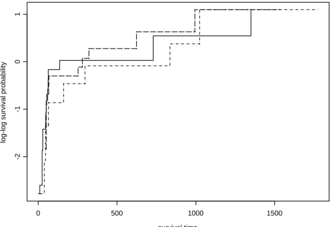
To clarify the contradiction between the two analyses, we checked whether the age effect on the hazard of T | ˜B = 1 is proportional. We partitioned the sample to three
groups with age ≤ 45 (group 1), 45 < age ≤ 51 (group 2) and 51 < age (group 3). Let ˆ
Q1,j(t) denote the estimator of Q1(t) for group j, where ˆQ1,j(t) (j = 1, 2, 3) were
calcu-lated using the formula proposed by Wang (2003) described in Appendix C. Under the proportional hazard assumption, plots of ln(− ln( ˆQ1,j)) should be approximately parallel
for j = 1, 2, 3. From Figure 1, we found that the curves are close to parallel for j = 1, 2. However ln(− ln( ˆQ1,3)) intersects with ln(− ln( ˆQ1,2)) first and then crosses ln(− ln( ˆQ1,1))
for age on Q1may not be adequate. Since Larson and Dinse (1985) adopted a parametric
approach by estimating the incidence rates and latency distributions jointly, we doubt that, if the assumption on the latency part is not accurate, the corresponding result for Pr( ˜B = 1) may not be valid. To confirm the above conjecture, we divided the data into
two groups with age≤ 45 and age> 45 and the results are similar.
4
Concluding Remarks
The proposed methods can be directly compared with the result of Fine (1999) in which the weighting approach is used to estimate the regression parameters for the marginal probability of a particular cause of failure. Here we consider two methods, namely im-putation and weighting. For the weighting approach, we also make concrete suggestions to improve efficiency. The imputation approach tends to work better in simulations but the corresponding analytic derivations are more complicated and may involve smooth-ing techniques if the covariate is continuous. The two inference techniques are popular in handling missing information and have been used by Jung (1996) and Subramanian (2001) in estimating the long term survival rate without competing risks.
Comparing our model (3) with the model (1) studied in Fine and Gray (1999) and Fine (2001), we find that setting t = τ and g−1(x) = π(x), model (1) coincides with
model (3) and β(τ ) = [h(τ ), θT]T. In other words, model (3) fits the data at a single time point τ while model (1) considers the entire time span. If model (1) is appropriate, then the last p components of β(τ ) derived from model (3) will be similar for different choices of τ . Therefore results obtained for model (3) provides a way to verify the assumption of model (1) or help choosing time-dependent covariates in that model. Formally the assumption of model (1) can be verified by testing H0 : ˜β0(τ1) = ˜β0(τ2) for any τ1 6= τ2,
time τ . Specifically let R = 0 1 0 . . . 0 0 0 1 . . . 0 ... ... ... ... ... 0 0 0 . . . 1 p×(p+1) . Under H0, n1/2R · n ˆ β1(τ2) − ˆβ1(τ1) o can be approximated by n−1/2R ·©A−11 (ZTβ0(τ2)) · U1(β0(τ2)) − A−11 (ZTβ0(τ1)) · U1(β0(τ1)) ª
which converges to a mean-zero p dimensional normal random variable. The analytic expression of the above function given in (A.4) can be used in performing the test.
Appendix
Appendix A: Asymptotic properties of U1(β)
Recall the notations defined for the estimating function U1(β) in Section 2.2, we have U1(β) = n X i=1 [(ˆv2i− v3i)h1i− (ˆv1i− v3i)h2i] πφ(ZTi β) ˆ v1ivˆ2i− v3i2 Zi+ B2n(β), where B2n(β) = n X i=1 (· I(Xi ≤ τ, δ1i = 1) GLi(Xi) ˆ v2i− v3i ˆ v1iˆv2i− v3i2 πφ(ZTiβ)Zi ¸ GLi(Xi) − ˆGLi(Xi) ˆ GLi(Xi) − · I(Xi ≤ τ, δ2i= 1) GLi(Xi) ˆ v1i− v3i ˆ v1ivˆ2i− v3i2 πφ(ZTi β)Zi ¸ GLi(Xi) − ˆGLi(Xi) ˆ GLi(Xi) − · I(Xi > τ ) GLi(τ +) ˆ v1i− v3i ˆ v1ivˆ2i− v23i πφ(ZTi β)Zi ¸ GLi(τ +) − ˆGLi(τ +) ˆ GLi(τ +) ) .
Suppose that the true value β0is located in the interior of the parameter space, which is a bounded convex region and πφ(·) is bounded. To derive the asymptotic distribution
of n−1/2U
1(β0), we first express the Kaplan-Meier estimator ˆGL(t) in the integral form,
GL(t) − ˆGL(t) GL(t) = n X i=1 Z t 0 ˆ GL(u−) GL(u)
I(Li = L)dMC,i(u)
¯
YL(u)
where
MC,i(u) = I(Xi ≤ u, δi = 0) −
Z u 0 I(Xi ≥ s)dΛC,Li(s), ¯ YL(u) = Pn
i=1I(Xi ≥ u, Li = L) and ΛC,L(s) is the cumulative hazard function of
C given L. By the uniform convergence of the Kaplan-Meier estimator, we can write n−1/2B 2n(β0) as 1 √ n n X i=1 Z ∞ 0 [q1,Li(t; β0) − q2,Li(t; β0) − q3,Li(t; β0)] µ ¯YLi(t) n ¶−1 dMC,i(t) + op(1), where q1,Li(t; β0) = 1 n n X k=1 I(Xk ≥ t, Lk = Li) · I(Xk ≤ τ, δ1k = 1) GLk(Xk) ¸ v2k− v3k v1kv2k− v23k πφ(ZTkβ0)Zk, (A.1) q2,Li(t; β0) = 1 n n X k=1 I(Xk ≥ t, Lk = Li) · I(Xk ≤ τ, δ2k = 1) GLk(Xk) ¸ v1k− v3k v1kv2k− v23k πφ(ZTkβ0)Zk, (A.2) q3,Li(t; β0) = 1 n n X k=1 I(τ ≥ t, Lk = Li) · I(Xk > τ ) GLk(τ +) ¸ v1k− v3k v1kv2k− v23k πφ(ZTkβ0)Zk, (A.3) v1k = π(ZTkβ0)( ˜MLk−π(Z T kβ0)), v2k = ¯π(ZkTβ0)( ˜MLk−¯π(Z T kβ0)), v3k = ¯π(ZkTβ0)π(ZTkβ0)
and ˜ML is the median of the random variable 1/GL(X).
Therefore n−1/2U1(β 0) can be expressed as n−1/2 Pn i=1ξi+ op(1), where ξi = ½· I(Xi ≤ τ, δ1i = 1) GLi(Xi) − π(ZT i β0) ¸ (v2i− v3i) − · I(Xi > τ ) GLi(τ +) + I(Xi ≤ τ, δ2i = 1) GLi(Xi) − ¯π(ZTi β0) ¸ (v1i− v3i) ¾ πφ(ZTi β0) v1iv2i− v23i Zi + Z ∞ 0 qLi(t; β0) yLi(t) dMC,i(t),
yLi(t) = limn→∞Y¯Li(t)/n and qLi(t; β0) = limn→∞[q1,Li(t; β0) − q2,Li(t; β0) − q3,Li(t; β0)].
Since {ξi (i = 1, ..., n)} are zero-mean independent random variables, by the multivariate
central limit theorem, n−1/2U
1(β0) has an asymptotic normal distribution with mean 0
and covariance matrix Γ1 = limn→∞n−1
Pn
Appendix B: Asymptotic properties of ˆβ1
Let ˆβ1 be the solution to U1(β) = 0. Since U1(β) is differentiable with respect to β and has a bounded derivative, consistency of ˆβ1 follows. By a Taylor expansion of
n−1/2U
1(β) with respect to β0, we can write
0 = n−1/2U1(ˆβ1) = n−1/2U1(β0) − A1(β0) n1/2(ˆβ1− β0) + op(1), where A1(β0) = − limn→∞ 1 n ∂U1(β) ∂βT ¯ ¯ ¯ ¯ β=β0 . It follows that n1/2(ˆβ1− β0) = [A1(β0)]−1n−1/2U1(β0) + op(1). (A.4) Hence n1/2(ˆβ
1− β0) has an asymptotically normal distribution with mean 0 and
covari-ance matrix V1 = [A1(β0)]−1Γ1[A1(β0)]−1.
Replacing β0, GL, yL(t) and dΛC,L(t) with ˆβ1, ˆGL, ¯YL(t)/n and dNC,L(t)/ ¯YL(t),
where NC,L(t) =
P
kI(Xk≤ t, δk = 0, Lk = L), respectively, ˆξi equals
(" I(Xi ≤ τ, δ1i= 1) ˆ GLi(Xi) − π(ZT i βˆ1) # (ˆv2i− ˆv3i) − " I(Xi > τ ) ˆ GLi(τ +) +I(Xi ≤ τ, δ2i = 1) ˆ GLi(Xi) − ¯π(ZT i βˆ1) # (ˆv1i− ˆv3i) ) πφ(ZTi βˆ1) ˆv1iˆv2i− ˆv23i Zi +PnI(δi = 0)ˆqLi(Xi; ˆβ1) n k=1I(Xk ≥ Xi, Lk = Li) − n X j=1 nI(δj = 0, Xi ≥ Xj, Lj = Li)ˆqLi(Xj; ˆβ1) (Pnk=1I(Xk ≥ Xj, Lk = Li))2 , where ˆv1i = π(ZTi βˆ1)(MLi−π(ZiTβˆ1)), ˆv2i= ¯π(ZTi βˆ1)(MLi−¯π(ZTi βˆ1)), ˆv3i= ¯π(ZTi βˆ1)π(ZTi βˆ1), ˆ qLi(t; ˆβ1) = ˆq1,Li(t; ˆβ1) − ˆq2,Li(t; ˆβ1) − ˆq3,Li(t; ˆβ1),
and ˆqj,Li(t; ˆβ1) (j = 1, 2, 3) are obtained by using ˆβ1, ˆGLk and (ˆv1k, ˆv2k, ˆv3k) instead of
β0, GLk and (v1k, v2k, v3k) in (A.1)−(A.3). It follows that the covariance matrix Γ1 can
be estimated by ˆΓ1 = n−1 Pn i=1ξˆiξˆi T and then ˆ V1 = h ˆ A1(ˆβ1) i−1 ˆ Γ1 h ˆ A1(ˆβ1) i−1 where ˆ A1(ˆβ1) = n X i=1 1 n · ˆv1i+ ˆv2i− 2ˆv3i ˆv1iˆv2i− ˆv3i2 π2φ(ZTi βˆ1)ZiZTi ¸ .
Appendix C: Previous nonparametric results of Wang (2003)
Wang (2003) estimated the conditional path probability given T > x. Modifying her idea, we can estimate pj(x) = Pr(T ≤ τ, ˜B = j|T > x) by
ˆ pj(x) = 1 n ˆS(x) n X i=1 I(x < Xi ≤ τ, δji = 1) ˆ G(Xi) ,
where ˆS(x) is the Kaplan-Meier estimator of S(x) which, according to (Satten and Datta,
2001), can be re-expressed as an average of inverse probability of censoring given by 1 n n X i=1 " I(Xi > x, δi = 1) ˆ G(Xi) + I(Xi > X(m)) ˆ G(X(m)+) # ,
where X(m) denotes the largest observed failure time. Based on Wang’s idea, Qj(t|τ )
can be estimated by Y u≤t ½ 1 − Pn i=1I(u = Xi ≤ τ, δji = 1) Pn
i=1[I(u ≤ Xi ≤ τ, δji = 1) + I(u ≤ Xi ≤ τ, δji = 0)ˆpj(Xi)]
¾
.
Appendix D: Asymptotic properties of U2(β)
Suppose that Z takes K distinct values, z1, . . . , zK. Original data are partitioned into
K mutually exclusive subsets, ©¡∆j1k, Xkj, δj1k, δ2kj ¢ (k = 1, . . . , nj)
ª
, which corresponds to the set of {i : (∆1i, Xi, δ1i, δ2i, Zi = zj) (i = 1, . . . , n)} and nj =
Pn
δjk = δ1kj + δ2kj and δ3kj = 1 − δkj, we have pzj(X j k) = E(∆j1k ¯ ¯ δj k = 0, Xkj, Z = zj), which can be estimated by ˆ pzj(X j k) = 1 njSˆzj(X j k) nj X h=1 I(Xkj < Xhj ≤ τ, δj1h= 1) ˆ Gzj(X j h) ,
where ˆSzj(t) and ˆGzj(t) are Kaplan-Meier estimators of Szj(t) = Pr(T > t|Z = zj) and
Gzj(t) = Pr(C ≥ t|Z = zj). The estimating equation U2(β) can be re-expressed as
U2(β) = K X j=1 ( nj X k=1 h ˆ ∆1k,j − π(βTzj) i π φ(βTzj) π(βTz j)¯π(βTzj) zj ) ,
where ˆ∆1k,j = I(δ1kj = 1, Xkj ≤ τ ) + I(δjk= 0, Xkj ≤ τ )ˆpzj(X
j k).
To derive asymptotic distribution of n−1/2U
2(β0), we first express it as sum of the
following two terms, 1 √ nU2(β0) = K X j=1 r nj n ( 1 √n j nj X k=1 £ Ekj − π(βT0zj) ¤ Ψzj(β0) ) + K X j=1 r nj n ( 1 √ nj nj X k=1 δ3kj £pˆzj(X j k) − pzj(X j k) ¤ Ψzj(β0) ) (A.5) where Ekj = E¡∆j1k¯¯ Xkj, δ1kj , δj2k; Z = zj ¢ = I(δj1k = 1, Xkj ≤ τ ) + I(δkj = 0, Xkj ≤ τ )pzj(X j k) and Ψzj(β0) = πφ(βT0zj) π(βT0zj)¯π(βT0zj) zj.
Denote the last part of (A.5) by C2(β0), by the strong consistency of Kaplan-Meier
estimators, we have C2(β0) = K X j=1 ½r nj nΨzj(β0) £ C2.1j + C2.2j ¤ ¾ + op(1),
where C2.1j = √1n j nj X k=1 " δ3kj njSzj(X j k) nj X h=1 I(Xkj < Xhj ≤ τ, δ1hj = 1) à 1 ˆ Gzj(X j h) − 1 Gzj(X j h) !# , C2.2j = √1 nj nj X k=1 " δ3kj à 1 ˆ Szj(X j k) − 1 Szj(X j k) ! 1 nj nj X h=1 à I(Xkj < Xhj ≤ τ, δ1hj = 1) Gzj(X j h) !# .
Interchanging the summations in C2.1j , we get
C2.1j = √1 nj nj X h=1 " B(Xhj)I(X j h ≤ τ, δj1h= 1) Gzj(X j h) ˆ Gzj(X j h) − Gzj(X j h) Gzj(X j h) # + op(1) where B(Xhj) = lim nj→∞ 1 nj nj X k=1 δj3kI(Xkj < Xhj) Szj(X j k) .
One can write
ˆ Gzj(t) − Gzj(t) Gzj(t) = nj X l=1 Z t 0 ˆ Gzj(u−) Gzj(u) dMC,lj (u) ¯ Yj(u) where ¯ Yj(u) = nj X i=1
I(Xij ≥ u), MC,lj (u) = I(Xlj ≤ u, δj3l = 1) − Z u
0
I(Xlj ≥ s)dΛjC(s), and ΛjC(s) is the cumulative hazard function of C given Z = zj. It follows that
C2.1j = √1n j nj X l=1 Z ∞ 0 qj(u) pj(u)dM j C,l(u) + op(1), where qj(u) = lim nj→∞ 1 nj nj X h=1 B(Xhj)I(u ≤ X j h ≤ τ, δ j 1h = 1) Gzj(X j h)
and pj(u) = lim nj→∞
¯
Yj(u)
nj
.
Similarly, one can write
C2.2j = √1n j nj X l=1 Z ∞ 0 rj(u) pj(u) dM j T,l(u) + op(1),
where rj(u) = lim nj→∞ 1 nj nj X k=1 δ3kj I(Xkj ≥ u)Pzj(X j k) Szj(X j k) , Pzj(X j k) = limn j→∞ 1 nj nj X h=1 δj1hI(Xkj < Xhj ≤ τ ) Gzj(X j h) , and MT,lj (u) = I(Xlj ≤ u, δ3lj = 0) − Z u 0 I(Xlj ≥ s)dΛjT(s), ΛjT(s) is the cumulative hazard function of T given Z = zj.
In summary, we have 1 √ nU2(β0) = K X j=1 r nj n à 1 √ nj nj X k=1 ζkj ! Ψzj(β0) + op(1) where ζkj = Ekj− π(βT 0zj) + Z ∞ 0 qj(u) pj(u)dM j C,k(u) + Z ∞ 0 rj(u) pj(u)dM j T,k(u). Notice that (ζ1j, . . . , ζj
nj) are zero-mean independent random variables for each j where
j = 1, . . . , K. By the multivariate central limit theorem, √1
nU2(β0) has an asymptotical
normal distribution with mean 0 and covariance matrix Γ2 = lim n→∞n −1 K X j=1 Ã n j X k=1 ζkj2 ! Ψzj(β0)Ψ T zj(β0).
Let ˆβ2 be the solution of U2(β) = 0. Asymptotic properties of ˆβ2 can be obtained
as of ˆβ1 stated in Appendix B. According to (A.4), n1/2(ˆβ
2− β0) has an asymptotically
normal distribution with mean 0 and covariance matrix V2 = [A2(β0)]−1Γ2[A2(β0)]−1
where A2(β0) = E " π2 φ(ZTβ0) π(ZTβ 0)¯π(ZTβ0) ZZT # .
References
Cheng, S. C., Fine, J. P. and Wei, L. J. (1998) Prediction of cumulative incidence function under the proportional hazards model. Biometrics, 54, 219–228.
Crowley, J. and Hu, M. (1977) Covariance analysis of heart transplant survival data.
J. Am. Statist. Ass., 72, 27–36.
Dabrowska, D. M. (1987) Non-parametric regression with censored survival time data.
Scand. J. Statist., 14, 181–197.
Fine, J. P. (1999) Analyzing competing risks data with transformation models. J. R.
Statist. Soc. B, 61, 817–830.
Fine, J. P. and Gray, R. J. (1999) A proportional hazards model for the subdistribution of a competing risk. J. Am. Statist. Ass., 94, 496–509.
Fine, J. P. (2001) Regression modeling of competing crude failure probabilities.
Bio-statistics, 2, 85–97.
Heyde, C. C. (1997) Quasi-likelihood and its application : a general approach to optimal
parameter estimation. New York : Springer.
Jung, S-H (1996) Regression analysis for long-term survival rate. Biometrika, 83, 227-232 .
Kuk, A. Y. C. (1992) A semiparametric mixture model for the analysis of competing risks data. Austral. J. Statist., 34(2), 169–180.
Larson, M. G. and Dinse, G. E. (1985) A mixture model for the regression analysis of competing risks data. Applied Statistics, 34, 201–211.
Satten, G. A. and Datta, S. (2001) The Kaplan-Meier estimator as an inverse-probability-of-censoring weighted average. The American Statistician, 55, 207-210.
Subramanian, S. (2001) Parameter estimation in regression for long-term survival rate from censored data. Journal of Statistical Planning and Inference, 99, 211-222. Wang, W. (2003) Nonparametric estimation of the sojourn time distributions for a
Criteria for estimators of β1
Sample %
BS SD ASD CP (%) MSE RE
size censored Estimators
100 30 ˆ β1 -0.015 0.519 0.515 95.9 0.270 1.208 ˆ β2 0.000 0.507 0.530 97.2 0.257 1.267 ˆ β3 -0.001 0.507 0.523 97.0 0.257 1.267 ˆ βF 0.028 0.570 0.580 96.8 0.326 1 100 40 ˆ β1 -0.083 0.598 0.581 94.4 0.365 1.498 ˆ β2 -0.061 0.579 0.613 96.7 0.339 1.610 ˆ β3 -0.060 0.579 0.630 96.3 0.339 1.613 ˆ βF -0.111 0.731 0.739 96.9 0.546 1 300 30 ˆ β1 -0.011 0.306 0.297 95.1 0.094 1.208 ˆ β2 -0.010 0.301 0.300 95.3 0.091 1.248 ˆ β3 0.001 0.297 0.296 95.2 0.088 1.283 ˆ βF -0.013 0.336 0.334 96.0 0.113 1 300 40 ˆ β1 -0.028 0.338 0.338 94.8 0.115 1.411 ˆ β2 -0.027 0.334 0.346 95.1 0.112 1.443 ˆ β3 -0.026 0.333 0.340 95.3 0.112 1.447 ˆ βF -0.033 0.401 0.411 96.4 0.162 1
Table 1: Finite-sample performance of different estimators of β1 = −1.24 based on 1000 replications when the covariate Z is binary and W1 follows the standard logistic distribu-tion with (γ0,1, γ1,1, σ1) = (0.26, −0.5, 0.5), W2 follows the standard logistic distribution with (γ0,2, γ1,2, σ2) = (−0.23, −0.14, 0.33), W3 follows the extreme value distribution with
Criteria for estimators of β1
Sample %
BS SD ASD CP (%) MSE RE
size censored Estimators
100 30 ˆ β1 0.134 0.498 0.446 94.1 0.266 2.317 ˆ β2 -0.070 0.455 0.474 94.0 0.212 2.909 ˆ β3 -0.073 0.455 0.444 93.4 0.212 2.906 ˆ βF 0.134 0.774 0.841 93.4 0.617 1 100 40 ˆ β1 0.138 0.541 0.479 94.3 0.312 3.742 ˆ β2 -0.079 0.475 0.476 95.3 0.231 5.044 ˆ β3 -0.077 0.474 0.481 95.7 0.231 5.062 ˆ βF 0.157 1.069 1.549 96.1 1.167 1 300 30 ˆ β1 0.038 0.257 0.252 94.4 0.067 4.689 ˆ β2 -0.025 0.249 0.247 95.7 0.063 5.035 ˆ β3 -0.025 0.248 0.251 96.0 0.062 5.098 ˆ βF 0.097 0.553 0.566 93.8 0.316 1 300 40 ˆ β1 0.048 0.280 0.270 95.1 0.081 6.940 ˆ β2 -0.065 0.251 0.252 93.5 0.067 8.322 ˆ β3 -0.064 0.253 0.258 94.0 0.068 8.212 ˆ βF 0.101 0.742 0.792 96.2 0.560 1
Table 2: Finite-sample performance of different estimators of β1 = 1.8 based on 1000 replications when the covariate follows a standard normal distribution and W1 follows the extreme value distribution with (γ0,1, γ1,1, σ1) = (1, −0.6, 0.4), W2 follows the extreme value distribution with (γ0,2, γ1,2, σ2) = (0.24, −0.5, 1), W3 follows the standard logistic distribution with (γ0,3, γ1,3, σ3) = (0.25, −0.25, 0.25) and (α0, α1) = (1.2, 1).
Criteria for estimators of β1
Sample %
BS SD ASD CP (%) MSE RE
size censored Estimators
100 30 ˆ β1 0.041 0.291 0.261 93.3 0.086 3.330 ˆ β2 0.037 0.259 0.264 97.0 0.068 4.211 ˆ β3 0.032 0.258 0.270 97.2 0.068 4.259 ˆ βF 0.090 0.529 0.607 93.2 0.288 1 100 40 ˆ β1 0.073 0.347 0.308 93.5 0.126 3.568 ˆ β2 0.049 0.311 0.317 96.4 0.099 4.521 ˆ β3 0.044 0.308 0.313 96.0 0.097 4.626 ˆ βF 0.127 0.657 0.891 93.3 0.448 1 300 30 ˆ β1 0.019 0.143 0.146 95.1 0.021 4.303 ˆ β2 -0.028 0.124 0.140 96.5 0.016 5.543 ˆ β3 -0.030 0.122 0.131 96.1 0.016 5.664 ˆ βF 0.059 0.293 0.292 94.2 0.089 1 300 40 ˆ β1 0.028 0.172 0.163 94.2 0.030 6.892 ˆ β2 0.015 0.167 0.168 95.6 0.028 7.443 ˆ β3 0.015 0.163 0.170 95.5 0.027 7.777 ˆ βF 0.099 0.447 0.495 94.6 0.209 1
Table 3: Finite-sample performance of different estimators of β1 = 0.86 based on 1000 replications when the covariate Z follows a uniform distribution and W1 follows the extreme value distribution with (γ0,1, γ1,1, σ1) = (−0.6, 1, 0.8), W2 follows the extreme value distribution with (γ0,2, γ1,2, σ2) = (0.24, 0.4, 1), W3 follows the standard logistic distribution with (γ0,3, γ1,3, σ3) = (0.25, −0.25, 0.25) and (α0, α1) = (1.2, 1).
Sample size = 300, % censored = 30 Estimators of β1 Covariate Z Gˆ Criteria βˆ1 βˆ2 βˆ3 βˆF Binary Kernel-type BS -0.029 -0.015 -0.001 -0.037 estimator SD 0.319 0.316 0.315 0.323 MSE 0.103 0.100 0.099 0.105 Kaplan-Meier BS 0.092 0.083 0.081 -0.989 estimator SD 0.326 0.318 0.318 0.471 MSE 0.114 0.108 0.108 1.199 Standard Kernel-type BS -0.073 -0.066 -0.064 0.098 Normal estimator SD 0.254 0.245 0.244 0.260 MSE 0.070 0.064 0.064 0.077 Kaplan-Meier BS -0.191 -0.106 -0.103 2.775 estimator SD 0.258 0.248 0.246 1.058 MSE 0.103 0.073 0.071 8.823
Table 4: Robustness analysis when the censoring variable depends on Z. For binary
Z, β1 = −1.24 and (γ0,c, γ1,c, σc) = (1.5, −1, 0.8); and for Z ∼ N(0, 1), β1 = 1.8 and (γ0,c, γ1,c, σc) = (1.2, 1, 1). For both types of Z, Wc follows the standard logistic
τ 1800 900 500 250 U1 int 0.545 (0.463) -0.037 (0.374) -0.653 (0.311) -1.016 (0.333) age 1.561 (0.542)a 1.279 (0.382)a 0.970 (0.310)a 1.070 (0.351)a m 0.727 (0.549) 0.786 (0.496) 0.691 (0.392) 0.672 (0.386) τ 1800 900 500 250 U2 int 0.139 (0.470) -0.136 (0.410) -0.775 (0.336) -1.087 (0.375) age 1.357 (0.569)a 1.208 (0.518)a 0.927 (0.370)a 1.052 (0.442)a m 0.665 (0.629) 0.790 (0.654) 0.563 (0.432) 0.601 (0.452) τ 1800 900 500 250 U3 int 0.137 (0.464) -0.152 (0.410) -0.760 (0.333) -1.076 (0.378) age 1.329 (0.527)a 1.197 (0.458)a 0.921 (0.380)a 1.047 (0.438)a m 0.598 (0.580) 0.696 (0.553) 0.543 (0.410) 0.588 (0.451) τ 1800 900 500 250 UF int 0.420 (0.484) -0.061 (0.370) -0.657 (0.308) -1.002 (0.330) age 1.624 (0.748)a 1.265 (0.412)a 0.949 (0.307)a 1.080 (0.356)a m 0.416 (0.603) 0.570 (0.502) 0.613 (0.395) 0.634 (0.394)
Table 5: Multiple Regression analysis for Heart Transplant data. In each cell, the
esti-mated parameter and its standard error (in parenthesis) are given. The item with p-value < 0.05 is marked by a.
survival time
log-log survival probability
0 500 1000 1500
-2
-1
0
1
Figure 1: Plot of the log-log conditional survival function versus survival time for three groups with age≤ 45 (−·−·−), 45 <age≤ 51 (−−−) and 51 <age (——).