臺灣和新加坡的貨幣政策﹕它們不一樣嗎﹖為什麼﹖

(1)

行政院國家科學委員會專題研究計畫成果報告

臺灣和新加坡的貨幣政策﹕它們不一樣嗎﹖為什麼﹖

研究成果報告(精簡版)

計畫類別：個別型計畫編號： NSC 95-2415-H-002-020- 執行期間： 95 年 08 月 01 日至 96 年 12 月 31 日執行單位：國立臺灣大學經濟學系暨研究所計畫主持人：張永隆計畫參與人員：碩士級-專任助理：易嘉慧報告附件：出席國際會議研究心得報告及發表論文處理方式：本計畫可公開查詢

中華民國 97 年 03 月 19 日

(2)

Can Exchange Rate Rules be Better than Interest

Rate Rules?

Wing Leong Teo

y

Department of Economics

National Taiwan University

March 11, 2008

Abstract:

We develop a New Keynesian small open economy model to compare the welfare perfor-mances of two classes of monetary policy rules: exchange rate rules and interest rate rules. The expected lifetime utility of the representative household is used as the welfare criterion. The model is solved using second-order approximation methods. We …nd that under bench-mark parameterization, an exchange rate rule delivers lower standard deviations of GDP and in‡ation compared to an interest rate rule, when the economy has a high degree of openness. However, despite that, an exchange rate rule is welfare inferior to an interest rate rule since it delivers lower mean terms of trade, which leads to lower mean consumption and higher mean labor hours. On the other hand, when the elasticity of substitution for export is high, an exchange rate rule is welfare superior to an interest rate rule, regardless of the degree of openness, as the di¤erences in mean terms of trade for the two classes of rules become smaller.

Keywords: Exchange rate rules, interest rate rules, monetary policy, welfare comparison, small open economy

JEL Classi…cation: E52, F41

This paper has been previously circulated under the title: Revisiting Exchange Rate Rule. I would like to thank participants at the 2007 Society of Computational Economics Annual conference for useful discussions. Financial support from the National Science Council of Taiwan, grant NSC 95-2415-H-002-020 is gratefully acknowledged.

y_{Department of Economics, National Taiwan University, 21 Hsu Chow Road, Taipei 100, Taiwan. Phone:}

(3)

1 Introduction

Ever since the seminal contribution of Taylor (1993), monetary policy discussions have been dominated by "interest rate rules", a class of monetary policy rules where interest rates react endogenously to a small set of macroeconomic variables. An important reason for the success of the Taylor-style interest rate rules is that Taylor (1993) and many subsequent contributions have demonstrated that this class of rules seems to describe the actual monetary policies of

many central banks in advanced countries rather well.1 _{Another reason for their popularity}

is that they are simple, easy to understand and implement. As a result, many studies have been devoted to study both the positive and normative implications of interest rate rules.

Despite the popularity of interest rate rules, there are some alternative monetary policy

rules that might be worth studying.2 One such alternative is "exchange rate rules", de…ned

here to be a class of monetary policy rules where nominal exchange rates react endogenously to a small set of macroeconomic variables. One reason why exchange rate rules deserve some attention is that Parrado (2004) and McCallum (2006, 2007) have shown that this class of rules describes Singapore’s monetary policy rather well. The Monetary Authority of Singapore also states that "[i]n Singapore, monetary policy is centered on the management of the exchange rate, rather than money supply or interest rates." (Monetary Authority of Singapore, 2001). Even though Singapore is a very small country, McCallum (2007) argues aptly that its monetary policy deserves attention because Singapore has more population and a larger GDP in dollar term than New Zealand, which is a pioneer in "world-wide surge toward in‡ation targeting". Parrado (2004) also observes that Singapore’s monetary

1_{See for example, Clarida et al. (1998, 2000), Lubik and Schorfheide (2004, 2007).}

2_{In addition to the exchange rate rules discussed in this paper, base money rules (e.g. McCallum, 1988)}

(4)

policy "has helped achieve a track record of low in‡ation with prolonged economic growth". Moreover, using a dynamic stochastic general equilibrium (DSGE) model, McCallum (2006, 2007) shows that for a very open economy like Singapore, an exchange rate rule can deliver a much lower volatility of output gap, compared to an interest rate rule, with only slightly higher volatility of in‡ation.

The goal of this paper is to compare the welfare implications of exchange rate rules and interest rate rules. Like McCallum (2006, 2007), we construct a New Keynesian small open economy DSGE model for the analysis. In contrast to McCallum (2006, 2007), we will use the expected lifetime utility of the representative household as the welfare criterion, following most of the recent literature. This distinction is important, since the literature has found that monetary policy can have important implications for the representative household’s utility beyond the traditional focus on the volatility of in‡ation and output gap, especially in open

economy context.3 _{By using the expected lifetime utility of the representative household}

as the welfare criterion, we are able to incorporate e¤ect such as the mean terms of trade, which is not explored in McCallum (2006, 2007), but turns out to be important for the representative household’s utility.

Like McCallum (2006, 2007), our results suggest that an exchange rate rule can deliver a lower standard deviation of output, compared to an interest rate rule, when the economy is a very open economy. In addition, unlike McCallum (2006, 2007), we also …nd that an exchange rate rule can deliver a lower standard deviation of in‡ation in our model, when the degree of openness is high. The intuition for the results above is as follow. An exchange rate rule tends to lead to a lower volatility of nominal exchange rate, compared to an interest rate rule. The lower volatility of nominal exchange rate leads to a less volatile imported goods price in‡ation, which can be thought of as more stable supply shocks, since imported goods are inputs in the production process in our model. This e¤ect dominates when the degree

(5)

of openness is high, so that imported goods as a share of gross output is high. The lower volatility of in‡ation also means that an exchange rate rule leads to a lower mean resource cost of price dispersion.

Despite the lower mean resource cost of price dispersion, we …nd that an exchange rate rule is welfare inferior to an interest rate rule under the benchmark parameterization, re-gardless of the degree of openness. The result hinges on the e¤ects of the mean terms of trade. Since an interest rate rule delivers a higher standard deviation of nominal exchange rate, it also leads to a more favorable average terms of trade as exporters set a higher price to cushion for nominal exchange rate uncertainty. The more favorable terms of trade leads to a higher mean consumption and lower mean labor hours for an interest rate rule, and hence higher welfare compared to an exchange rate rule.

In spite of the results above, we …nd that an exchange rate rule can be welfare superior to an interest rate rule for alternative parameterization of the model. Speci…cally, when the elasticity of substitution for export is high but within the range for empirical estimates, an exchange rate rule can beat an interest rate rule regardless of the degree of openness. This is because when the elasticity of substitution for export is high, exchange rate rules and interest rate rules di¤er less in terms of the average level of terms of trade, leaving the welfare di¤erence to be dominated by the mean resource cost of price dispersion.

The rest of the paper is organized as follow. We present the model in Section 2. The welfare measure is discussed in Section 3. Section 4 discusses the calibration and solution methods. The results are presented in Section 5. Section 6 concludes.

2 The model

The model that we construct builds on the contribution of McCallum (2006, 2007) and Kollmann (2002). It is a micro-founded, New Keynesian small open economy DSGE model.

(6)

Time is discrete and the horizon is in…nite. The agents in the economy include a represen-tative household, …rms, and the government. The represenrepresen-tative household consumes a …nal goods, supplies labor service, and buys or sells bonds each period. In addition, the

repre-sentative household also accumulates physical capital and rents the capital to …rms.4 _There

is a continuum of monopolistically competitive domestic intermediate …rms that produce di¤erentiated products. To facilitate comparison with McCallum (2006, 2007), we follow McCallum and assume that imported goods are used as inputs in the production process of the intermediate …rms instead of being a component of the composite …nal goods as in

most other New Open Economy Macroeconomic models.5 We will also focus on the case for

which there is full pass through for both the export and import prices, following McCallum

(2006, 2007).6 _{Price adjustment for the intermediate goods is staggered in the form of Calvo}

(1983) following the recent literature. Financial market is assumed to be incomplete with only riskless bonds being traded internationally.

Since our goal is to compare exchange rate rules with interest rate rules, we assume that the consolidated government controls the monetary policy using either an interest rate rule or an exchange rate rule. Consistent with the recent literature, we focus on the Woodford (2003) case of a "cashless economy". In what follows, variables without time subscript denote the corresponding steady state of the variables.

2.1 The representative household

There is a representative household in the small open economy. The representative household

maximizes expected lifetime utility, which is de…ned over consumption, Ct, and labor hours,

4_{In contrast, McCallum (2006, 2007) does not have capital accumulation in his model.}

5_{However, the qualitative results of this paper will not change if the alternative speci…cation is adopted.}

The results are available upon request.

6_{While incomplete exchange rate pass-through can have important implications for welfare comparisons}

of monetary policy regimes (e.g. Devereux and Engel, 2003; Corsetti and Pesenti, 2005), we will leave the case of incomplete pass through for future research.

(7)

Lt. Period utility function is speci…ed as separable in consumption and labor hours: E0 t=1 X t=0 t_{U (C} t; Lt) ; (1) U (Ct; Lt) = C_t1 1 1 L1+_t 1 + ; (2)

where Et is the expectations operator conditional on time t information; 2 (0; 1) is the

subjective discount factor, 0 is the inverse of Frisch labor supply elasticity, and > 0 is

a preference parameter.

The representative household owns the capital stock, Kt, in the small open economy. The

capital stock evolves according to the law of motion:

Kt+1+ 1 2 fKt+1 Ktg 2 Kt = (1 ) Kt+ It; (3)

where It is the gross investment. 1₂ fKt+1 Ktg

2

Kt with 0 is a capital adjustment cost.

2 (0; 1) is the depreciation rate of the capital.

In addition to choosing consumption, labor hours, capital stock and investment, the representative household also holds a risk-free domestically traded domestic currency

de-nominated bond, At+1 and a risk-free internationally traded foreign currency denominated

bond, Bt+1. The budget constraint for the representative household is:

At+1+ etBt+1+ PtCt+ PtIt= AtRt 1+ etBtRft 1+ R k

tKt+ WtLt+ Dt; (4)

where et is the nominal exchange rate, expressed as the number of unit of domestic currency

required to purchase one unit of foreign currency. Pt is a price index for the domestic

…nal goods, to be de…ned formally below. Rt is the nominal interest rate on domestically

(8)

denominated bond. Rk

t is the nominal rental rate of capital. Wt is the nominal wage rate.

Dt is the dividend from owning domestic …rms.

Following Kollmann (2002), we assume that the interest rate at which the domestic

representative household can borrow or lend foreign currency fund, Rf_t, is subjected to a

"spread" from the foreign nominal interest rate, R_t. The "spread" is assumed to be a

decreasing function of the net foreign asset position of the domestic economy:

R_tf = R_t Bt+1

Px

t Qxt

; (5)

where Px

t Qxt is the nominal value of the small open economy’s export in foreign currency

term, to be de…ned formally below. The parameter > 0 captures the extent of …nancial

integration. A lower value of corresponds to a higher degree of integration with the

inter-national …nancial markets. The spread term also plays the role of "closing" the small open economy model, to ensure that the small open economy model has a stationary equilibrium

(Schmitt-Grohé and Uribe, 2003). Rt is assumed to follow an exogenous process in this

model.

The …rst order conditions for the representative household’s maximization problems are:

L = Wt C_tPt ; (6) 1 = RtEt C_tPt C_t+1Pt+1 ; (7) 1 = '_tRf_tEt C_tPtet+1 C_t+1Pt+1et ; (8) 1 + (Kt+1 Kt) Kt = Et ( C_t C_t+1 " Rk t+1 Pt+1 + 1 + (Kt+2 Kt+1) Kt+1 +1 2 (Kt+2 Kt+1) 2 K2 t+1 #) ; (9) Equation (6) equates the marginal disutility and marginal bene…t of labor hours.

(9)

Equa-tion (7) is the domestic bond’s Euler equaEqua-tion. EquaEqua-tion (8) is the Euler equaEqua-tion for

internationally traded bond. Following Kollmann (2002), a term, 't, is exogenously imposed

on the Euler equation for internationally traded bond, so that up to a log-linear

approxi-mation, equations (7) and (8) imply, Et e^t+1 = ^Rt R^tf '^t, where et et=et 1 and a

hat on a variable denote log deviation of that variable from its steady state. The term '_t,

can be interpreted as an uncovered interest parity (UIP) shock, which is designed to capture deviations from the UIP condition. Equation (9) is the capital Euler equation.

2.2 Firms

There is a continuum of monopolistically competitive domestic intermediate goods …rms, indexed by i 2 [0; 1]. The production function for an intermediate goods …rm i is:

Yi;t = 1 # h tKi;tL 1 i;t i# 1 # + (1 )1# _Qm i;t # 1 # # # 1 ; (10)

where Yi;t is the output of …rm i, Ki;t and Li;t denote the capital stock and labor hours used

by …rm i, respectively. t is an exogenous economy-wide technology process. tKi;t Li;t1

is the domestic value added in the production. Qm

i;t is the amount of imported goods used as

input by …rm i. _{2 (0; 1) is a parameter that determines the share of domestic value added}

in the production. # > 0 is the elasticity of substitution between domestic value added and imported goods in the production. The parameter 2 (0; 1) determines the share of rental income in domestic value added.

Firm i chooses Ki;t, Li;t and Qmi;t by solving a cost minimization problem:

min Rk_tKi;t+ WtLi;t+ PtmQ m i;t; (11) s.t. #1 h tKi;tL 1 i;t i# 1 # + (1 )#1 _Qm i;t # 1 # # # 1 = yi;t; (12)

(10)

where Pm

t is the price of the imported goods in domestic currency term. The …rst order

conditions are: Rk_t = M Ct 1 # h tKi;tL 1 i;t i# 1 # + (1 )#1 _Qm i;t # 1 # 1 # 1 1 # h tKi;tL 1 i;t i 1 # Ki;t ; (13) Wt= (1 )M Ct 1 # h tKi;tL 1 i;t i# 1 # + (1 )1# _Qm i;t # 1 # 1 # 1 1 # h tKi;tL 1 i;t i 1 # Li;t ; (14) P_tm = M Ct 1 # h tKi;tL 1 i;t i# 1 # + (1 )1# _Qm i;t # 1 # 1 # 1 (1 )1# _Qm i;t 1 # _; ₍₁₅₎

where M Ct is the Lagrange multiplier associated with the constraint (12), which can also be

interpreted as the nominal marginal cost.7

Following the literature, we assume that the intermediate goods are aggregated into

composite …nal domestic goods, Yt, via the Dixit-Stiglitz aggregator:

Yt = Z 1 0 Yi;t 1 di 1 ; (16)

where v is the elasticity of substitution between di¤erent varieties of intermediate goods.

Cost minimization leads to the following demand function for Yi;t:

Yi;t =

Pi;t

Pt

Yt; (17)

where Pi;t is the price of Yi;t while Pt is a price index for Yt given by:

Pt Z 1 0 Pi;t1 di 1 1 : (18)

7_{Given the structure of the model, nominal marginal cost will be equalized across …rms, so there is no}

(11)

The composite …nal domestic goods is demanded as consumption and investment goods in the domestic market as well as exported:

Yt= Ct+ It+ Qxt; (19)

where Qx

t is the export demand. Following McCallum (2006, 2007), McCallum and Nelson

(1999) and Kollmann (2002), we assume that Qxt depends on the ratio of export price in

foreign currency term, Ptx, relative to the foreign price level, Pt:

Qx_t = P

x t

P_t ; (20)

where > 0 is the elasticity of substitution for export; > 0 is a scaling factor. Pt

is an exogenous process in this model. Following McCallum (2006, 2007) and McCallum and Nelson (1999), we assume that …rms cannot price discriminate across markets, so that the export price in foreign currency is simply the …nal domestic goods price divided by

the nominal exchange rate, Px

t = Pt=et. Similarly, following McCallum (2006, 2007) and

McCallum and Nelson (1999), the price for imported goods in domestic currency term is

simply the product of foreign price level and nominal exchange rate, Pm

t = etPt.

We assume that price adjustment for the intermediate goods …rms is staggered à la Calvo

(1983). Each period, each intermediate goods …rm i faces a random probability of (1 ),

2 [0; 1], of resetting its price, Pi;t. If Pi;t is not reset, it is updated by the steady state

in‡ation rate, , according to the rule Pi;t = Pi;t 1. Let ~Pi;t denote the new price that is

reset in period t. After resetting the price at period t, there is probability that the price

(12)

and the price updating rule, the optimization problem for …rm i in the domestic market is: max ~ Pt 1 X =0 ( ) Et t;t+ Pt+ ( ~ Pt ~ Pt Pt+ ! Yt+ T Ct+ " ~ Pt Pt+ ! Yt+ #) ; where _t;t+ Ct

Ct+ is a discount factor for evaluating pro…t streams, T C( ) is the total

cost as a function of the demand. The …rst order condition for the optimization problem is:

~ Pt= 1 EtP1₌₀( v) _Pt;t+ t+ M Ct+ (Pt+ ) Yt+ EtP1₌₀( 1 v) _Pt;t+_t+ (Pt+ ) Yt+ : (21)

2.3 Market clearing and aggregation

Market clearing for the labor, capital and imported goods markets requires the supplies, Lt,

Kt and Qmt , equal the sum of demand from all domestic intermediate goods …rms:

Lt= Z 1 0 Li;tdi; (22) Kt= Z 1 0 Ki;tdi; (23) Qm_t = Z 1 0 Qm_i;tdi: (24)

Since the domestic bonds, At, is assumed to be traded only domestically, its net supply is

zero in equilibrium:

At = 0: (25)

De…ning YA

t

R1

0 Yi;tdi, equation (17) can be aggregated across …rms as:

(13)

where ut Z 1 0 Pi;t Pt di: (27)

As noted in Schmitt-Grohé and Uribe (2004a, 2005, 2006b, 2007), ut can be interpreted as

resource cost of price dispersion associated with the Calvo-style staggered price adjustment.

It can be shown that ut 1for all t. Higher values of utcorrespond to higher resource costs

of price dispersion as a given sum of intermediate goods, YA

t , gives rise to lower supply of

…nal goods, Yt. It can also be shown that ut is increasing in the standard deviation of t.

For ease of discussion below, it is useful to de…ne here the constant price real GDP as:

GDPt= Yt pmQmt ; (28)

where pm _{is the steady state value of the ratio of import price to domestic …nal goods price.}

In the equation above, the price of domestic goods P has been normalized to 1 in the base year, while the price of import have been set to its steady state value in the base year. It is

also useful to de…ne the terms of trade, St, as the ratio of export price to import price:

St=

etPtx

Pm

t

: (29)

Note that since we assume full pass through, we have etPtx = Pt and Ptm = etPt, so the

terms of trade also equals the inverse of real exchange rate in this paper.8

2.4 The government

We assume that the consolidated government conducts monetary policy using either a Taylor (1993)-type interest rate rule or an exchange rate rule. For the case of interest rate rule, the

8_{The equivalence of terms of trade and real exchange rate will not hold if there is incomplete pass-through}

(14)

policy rule is of the form:

ln (Rt=R) = ln ( t= ) + GDPln(GDPt=GDP ); (30)

where , GDP are policy parameters while t Pt=Pt 1 is the gross domestic …nal goods

price in‡ation rate.9 _{For the case of exchange rate rule, the policy rule is of the form:}

ln ( et= e) = ln ( t= ) GDPln(GDPt=GDP ); (31)

where et et=et 1is the gross rate of nominal depreciation. Negative signs are put in front

of and GDP for the exchange rate rule so that positive values of and GDP correspond

to counter-cyclical policies.

Since the optimal values of and GDP for the interest rate rule and exchange rate rule

might be di¤erent, we search for the optimal values of and GDP for the two classes of rules

in this paper. Following Schmitt-Grohé and Uribe (2006a,b, 2007), we search numerically for

the optimal values of and GDP using grid search with grid points in the interval of [0, 3]

and a step size of 0.1. As Schmitt-Grohé and Uribe (2006b, 2007) argue, while the interval of [0, 3] is arbitrary, policy coe¢ cients larger than 3 or negative would be hard to communicate to the public. In the search for the optimal policy coe¢ cients, we also impose a condition that the monetary policy rule must yield a locally unique rational expectations equilibrium. It is

worthwhile to note that for the case of the exchange rate rule, = GDP = 0 corresponds

to a …xed exchange rate regime.

9_{Note that allowing the interest rate rule to react to the exchange rate will not change the qualitative}

(15)

2.5 Exogenous processes

Following Kollmann (2002), we assume that the productivity, foreign in‡ation, foreign inter-est rate and the UIP shocks follow exogenous …rst-order autoregressive processes:

ln t = 1 ln + ln t 1+ "t; (32)

ln _t = (1 ) ln + ln _{t 1}+ "_t; (33)

ln R_t = 1 R ln R + R ln R_{t 1}+ "R_t ; (34)

ln '_t = (1 ') ln ' + 'ln '_{t 1}+ "'_t, (35)

where _t P_t=P_{t 1} is the gross foreign in‡ation rate. "_t, "_t, "R

t and " '

t are i.i.d. shocks

with standard deviations , , R _and '_{, respectively.}

3 The welfare measure

For a given monetary policy regime, a, we use the conditional expected lifetime utility of the

representative household at time zero as the welfare measure, CVa

0: CV₀a E0 1 X t=0 t_u(Ca t; H a t): (36)

Following Schmitt-Grohé and Uribe (2006b, 2007), we compute the expected lifetime utility conditional on the initial state being the deterministic steady state. This ensures that the economy always starts from the same initial point, since for a given set of parameter values, the steady states of this model are the same for all monetary policy rules considered in this paper.

(16)

con-sumption that the household is willing to give up to be as well o¤ under the steady state, as

under a given monetary policy regime a, with CV0a as the welfare measure. Formally,

c

is given implicitly by:

1 X t=0 t [(1 c_{) C]}1 1 1 L1+ 1 + ! = CV₀a: (37)

Higher values of c correspond to lower welfare.

4 Solution method and calibration

The model is solved numerically by taking second order Taylor approximations (Kim and Kim, 2003; Schmitt-Grohé and Uribe, 2004b) of the model equations around a deterministic steady state. The second-order accurate solutions are computed using the software package, Dynare (Juillard, 1996).

The model is calibrated with time unit being one quarter. , the coe¢ cient of risk

aversion, is set to 2, as is commonly assumed in the literature. The subjective discount factor, , is set at 0.99, so that the steady state annual real interest rate is 4%. , the inverse of Frisch labor elasticity, is set to 1, following Christiano et al. (2005).

Following McCallum (2005, 2006, 2007), the elasticity of substitution between domestic value added and imported input, #, is set to 0.6. We also follow McCallum in setting the elasticity of substitution for export, , to 0.6 in the benchmark, but we will investigate the robustness of results for alternative values of . The parameter a a¤ects the steady state ratio of imports to GDP and we will consider two cases in this paper. In case 1, we set a so that the steady state ratio of imports to GDP is 60%, which matches the …gure for Singapore (McCallum 2006, 2007). We will call that case a "high-openness" economy. In case 2, we set a so that the steady state ratio of imports to GDP is 15%, which matches the …gure for a "typical" industrial economy (McCallum, 2006, 2007). We will call that case a

(17)

"low-openness" economy. Given the value of #, a is set to 0.58 for the high-openness economy and 0.855 for the low-openness economy. The share of capital income in value added, , is set to 0.3, as is commonly assumed in the literature. The elasticity of substitution across di¤erent variety of goods, v, is set to 6, following McCallum and Nelson (1999) and Kollmann (2002).

The scale factor for export demand, , in equation (20), is set to 0.391 and 0.103 for the

high-openness economy and low-openness economy, respectively, so that there is balanced trade in the steady state. The preference parameter, , is set to 12.376 and 13.413 for the high-openness economy and low-openness economy, respectively, so that the representative household spends 30% of its time working in the steady state.

We set the depreciation rate of capital, , to 0.025, as is commonly assumed in the

literature. We set the capital adjustment cost parameter, , to 15, so that the standard

deviation of investment is about 2 to 3 times the standard deviation of GDP. Following

Kollmann (2002), the fractions of …rms not setting the prices optimally in each period, is

set to 0.75, so that the average price change duration is one year. The steady state gross

in‡ation rate, , is set to 1, as is commonly assumed in the literature.10 _{The extent of}

…nancial integration, , in equation (5), is set to 0.0019, following Kollmann (2002).

Finally, for the exogenous shock processes, we use the same calibration as Kollmann

(2002) and set = 0:9, = 0:8, R = 0:75, ' = 0:5, = 0:01, = 0:005, R = 0:004

and ' _{= 0:033. Table 1 summarizes the benchmark parameter values for the high-openness}

economy.

(Table 1 about here)

10_{Since we assume there is full indexation to steady state in‡ation rate when prices are not reset, the}

results will be robust to the steady state in‡ation rate. Recently, Ascari (2004) argues that the dynamics of a model might be a¤ected by the steady state in‡ation rate if there is partial or no indexation to the in‡ation rate. We do not consider partial or no indexation in this paper and leave that for future research.

(18)

5 Results

We report the simulation results in this section. First, we will discuss the results under the benchmark parameterization. We will show that the terms of trade play an important role in the results. Next, we will explore the robustness of the results to alternative parameterization of the model.

5.1 Benchmark results

Table 2 shows the results for the benchmark model. There are several interesting results. First, we …nd that the optimized exchange rate rules lead to lower standard deviations of

nominal depreciation ( et), compared to the optimized interest rate rules, regardless of

the degrees of openness. This result is consistent with the …ndings of McCallum (2006, 2007). Second, like McCallum (2006, 2007), we …nd that an exchange rate rule can deliver lower volatility of output, compared to an interest rate rule, when the degree of openness

is high. The standard deviation11 _{of GDP is 1.79% for the optimized exchange rate rule}

(with = 3:0, GDP = 1:0) compared to 2.30% for the optimized interest rate rule (with

= 1:8, GDP = 0) for the high openness economy. In contrast, for the low openness

economy, the standard deviation of GDP is higher, at 2.56%, for the optimized exchange

rate rule (with = 3:0, GDP = 0:8), compared to 2.15% for the optimized interest rate

rule (with = 2:9, GDP = 0). Third, unlike McCallum (2006, 2007), we also …nd that the

optimized exchange rate rule delivers a lower (2.00%) standard deviation of domestic …nal

goods price in‡ation ( t) compared to the optimized interest rate rule (2.86%), when the

degree of openness is high.12 _{However, when the degree of openness is low, the optimized}

11_{Standard deviations reported in this paper are in terms of log deviation of variables from their steady}

state values.

12_{In contrast, McCallum (2006, 2007) …nd that the standard deviation of}

tis higher for an exchange rate

rule, even though the di¤erence relative to an interest rate rule becomes smaller as the degree of openness increases.

(19)

exchange rate rule leads to a higher (2.54%) standard deviation of domestic …nal goods price in‡ation compared to the optimized interest rate rule (0.87%).

Why does the optimized exchange rate rule deliver lower standard deviations of GDP and domestic …nal goods price in‡ation when the degree of openness is high? The intuition can be inferred from the standard deviations of nominal depreciation and import price in‡ation

( m

t Ptm=Pt 1m ). As noted above, the optimized exchange rate rule delivers a lower standard

deviation of nominal depreciation compared to the optimized interest rate rule, regardless of the degree of openness. This can a¤ect the volatility of GDP and domestic …nal goods price in‡ation through two channels. On the one hand, the nominal exchange rate can play the role of shock absorber. This means that the less variable and hence less ‡exible nominal exchange rate for the optimized exchange rate rule restricts the ability of nominal exchange rate to stabilize GDP through expenditure switching e¤ects. On the other hand, the lower standard deviation of nominal depreciation leads to a lower standard deviation of import price in‡ation for the optimized exchange rate rule since there is full exchange rate pass through into the import price. Since the imported goods are inputs in the production process, the import price in‡ation can be thought of as a supply shock. Hence, the lower standard deviation of import price in‡ation tends to lead to lower standard deviations of domestic …nal goods price in‡ation and GDP. When the degree of openness is high (so that imported input as a share of gross output is high), the pass-through e¤ect dominates, which leads to lower standard deviations of GDP and domestic …nal goods price in‡ation for the optimized exchange rate rule. When the degree of openness is low, the shock absorber role of nominal exchange rate dominates, so the standard deviations of GDP and domestic …nal goods price in‡ation for the optimized exchange rate rule is higher, compared to the optimized interest rate rule.

(20)

For the high openness economy, the lower standard deviation of domestic …nal goods price

in‡ation ( t) leads to a lower mean resource cost of price dispersion (ut), for the optimized

exchange rate rule (0.09% versus 0.18% for the optimized interest rate rule). However, sur-prisingly, despite the lower mean resource cost of price dispersion, the optimized exchange rate rule leads to much higher welfare cost compared to the optimized interest rate rule. The welfare cost of the optimized exchange rate rule is 0.34% of steady state consumption while it is -0.31% for the optimized interest rate rule. The welfare di¤erence of 0.65% of steady

state consumption is large in the realm of business cycle analysis.13 _{The better performance}

of the optimized interest rate rule seems to stem from the terms of trade e¤ect. The expected

value14 of terms of trade, St, for the optimized interest rate rule (3.24%) is higher than that

of the optimized exchange rate rule (1.28%). The more favorable terms of trade for the op-timized interest rate rule stems from its higher volatility of nominal depreciation. A higher volatility of nominal depreciation leads to a more favorable terms of trade since it induces exporters to set higher export price to compensate for the exchange rate uncertainty. The more favorable terms of trade for the optimized interest rate rule in turn allows the represen-tative household to consume more and work less, compared to the optimized exchange rate

rule.15 Hence, the optimized interest rate rule delivers higher mean consumption (2.01%),

lower mean labor hours (-1.33%) and hence lower welfare cost (-0.31%), compared to the optimized exchange rate rule (0.97%, -0.54% and 0.34%, respectively).

For the low openness economy, in addition to the lower expected value of terms of trade, the optimized exchange rate rule leads to a higher mean resource cost of price dispersion, since

13_{For comparison, the classic estimate of welfare cost of business cycle in Lucas (1987) is 0.17% for a}

coe¢ cient of risk aversion, , of 20, while = 2 in our model.

14_{Expected value of a variable is reported in terms of log deviation from its steady state value in this}

paper.

15_{Using a simpler model for which imported goods are not inputs into the production of intermediate goods}

but combine with a composite domestic goods to form a constant elasticity of substitution composite …nal goods, Sutherland (2006) show that the mean terms of trade can increase or decrease the welfare depending on the parameter values. However, the model in this paper cannot be directly compared with Sutherland (2006) since the production structure is di¤erent.

(21)

it leads to a higher standard deviation of domestic …nal goods price in‡ation as mentioned above. The less favorable terms of trade and the higher mean resource cost of price dispersion both lead to a higher welfare cost for the optimized exchange rate rule.

5.2 High elasticity of substitution for export

The subsection above has shown that under the benchmark model, an optimized exchange rate rule is welfare inferior to an optimized interest rate rule, regardless of the degrees of openness. This is true even though the optimized exchange rate rule delivers lower standard deviations of GDP and domestic …nal goods price in‡ation for the high openness economy. The reason is that an optimized exchange rate rule delivers lower volatility of nominal depre-ciation and hence less favorable mean terms of trade, compared to an optimized interest rate rule. Since the terms of trade e¤ect plays an important role in the results, it is natural to ask whether the results will continue to hold for alternative parameterization of the model, for which the terms of trade e¤ect might play a smaller role.

A parameter that is important for the magnitude of the terms of trade e¤ect is the elasticity of substitution for export, . When the elasticity of substitution for export is high, exporters might be less willing to charge a higher export price to cushion for the exchange rate uncertainties since the demand is more sensitive to the price. This would make the terms of trade e¤ect to vary less with exchange rate volatility. In the subsection above, the

elasticity of substitution for export, , is set to 0.6 following McCallum (2006, 2007) and

Kollmann (2002). However, there are a lot of uncertainties regarding the empirical value of . For instance, using data from a panel of developed and developing countries, Lai and Tre‡er (2002) …nd that the estimates for the elasticity of substitution for aggregate manufacturing are between 5 to 8. Using disaggregated data from US and 5 other countries, Hummels (2001) …nds that the elasticities of substitution range from 3 to 8 for most goods but can be as high as 79 for some goods. In light of these empirical evidences, we will …rst check

(22)

the robustness of the results in detail for a high elasticity of substitution for export, = 10,

followed by more robustness checks for other values of .16

Table 3 shows the results for the case of = 10. Similar to the results in Table 2,

for the high openness economy, the optimized exchange rate rule delivers lower standard deviations of GDP and domestic goods price in‡ation, compared to the optimized interest rate rule. Therefore, the optimized exchange rate rule leads to a lower mean resource cost of price dispersion. However, unlike the results in Table 2, for the high openness economy, the optimized exchange rate rule entails a lower welfare cost compared to the optimized

interest rate rule when = 10. The intuition for this result can be found in Table 3. When

= 10, while the optimized interest rate still delivers a higher mean terms of trade (0.25% vs. 0.11% for the optimized exchange rate rule), the di¤erence in the mean terms of trade

is much smaller compared to the benchmark results for which = 0:6 (3.24% vs. 1.28%

for the optimized interest rate rule and the optimized exchange rate rule, respectively). As mentioned above, the reason behind this pattern is that when the elasticity of substitution for export is high, exporters will be less willing to charge a higher price to cushion for the exchange rate volatility and hence the mean terms of trade will vary less with exchange rate volatility. Therefore, the welfare di¤erence between the optimized exchange rate rule and the optimized interest rate rule depends mostly on the mean resource cost of price dispersion. Since the optimized exchange rate rule leads to a lower (0.03%) mean resource cost of price dispersion compared to the optimized interest rate rule (0.20%), the optimized exchange rate rule is welfare superior to the optimized interest rate rule.

16_{Another parameter that might a¤ect the magnitude of the terms of trade e¤ect is the elasticity of}

substitution between domestic value added and imported inputs, #. However, we do not investigate the robustness of the results for alternative values of # in this paper because for the model in this paper, a change in # would also a¤ect the steady state import to GDP ratio, making it impossible to disentangle the e¤ects of # and the degree of openness for the model.

(23)

Interestingly, unlike the results in Table 2, when = 10, the optimized exchange rate rule is also welfare superior to the optimized interest rate rule for the low openness economy. Like the case of high openness, the di¤erence in mean terms of trade is smaller for the case of low

openness when = 10. In addition, the optimized exchange rate also delivers lower standard

deviations of GDP and domestic goods price in‡ation for the case of low openness, when = 10. This is because when the elastcity of substitution for export is high, export demand is sensitive to the export price, so exporters will try to make their export prices more stable, leading to more stable export demand. A more stable export demand in turn leads to more stable domestic …nal goods price in‡ation and GDP through the linkages between export demand, GDP, and factor prices. The lower standard deviation of domestic …nal goods price in‡ation leads to a lower mean resource cost of price dispersion for the optimized exchange rate rule. The lower resource cost of price dispersion translates into a smaller welfare cost for the optimized exchange rate rule.

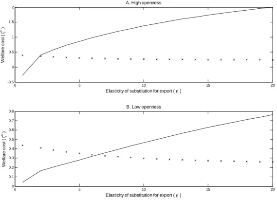
(Figure 1 about here)

In order to investigate further the robustness of the results for di¤erent values of , we

plot the welfare costs for the exchange rate rules and interest rate rules, for between 0.6

to 20 in Figure 1. For both types of monetary policy rules, we …x at 3 and GDP at

0 for all values of . As can be seen from the …gure, for the case of high openness, the

exchange rate rule is welfare superior to the interest rate rule for > 2. For the case of the

low openness, the exchange rate rule is welfare superior to the interest rate rule for > 7.

These values are within the range of the empirical estimates of the elasticity of substitution. Hence, the results in this paper suggest that high degree of openness by itself does not make an exchange rate rule to be welfare superior to an interest rate rule, when the expected utility of the representative household is used as the welfare criterion. In contrast, for high elasticity of substitution for export, an exchange rate rule can be welfare superior to an

(24)

interest rate rule, regardless of the degrees of openness. It is also worthwhile to note that the welfare costs of interest rate rules increase very rapidly as elasticity of substitution for export increases, especially for the case of high openness, while the welfare costs of exchange rate rules change by less as elasticity of substitution for export changes.

6 Conclusion

In this paper, we compare the welfare performances of exchange rate rules with interest rate rules. We develop a New Keynesian small open economy DSGE model for the analysis. We depart from the existing studies on exchange rate rules by using the expected lifetime utility of the representative household as the welfare criterion. We …nd that while an exchange rate rule delivers lower standard deviations of GDP and in‡ation compared to an interest rate rule when the degree of openness is high, an exchange rate rule is welfare inferior to an interest rate rule under benchmark parameterization. This is because an exchange rate rule delivers lower mean terms of trade, which leads to lower mean consumption and higher mean labor hours. However, for high elasticity of substitution for export, an exchange rate rule is welfare superior to an interest rate rule, regardless of the degree of openness, as the di¤erences in mean terms of trade for the two classes of rules become smaller.

The results in this paper suggest that elasticity of substitution for export, which can be thought of as the degree of competition in the export market, is more important than the degree of openness in deciding the welfare ranking between exchange rate rules and interest rate rules. They also suggest that an exchange rate rule can be a better monetary policy rule than an interest rate rule for a country that faces intense competition in the export market, which should be relevant for most emerging economies.

We conclude this paper by discussing the directions for future research. First, the paper can be extended to allow for incomplete pass-through of exchange rate. Studies such as

(25)

Devereux and Engel (2003) and Corsetti and Pesenti (2005) have shown that incomplete pass-through can alter the welfare ranking of monetary policy regimes. Second, the paper can be extended to incorporate "balance sheet e¤ects". Elekdag and Tchakarov (2007), for example, have shown that balance sheet e¤ects associated with liability dollarization can make it bene…cial for emerging markets to stabilize the exchange rate.

References

[1] Ascari, G., 2004. Staggered prices and trend in‡ation: some nuisances. Review of Eco-nomic Dynamics 7, 642-667.

[2] Bacchetta, P., van Wincoop, E., 2000. Does exchange rate stability increase trade and welfare? American Economic Review 90, 1093-1109.

[3] Ball, L. 1999. Policy rules for open economies. In Taylor J. (Eds.), Monetary Policy Rules. Chicago: University of Chicago Press, 127-144.

[4] Bergin, P., Shin, H., Tchakarov, I., 2007. Does exchange rate variability matter for wel-fare? A quantitative investigation of stabilization policies. European Economic Review 51, 1041-1058.

[5] Calvo, G.A., 1983. Staggered prices in a utility-maximizing framework. Journal of Mon-etary Economics 12, 383-398.

[6] Christiano, L.J., Eichenbaum, M., Evans, C., 2005. Nominal rigidities and the dynamic e¤ects of a shock to monetary policy. Journal of Political Economy 113(1), 1-45. [7] Clarida, R. Gali, J., Gertler, M., 1998. Monetary policy rules in practice: some

inter-national evidence. European Economic Review 42(6), 1033-1067.

[8] Clarida, R. Gali, J., Gertler, M., 2000. Monetary policy rules and macroeconomic sta-bility: evidence and some theory. Quarterly Journal of Economics 115. 147-180.

[9] Corsetti, G., Paolo, P., 2005. International dimensions of optimal monetary policy. Journal of Monetary Economics 52(2), 281-305.

[10] Devereux, M.B., Engel, C., 2003. Monetary policy in an open economy revisited: price setting and exchange rate ‡exibility. Review of Economic Studies 70, 765-783.

[11] Devereux, M.B., Engel, C., 2007. Expenditure switching versus real exchange rate stabi-lization: competing objectives for exchange rate policy. Journal of Monetary Economics 54, 2346-2374.

(26)

[12] Elekdag, S., Tchakarov, I., 2007. Balance sheets, exchange rate policy and welfare. Journal of Economic Dynamic and Control 31, 3986-4015.

[13] Hummels, D., 2001. Toward a geography of trade costs. Mimeo, Purdue University. [14] Julliard, C. 1996. Dynare : a program for the resolution and simulation of dynamic

models with forward variables through the use of a relaxation algorithm. CEPREMAP Working Paper 9602.

[15] Kim, J., Kim S., 2003. Spurious welfare reversals in international business cycle models. Journal of International Economics 60, 471-500.

[16] Kollmann, R., 2002. Monetary policy rules in the open economy : E¤ects on welfare and business cycles. Journal of Monetary Economics 49, 989-1015.

[17] Lai, H., Tre‡er, D., 2002. The gains from trade with monopolistic competition: speci…-cation, estimation, and mis-speci…cation. NBER Working Paper 9169.

[18] Lubik, T.A., Schorfheide, F. 2004. Testing for indeterminacy: An application to U.S. monetary policy. American Economic Review 94(1), 190-217.

[19] Lubik, T.A., Schorfheide, F. 2007. Do central banks respond to exchange rate move-ments? A structural investigation. Journal of Monetary Economics 54, 1069-1087. [20] Lucas, R., 1987. Models of business cycles. Yrjo Jahnsson Lectures Series. London:

Blackwell.

[21] McCallum, B.T., 1988. Robustness properties of a rule for monetary policy. Carnegie-Rochester Conference Series for Public Policy 29, 173-203.

[22] McCallum, B.T., 2005. A monetary policy rule for automatic prevention of a liquidity trap. NBER Working Paper 11056.

[23] McCallum, B.T., 2006. Singapore’s exchange rate-centered monetary policy regime and its relevance for China. Monetary Authority of Singapore Sta¤ Paper 43.

[24] McCallum, B.T., 2007. Monetary policy in East Asia; the case of Singapore. Bank of Japan Institute for Monetary and Economic Studies Discussion Paper 2007-E-10. [25] McCallum, B.T., Nelson, E.,1999. Nominal income targeting in an open-economy

opti-mizing model. Journal of Monetary Economics 43, 553-578.

[26] Monetary Authority of Singapore, 2001. Singapore’s Exchange Rate Policy.

[27] Parrado, E., 2004. Singapore’s unique monetary policy: how does it work? IMF working paper 04/10.

(27)

[28] Schmitt-Grohé, S., Uribe, M., 2003. Closing small open economy models. Journal of International Economics 61(1), 163–185.

[29] Schmitt-Grohé, S., Uribe, M., 2004a. Optimal simple and implementable monetary and …scal rules. NBER Working Paper No. 10253.

[30] Schmitt-Grohé, S., Uribe, M., 2004b. Solving dynamic general equilibrium models using a second-order approximation to the policy function. Journal of Economic Dynamics and Control 28, 755-775.

[31] Schmitt-Grohé, S., Uribe, M., 2005. Optimal …scal and monetary policy in a medium scale macroeconomic model: Expanded version. NBER Working Paper No. 11417. [32] Schmitt-Grohé, S., Uribe, M., 2006a. Comparing two variants of Calvo-type wage

stick-iness, NBER Working Paper No. 12740.

[33] Schmitt-Grohé, S., Uribe, M., 2006b. Optimal simple and implementable monetary and …scal rules: an expanded version. NBER Working Paper No. 12402.

[34] Schmitt-Grohé, S., Uribe, M., 2007. Optimal simple and implementable monetary and …scal rules. Journal of Monetary Economics 54, 1702–1725.

[35] Sutherland, A., 2005. Incomplete pass-through and the welfare e¤ects of exchange rate variability. Journal of International Economics 65, 375-399.

[36] Sutherland, A., 2006. The expenditure switching e¤ect, welfare and monetary policy in a small open economy. Journal of Economic Dynamic and Control 30, 1159-1182. [37] Taylor, J., 1993. Discretion versus policy rules in practice. Carnegie-Rochester

Confer-ence Series on Public Policy 39, 195-214.

[38] Woodford, M., 2003. Interest and prices: foundations of a theory of monetary policy. Princeton University Press, Princeton.

(28)

Table 1

Benchmark parameter values for high-openness economy

Parameter Description Value

Coe¢ cient of relative risk aversion 2

Subjective discount factor 0:99

Inverse of Frisch labor elasticity 1

Preference parameter for labor in utility 12:376

# Elasticity of substitution between value added and imported input 0:6

Elasticity of substitution for export 0:6

Share of domestic value added in production 0:58

Capital share in value added 0:3

v Elasticity of substitution across di¤erent variety of goods 6

Scale factor for export 0:391

Depreciation rate of capital 0:025

Capital adjustment cost 15

Price stickiness parameter 0:75

Steady state gross in‡ation rate 1

Extent of …nancial integration 0:0019

Persistence of technology process 0:9

Persistence of foreign in‡ation process 0:8

R _{Persistence of foreign interest rate process} _0:75

' _{Persistence of UIP shock} _0:5

Standard deviation of technology shock 0:01

Standard deviation of foreign in‡ation shock 0:005

R _{Standard deviation of foreign interest rate shock} _0:004

(29)

Table 2

Benchmark results

High openness Low openness

Exchange rate Interest rate Exchange rate Interest rate

rule rule rule rule

3.00 1.80 3.00 2.90 GDP 1.00 0.00 0.80 0.00 c _0.34 _-0.31 _0.37 _0.04 Mean Ct 0.97 2.01 0.19 0.57 Lt -0.54 -1.33 -0.10 -0.33 St 1.28 3.24 2.34 3.79 ut 0.09 0.18 0.15 0.02 Standard deviation GDPt 1.79 2.30 2.56 2.15 Ct 3.01 1.53 2.18 1.22 Lt 1.27 2.83 2.62 0.87 t 2.00 2.86 2.54 0.87 x t 7.25 25.90 12.72 28.65 m t 5.56 26.89 10.35 28.59 St 3.04 6.99 6.24 8.80 et 1.59 6.85 2.73 7.25

Notes: (1) The interest rates rules are given byln (Rt=R) = ln ( t= )+ GDPln(GDPt=GDP )

while the exchange rate rules are given byln ( et= e) = ln ( t= ) GDPln(GDPt=GDP ).

(2) In the optimized rules, and GDP are restricted to lie in the interval of [0,3]. (3) All

statis-tics are in percentage terms, except for the in‡ation rates, t, xt and mt , which are in annualized

(30)

Table 3

Results for the case of high elasticity of substitution for export

High openness Low openness

Exchange rate Interest rate Exchange rate Interest rate

rule rule rule rule

3.00 3.00 3.00 3.00 GDP 0.00 0.50 0.20 0.30 c 0.27 0.68 0.29 0.38 Mean Ct 0.37 -0.01 0.02 -0.07 Lt -0.18 -0.04 0.10 0.14 St 0.11 0.25 0.26 0.68 ut 0.03 0.20 0.07 0.12 Standard deviation GDPt 2.76 4.32 2.52 3.32 Ct 3.57 3.03 2.87 2.11 Lt 2.21 5.56 1.67 3.74 t 1.11 2.96 1.82 2.30 x t 4.45 8.02 7.75 15.39 m t 2.20 8.21 5.31 15.67 St 0.98 1.78 2.17 3.63 et 0.84 2.29 1.50 4.06

Notes: (1) The interest rates rules are given byln (Rt=R) = ln ( t= )+ GDPln(GDPt=GDP )

while the exchange rate rules are given byln ( et= e) = ln ( t= ) GDPln(GDPt=GDP ).

(2) In the optimized rules, and GDP are restricted to lie in the interval of [0,3]. (3) All

statis-tics are in percentage terms, except for the in‡ation rates, t, xt and mt , which are in annualized

(31)

0 5 10 15 20 -0.5 0 0.5 1 1.5 2

Elasticity of substitution for export (η )

W e lfa re c o s t ( ζ c ) A. High openness 0 5 10 15 20 0 0.1 0.2 0.3 0.4 0.5 0.6 0.7 0.8

Elasticity of substitution for export (η )

W e lfa re c o s t (ζ c ) B. Low openness

Figure 1: Welfare costs as elasticity of substitution for export varies Legend: Straight lines: Interest rate rules; Crosses: Exchange rate rules

(32)

出席國際學術會議心得報告

計畫編號

NSC

95-2415-H-002-020

計畫名稱臺灣和新加坡的貨幣政策﹕它們不一樣嗎﹖為什麼﹖ 出國人員姓名服務機關及職稱張永隆國立台灣大學經濟學系暨研究所助理教授會議時間地點 Held at Montreal, Canada on June 14-16, 2007

會議名稱 13th

International Conference on Computing in Economics and Finance 發表論文題目 Revisiting Exchange Rate Rule

一、參加會議經過我在 2007 年 6 月 14 日在此國際會議的一個 session 發表此計劃的論文。另外﹐我也在其它 sessions 聽到和這個計劃相關領域的最新研究﹐並在與會間和多位外國學者交流。二、與會心得我在發表論文時得到在座聽眾的許多寶貴意見﹐並在其它 sessions 得到領域裡最新發展的訊息。和外國學者交流也收穫甚多。

(33)

Can Exchange Rate Rules be Better than Interest

Rate Rules?

Wing Leong Teo

y

Department of Economics

National Taiwan University

March 11, 2008

Abstract:

We develop a New Keynesian small open economy model to compare the welfare perfor-mances of two classes of monetary policy rules: exchange rate rules and interest rate rules. The expected lifetime utility of the representative household is used as the welfare criterion. The model is solved using second-order approximation methods. We …nd that under bench-mark parameterization, an exchange rate rule delivers lower standard deviations of GDP and in‡ation compared to an interest rate rule, when the economy has a high degree of openness. However, despite that, an exchange rate rule is welfare inferior to an interest rate rule since it delivers lower mean terms of trade, which leads to lower mean consumption and higher mean labor hours. On the other hand, when the elasticity of substitution for export is high, an exchange rate rule is welfare superior to an interest rate rule, regardless of the degree of openness, as the di¤erences in mean terms of trade for the two classes of rules become smaller.

Keywords: Exchange rate rules, interest rate rules, monetary policy, welfare comparison, small open economy

JEL Classi…cation: E52, F41

This paper has been previously circulated under the title: Revisiting Exchange Rate Rule. I would like to thank participants at the 2007 Society of Computational Economics Annual conference for useful discussions. Financial support from the National Science Council of Taiwan, grant NSC 95-2415-H-002-020 is gratefully acknowledged.

y_{Department of Economics, National Taiwan University, 21 Hsu Chow Road, Taipei 100, Taiwan. Phone:}

(34)