蜂巢式OFDMA系統之效能改進技術

國 立 交 通 大 學

電信工程學系

博 士 論 文

蜂巢式 OFDMA 系統之效能改進技術

Performance Improvement Techniques for

Cellular OFDMA Systems

研究生：傅宜康

指導教授：沈文和 教授

蜂巢式 OFDMA 系統之效能改進技術

Performances Improvement Techniques for

Cellular OFDMA Systems

研究生：傅宜康

Student: I-Kang Fu

指導教授：沈文和 博士 Advisor:

Dr.

Wern-Ho

Sheen

國立交通大學

電信工程學系

博士論文

A Dissertation

Submitted to Institute of Communication Engineering

College of Electrical and Computer Engineering

National Chiao Tung University

in Partial Fulfillment of the Requirements

for the Degree of Doctor of Philosophy

in

Communication Engineering

Hsinchu, Taiwan

To my family – S. L. Fu, S. C. Chang, I. L. Fu, L. Y. Lee, Z. L. Kuo

Special thanks to my advisor – Prof. W. H. Sheen and my friends in IEEE 802.16 Working Group.

Abstract

OFDMA (Orthogonal Frequency Division Multiple Access) is one of the key multiple access techniques to enable broadband wireless transmission for next generation mobile cellular systems. In order to improve and investigate the performance of cellular OFDMA systems, this dissertation proposes several advanced techniques and part of the designs have been adopt by the international standard organization. The downlink capacity of cellular OFDMA systems is first investigated through the proposed mathematical analysis. The proposed analysis is general and incorporates the effects of propagation environment, cell size, frequency reuse factors, reuse partitioning (fractional frequency reuse), antenna setups and etc. The numerical results show that the downlink capacity of cellular OFDMA system can be significantly improved by reuse partitioning and intra-cell frequency reuse. Then, an improved FBSS (Fast Base Station Switching) handover technique is proposed to improve the packet loss rate for the handover users. Simulation results show that the proposed technique can significantly reduce the packet loss rate for the users during FBSS at a slight expense on system capacity. In addition, a recent advance in multi-hop relay technology is introduced and investigated, and the benefit on user throughput enhancement and coverage extension by relay deployment are justified by simulation results. But it also shows that the capacity may not be improved by deploying relay stations with respect to the cellular OFDMA system with no relay. In order to improve the capacity of multi-hop cellular OFDMA systems, advanced frequency planning (reuse) techniques and path selection techniques are investigated and proposed. Compare to existing techniques, the proposed frequency planning (reuse) technique can lead to 60.87% ~ 137.75% capacity improvements under the guaranteed coverage. In addition, simulation results also show that further 16.87% ~ 26.31% capacity improvement can be achieved by advanced path selection based on proposed SINR prediction technique.

摘 要

OFDMA (Orthogonal Frequency Divisional Multiple Access)被視為是下一代行動通 訊系統之核心技術，其重要性在可於高速資料傳輸時有效解決符際干擾(Inter Symbol Interference, ISI)的問題。以 OFDMA 為核心之蜂巢式無線接取網路將會 是下一代無線寬頻通訊系統之核心。為了提升及探討蜂巢式 OFDMA 系統之效 能，本論文提出了多種技術以探討或提升系統之效能。首先，本文提出了一套新 型之數學分析方法以探討蜂巢式 OFDMA 系統之下鏈系統容量，且該分析方法可 廣泛納入細胞涵蓋範圍、頻率重用係數、頻率分段重用(reuse partitioning)、天線 組態等效應，藉由分析數值結果顯示透過頻率分段重用技術搭配細胞內之頻率重 複使用可顯著的提升系統容量。本論文並進一步提出一套改良型之快速基地台切 換(Fast Base Station Switching, FBSS)技術，其設計在於結合頻率分段重用技術以 預留部分干擾較輕微之通道以提升換手中的使用者之訊號品質。模擬結果顯示所 提出之技術可可大幅減低(93.6%)使用者在換手過程中所遭受之封包遺失率，且 僅些微的損耗(5.82%)部份系統容量。此外，本論文介紹並探討了一種可應用於 蜂巢式 OFDMA 系統之 Multi-hop Relay 技術標準：IEEE 802.16j，並透過電腦模 擬探討採用 Multi-hop Relay 技術對於系統整體效能之影響。模擬結果顯示於系統 加入中繼站(Relay Station)可有效提升使用者傳輸速率及系統涵蓋範圍，但結果 亦顯示系統容量有可能因為資料轉傳所額外消耗的資源而惡化。為了有效提升 Multi-hop 蜂巢式 OFDMA 系統之容量，本論文進一步提出了新型之頻率規劃及 重複使用技術以及以 SINR 預測為基礎之新型路徑選擇技術。相較於現有之頻率 規劃方法，本文所提出之方法可大幅(60.87%~137.75%)提升系統容量且不影響系 統有效之涵蓋範圍，而模擬結果亦顯示所提出之路徑選擇方法可進一步提升 16.87%~26.31%之系統容量。

Table of Contents

List of Figures………..………ii

List of Tables………..iii

1. Introduction………1

2. Capacity Improvement Techniques for Cellular OFDMA Systems….6

2.1. Downlink Capacity Analysis of Cellular OFDMA Systems………6

2.2. Capacity Improvement Techniques for Cellular OFDMA Systems………20

3. An Improved Fast Base Station Switching Technique for Cellular

OFDMA Systems………25

3.1. Fast Base Station Switching in IEEE 802.16 network………..25

3.2. An Improved Fast Base Station Switching Technique for Cellular OFDMA Systems………..31

4. Multi-hop Cellular OFDMA Systems………40

4.1. IEEE 802.16j Multi-hop Relay Network………41

4.2. Coverage Planning for Multi-hop Cellular Networks………46

4.3. Performances Improvement by Multi-hop Relay………...53

5. New Frequency Reuse Techniques for Multi-hop Cellular OFDMA

Systems………...61

5.1. A New Frequency Planning Technique for Multi-hop Cellular OFDMA Systems………61

5.2. A Novel Measurement and Reporting Mechanism for IEEE 802.16j Multi-hop Relay Network………72

6. A New Path Selection for Multi-hop Cellular OFDMA System based

on SINR Prediction……….78

6.1. A Novel SINR Prediction Mechanism for Multi-hop Relay Systems……78

6.2. A New Path Selection Criterion based on SINR Prediction………82

7. Conclusions………93

List of Figures

Figure 1 - Cellular Structure……….2 Figure 2 - (a) Geometry of interfering cells (Q=18) (b) Geometry of the reference cell

and the interfering cell q ………....8

Figure 3 - Example sub-carrier allocation and permutation in OFDMA systems……10 Figure 4 - The concept of reuse partitioning:(a) divide the cell into Z concentric regions and (b) serve each region by corresponding frame zone with different K_z………….11 Figure 5 - Downlink capacity of multi-cell OFDMA system with single MCS-class ...22 Figure 6 - Downlink capacity of multi-cell OFDMA system with multiple MCS-classes ………23 Figure 7 - Downlink capacity of multi-cell OFDMA system with reuse partitioning…24 Figure 8 - Cell structure, received radio-link signals, diversity set membership and Anchor BS selection of an MS involved in FBSS in IEEE 802.16e………..27 Figure 9 - The message flow of FBSS in IEEE 802.16e……….28 Figure 10 - A simplified IEEE 802.16e TDD frame structure with (a) regular K = 4 resource zone, and (b) regular K = resource zone and 4 K =7 RP zone………….32 Figure 11 - Reuse partitioning cell structure, received radio-link signals, diversity membership, Anchor BS selection and scheduled zones of an MS in FBSS with reuse partitioning……….34 Figure 12 - The performances of FBSS with reuse partitioning………..…38 Figure 13 - (a) Packet loss rate reduction and (b) cell throughput penalty………39 Figure 14 - (a) The system architecture and (b) the frame structure for IEEE 802.16j multi-hop relay network……….44 Figure 15 - A multi-hop cellular network with RS deployed within the coverage of BS ………53 Figure 16 - The proposed RS deployment method: (1) to have LOS with signal source and (2) to have NLOS with interference source………....54 Figure 17 - (a) CDF of downlink received signal quality and (b) the downlink cell capacity………58 Figure 18 - (a) The CDF of uplink MS transmit power and (b) uplink cell capacity ………60

Figure 19 - A reference multi-hop cellular structure……….62

Figure 20 - The frequency planning technique proposed in literatures [44,45]………63

Figure 21 - The frequency planning technique proposed in literatures [46-49]………64

Figure 22 - Proposed frequency planning technique based on “sub-cell”……….66

Figure 23 - System capacity by given different access zone ratio (η)………69

Figure 24 - System capacity under different frequency planning techniques…………70

Figure 25 - CDF of the received signal quality (SINR)………70

Figure 26 - MCS percentage in access links………..71

Figure 27 - Examples on (a) proposed measurement mechanism, and the corresponding transmission opportunities for the RSs with the (b) same reference signal and (c) different reference signals………..73

Figure 28 - Instructing R-amble transmission by RS-CD message, (b) the corresponding operation of the RSs and (3) the flexibility for instruction………74

Figure 29 - Proposed method to synchronize the R-amble transmission/measurement opportunities in different MR-cells………76

Figure 30 - An example to illustrate the proposed SINR prediction method…………80

Figure 31 - Path selection problem in multi-hop relay systems………83

Figure 32 - Interfering scenario when 2nd path is selected………85

Figure 33 - Interfering scenario when 3rd path is selected……….86

Figure 34 - Capacity for each path selection criteria in Scenario #1……….91

Figure 35 - Capacity for each path selection criteria in Scenario #2……….92

List of Tables

Table 1 - OFDMA parameters used in numerical results………21

Table 2 - Parameters for system-level simulation……….36

Table 3 - A typical format of link budget for downlink OFDMA system………46

Table 4 - A link budget example for MR-BS in downlink OFDMA system…………51

Table 5 - A link budget example for RS in downlink OFDMA system………52

Table 6 - SINR prediction results for different radio resource reuse patterns………81

Chapter 1

Introduction

Advances in mobile communication technologies in last decade have dramatically changed human’s lives. From mobile telephony to mobile Internet, people are able to access information anytime and anywhere. Today, people can make reservation for their dinner by mobile phone when they are driving on high way, or they can receive/reply some urgent emails by wireless Internet when they are traveling on the train in a foreign country. Such a convenience further triggers more people’s expectation on more fruitful applications by wireless communication. Therefore, higher transmission rate, ubiquitous network connectivity, lower access fee, seamless service and etc. are the common desires on next generation mobile communication systems by the people around the world [1].

One of the most popular technologies used by mobile communication systems is the radio transmission technology, i.e. transmitting the information signal through radio waves. Thanks the advances in semi-conductor technologies, the cost on manufacturing the devices for radio transmission and signal processing is much lower than before and it makes the mobile communication products be very popular around the world in a very short time. However, the radio frequency spectrum is a very scarce resource and always controlled by the government in each country. The privilege to provide mobile communication services via a specific frequency bandwidth (i.e. licensed-band) is very expensive, for example, some companies spend more than ten billion Taiwan dollars to acquire the privilege to perform the services via 3G/3.5G systems. Therefore, there will be many technical challenges to serve more users with

higher transmission rate by such a scarce radio bandwidth.

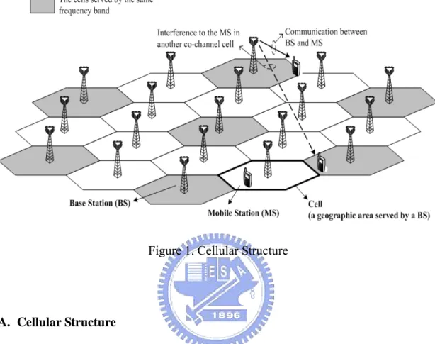
Figure 1. Cellular Structure

A. Cellular Structure

The most general resolution to the aforementioned problem is reusing the same frequency bandwidth in different geographic area, which is called frequency reuse [2]. In order to manage the interference when the same bandwidth is reused to transmit different signals, the cellular structure as shown in Figure 1 is used as a tool to determine the area served by each frequency band. Note that a cell is defined as the coverage served by a base station (BS). By separating the cells which use the same frequency (called co-channel cells) far enough, the interference will degrade to a very low level when received by the mobile station (MS) or BS in the co-channel cells, so that the received signal quality in each cell can be higher than an acceptable level for normal communication. In the modern mobile communication systems which operate

deploying its radio access network.

B. OFDMA (Orthogonal Frequency Division Multiple Access)

In addition, next-generation mobile communication is envisaged to support multimedia services over a wide variety of operation environments: indoors, outdoors, low-mobility, high-mobility, etc. Data rate up to several tens Mbps is essential in order to support a multitude of services with guaranteed QoS. Meanwhile, very high spectrum efficiency, at least one order in magnitude higher than the 3G systems, is needed to best utilize the very scarce radio spectrum in the future. One key challenge in designing such a system is to overcome inter-symbol interference (ISI) incurred by high-data-rate transmission. Furthermore, technology advancements in multiple access techniques, intelligent antenna systems, coding/decoding, etc. have to be exploited fully so as to achieve the targeted spectrum efficiency [3].

OFDM (orthogonal frequency division multiplexing) is an effective modulation/multiplexing scheme to combat ISI in a high-data-rate environment, where frequency band is divided into sub-carriers and over which data are transmitted in parallel. Through the use of cyclic-prefix, ISI can be avoided completely in a multi-path channel as long as the cyclic-prefix is larger than the maximum delay spread [4].

OFDM can also be used as an effective multiple access scheme [5]. In particular, OFDMA (orthogonal frequency division multiple access), a form of combining OFDM and FDMA (frequency division multiple access), has been widely regarded as one of the most promising multiple access schemes for the next generation systems [2,6]. OFDMA has been adopted in the 3GPP-LTE (long term evolution) down-link [7

In this dissertation, the system combines with cellular structure and OFDMA (i.e. cellular OFDMA system) will be first investigated in Chapter 2 and Chapter 3. In Chapter 2, the design tradeoffs on the cellular structure for cellular OFDMA systems will be investigated by a proposed mathematical analysis. In Chapter 3, a popular handover mechanism called fast base station switching (FBSS) is introduced and an improved version is also proposed.

C. Multi-hop Relay

When the system operators try to upgrade their cellular OFDMA networks to support a much higher transmission rate, there will be a transmit power problem. For example, ten times in transmission rate will result in more than ten times in transmit power in order to meet the required signal to interference plus noise ratio (SINR) [9]. Since the transmit power cannot be increased unlimitedly due to the hardware cost or battery life of a MS, the coverage holes may exist between adjacent BSs.

Traditional solution to this problem is to deploy additional BSs or repeaters to serve the coverage holes. Unfortunately, the cost of BS is very high and the wire-line backhaul may not be available everywhere. Repeater, on the other hand, has the problem of amplifying interference and has no intelligence of signal control and processing. Recently, relay station (RS) that receives and forwards signals from source to destination through radio has been developed as a more cost-effective solution. Since RSs do not need a wire-line backhaul, the deployment cost of RSs will be much lower than that of BSs. Meanwhile, RS can decode the signal from the source and forward it to the destination. Intelligent resource scheduling and cooperative transmission can be applied to obtain better system performance [10]. In Chapter 4, an overview of modern advances on multi-hop relay network and the

relay with respect to the cellular OFDMA systems with no relay is studied in this chapter with simulation. In Chapter 5, a new frequency planning technique with a novel measurement and report mechanism for multi-hop cellular OFDMA systems (i.e. the cellular OFDMA systems with multi-hop relay technology) are proposed. A novel path selection based on SINR prediction is proposed in Chapter 6 and, finally, the conclusion is provided in Chapter 7.

Chapter 2

Capacity Improvement Techniques for Cellular

OFDMA Systems

OFDMA (orthogonal frequency division multiple access) is widely regarded as a key multiple access technology for broadband mobile radio systems, and has been adopted in the 3GPP-LTE (long term evolution) down-link and IEEE 802.16e specifications. This chapter analyzes the down-link capacity of multi-cell OFDMA systems under a randomized multiple access interference, a result of applying random sub-carrier allocation among cells/sectors. A mathematical analysis is proposed in Section 2.1 to efficiently evaluate the system capacity which is obtained through mainly time-consuming computer simulations previously. The analysis is general enough to take into account the effects of propagation environment, cell size, frequency reuse factor, reuse partitioning (fractional frequency reuse), antenna set-ups, etc. In Section 2.2, an OFDMA system resembling that specified in IEEE 802.16e is analyzed to illustrate how the analysis can be used to optimize the design of a system to achieve the highest capacity.

2.1 Downlink Capacity Analysis of Cellular OFDMA

Systems

The capacity of OFDMA systems has recently been investigated in the literatures. In [11] and [12], the up- and down-link capacity of multi-cell OFDMA systems was investigated through computer simulations. The system capacity was compared for

downlink were simulated, and their results indicated that the system suffers a severe degradation from using a large cell radius and/or having high loading in the interfering cells. In [14], the downlink capacity of multi-cell OFDMA was compared with CDMA (code division multiple access) through simulations. Numerical results show that OFDMA can achieve higher capacity when operating in the Rayleigh fading channel.

Instead of resorting time-consuming computer simulations, this chapter aims to provide an efficient mathematical analysis on the downlink capacity of multi-cell OFDMA systems with randomized multiple access interference (MAI), a result of applying random sub-carrier allocation among cells/sectors which has been adopted in IEEE 802.16e [8]. Efficient capacity evaluation is indispensable for optimal system design that gives the best tradeoff among different system parameters. The analysis is general enough to include the effects of reuse partitioning (fractional frequency reuse), different antenna set-ups and multiple modulation and code schemes (MCS).

2.1.1 Cellular OFDMA System Model

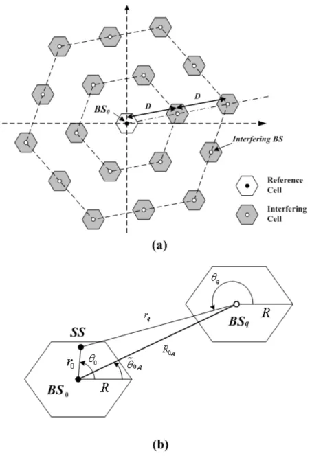
Figure 2(a) depicts the considered multi-cell architecture. The reference base station (BS) is denoted asBS , and the interfering BSs are denoted as ₀ BS , q = 1, _q

2 … Q, where Q is the number of the interfering BSs. Cell radius R is the same for every BS, and the distance between adjacent interfering BSs is given byD= 3K R⋅ ,

where K is the reuse factor (cluster size) [15]. K is a key system parameter that balances link performance and system capacity. Different K values are investigated in Section IV.

OFDMA is a combination of OFDM and FDMA, where frequency band is divided into orthogonal sub-carriers, and these sub-carries are grouped (allocated) together to

consist of a channel to serve users. In real systems, sub-carriers in channels are not overlapping in a cell/sector so as to avoid intra-cell/sector interference [7,8]. As a

Figure 2. (a) Geometry of interfering cells (Q=18) (b) Geometry of the reference cell and the interfering cell q

consequence, the co-channel inter-cell/sector interference becomes the main limiting factor to the system capacity in a multi-cell deployment, given a channel bandwidth.

A. Diversity Sub-carrier Allocation and Permutation

Two types of sub-carriers allocation to a channel are popular in real OFDMA systems [7,8]. One is diversity allocation, where sub-carriers in a channel are distributed over the entire frequency band, and the other is adjacent allocation, where sub-carriers are adjacent to each other. Diversity allocation is designed to obtain frequency diversity at link level, and adjacent allocation is meant to exploit multi-user diversity through frequency-selective scheduling for low-mobility users at system level [16]. In this work, we are only concerned with diversity allocation.

In diversity allocation, the way of allocating sub-carriers into a channel is often

permuted randomly among cells/sectors so as to randomize the inter-cell/sector MAI.

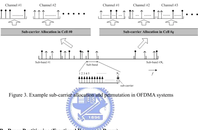
It eliminates the most severe interfering scenario in a multi-cell environment like in a narrow-band system and makes the worst-case network planning not necessary. For example, in the IEEE 802.16e OFDMA downlink, sub-carrier allocation is done with a pseudo-randomly sub-carrier mapping process, called sub-carrier permutation [8]. The basic idea is explained with Figure 3 as follows. Firstly, the available sub-carriers are divided into N sub-bands, with each of them consisting of _S N adjacent _C

sub-carriers. Then each of the sub-carriers in a sub-band is allocated to one of N C

channels (called sub-channel in IEEE 802.16e) in a non-overlapping way. Thus, each of the channels consists exactly of N sub-carriers. For users in the same cell/sector, S

they use different channels so that there is no intra-cell/sector interference. Secondly, the way of allocating sub-carriers into sub-channels is permuted pseudo-randomly in different cells/sectors in order to randomize the inter-cell/sector interference. The sub-carrier allocations for different cells are illustrated in Figure 3. In the IEEE 802.16 OFDMA system, the sub-carrier permutation of a cell/sector is fixed and determined by the cell/sector ID [8]. To facilitate analysis, nevertheless, sub-carrier

following. With this arrangement, we say that the inter-cell/sector MAI has been randomized completely, and, therefore, each sub-carrier/channel experiences the same statistical characteristics of MAI [17,18].

Figure 3. Example sub-carrier allocation and permutation in OFDMA systems

B. Reuse Partitioning (Fractional Frequency Reuse)

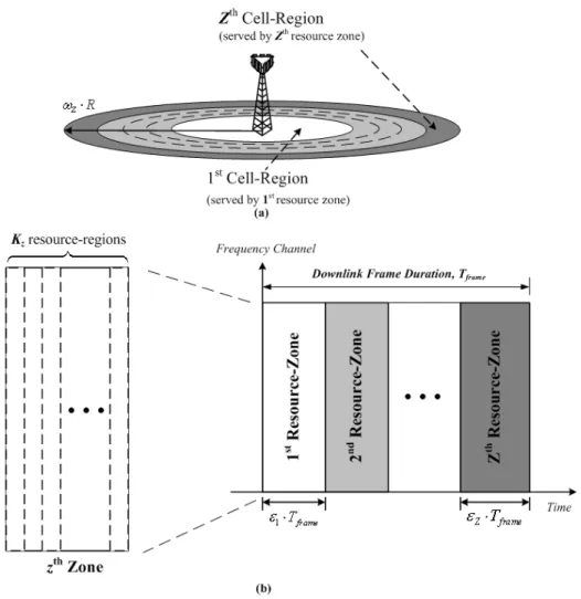
Reuse partitioning is a cell structure, where a regular cell is divided (ideally) into two or more concentric cell-regions, each with a different frequency reuse factor ( K ) [19]. By allowing the inner cell-regions to use a smaller reuse factor leads to a higher system capacity, as compared to the regular cell structure where the same reuse factor is used for the entire cell.

Figure 4 illustrates the concept of reuse partitioning with a TDD frame structure. In Figure 4(a), a regular cell is divided into Z cell-regions with the z-th region denoted by

{

ωz−1R< ≤r0 ωzR, 0<θ0≤2π

}

, where ωz−1≤ωz, ω0 = , 10 ωZ = , and 1 z Z≤ ≤ .

shown in Figure 4(b), whereK is the reuse factor for z-th cell-region. Finally, each z

of the resource-region is allotted to BSs according to the designated reuse factor and cell regions.

Figure 4 The concept of reuse partitioning: (a) divide the cell into Z concentric regions and (b) serve each region by corresponding frame zone with different Kz

C. Antenna Setups

Different antenna configurations have been used to increase system capacity and/or link quality of a cellular system. Two antenna configurations are to be considered, including 3-sector antenna and switched-beam smart antenna. For the 3-sector

antenna, the antenna pattern of each sector is the one specified in [20]

( )

(

)

2 , 18 14 min 12 , 20 , 1, 2,3 7 j j dB G θ θ ϕ dBi j π ⎡ ⎛ _{⋅ −} ⎞ ⎤ ⎢ ⎜ ⎟ ⎥ = − = ⎢ ⎜ ⎟ ⎥ ⎝ ⎠ ⎣ ⎦ , (2.1)

where − < −π θ ϕ_j ≤ , π ϕ_j is the steering direction of the antenna for j-th sector,

which are 0_{, 2 3}π _{and 4 3}π , respectively.

For the switched-beam smart antenna, the linear equally spaced (LES) array with omni-directional antenna elements is employed to form a number of fixed beams to cover different area of a cell, and users are served by the beam with the highest gain [21]. The j-th beam pattern is given by [22]

( )

(

)

(

)

2

sin cos cos

2

sin cos cos

2 j j j Wd G d β _{ϕ θ} θ β _{ϕ θ} ⎛ ₋ ⎞ ⎜ ⎟ ⎝ ⎠ = ⎛ ₋ ⎞ ⎜ ⎟ ⎝ ⎠ , (2.2)

where ϕ_j is the steering direction of j-th beam, d is the distance between antenna

elements, W is the number of antenna elements, β =2π λ is the phase

propagation factor, and λ is the wavelength. In the following, the “sector” and “beam” will be used interchangeably.

Two extreme cases of channel reuse among sectors (beams) of a cell are to be considered. One is that different sectors use different set of channels, i.e., channels are not reused among sectors (no-reuse), and the other is that all the channels are reused in all sectors (full-reuse). Because of the non-perfect antenna pattern, there will be intra-cell interference when channels in the full-reuse case.

For easy presentation, the considered cell architecture will be described by the vector

(

{

K K₁, ₂⋅⋅⋅K_Z

}

, ,1/J J

)

or

(

{

K K₁, ₂⋅⋅⋅K_Z

}

, ,1J

)

, where Kz is again the

sector. In other words, “1/ J ” denotes the no-reuse case, and “1” denotes the full-reuse case.

2.1.2 Capacity Analysis of Cellular OFDMA Systems

The downlink capacity of the power-controlled multi-cell OFDMA system is analyzed in this section. In the power-controlled system, the BS’s transmit power toward a particular user is controlled to just meet the link performance requirement of a modulation and code scheme (MCS), and hence reducing the interference to the co-channel users. More than one MCS-class is considered in the analysis.

Three common assumptions are made to facilitate the analysis. First, users are distributed uniformly over each cell-region of the cell/sector. Second, user is served by the sector (beam) with highest received power. And, third, user is ideally power controlled to just meet the required SINR.

Consider a user located at ( , )r₀ θ₀ in Figure 2(b), served by the z-th cell-region in

the j-th sector (beam) of BS and using the u-th MCS-class in a specific channel. For ₀

convenience, each user is assumed to use one channel only. Since all channels look the same to a user in the diversity sub-carrier allocation, there is no need to differentiate which channel is used by a user.

In the power-controlled systems, the received SINR of the user is controlled to meet to the target value ρ_u,

( )

0 , , 0 0 0, 0 0 0 0 ( , ) ( ) ( , ) j u z j u z p r G L r I r N θ θ ρ θ ⋅ ⋅ = + , (2.3)

where p_{j u z, ,} ( , )r₀ θ₀ is the downlink transmit power for the user, G_0,j

( )

θ₀ is the

antenna gain toward the direction θ₀, L r is the propagation loss, and ₀( )₀ I r_z( , )₀ θ

might be different for different j in the case of switched-beam smart antenna, and that is the reason why we need to differentiate the beam where the user is located in. The propagation loss L r is modeled as ₀( )₀

0( )0 0 0

l

L r = ⋅A r− ⋅ , (2.4) χ

where A is a constant determined by the path-loss model, l is the path-loss

exponent, and χ₀ is a log-normal random variable with zero mean and variance 2

dB

σ

in dB. The effect of small-scale multi-path fading is included in determining the link performance ρ_u, and thus is not explicitly treated here. From Equation (2.3), the required transmit power for the user is given by

(

)

( )

0 0 , , 0 0 0 0 0, 0 ( , ) ( , ) u z j z u l j I r N p r A r G ρ θ θ χ θ − ⋅ + = ⋅ ⋅ ⋅ . (2.5)

The analysis consists of three steps. Firstly, we obtain the average transmit power

, , , , ( , )0 0

j z u j z u

p = ⎣E p⎡ r θ ⎤_{⎦ for a particular MCS-class user who is located uniformly}

over the z-th cell-region of the j-th sector (beam), where E

[ ]

⋅ denotes the operation

of taking average. Secondly, the total transmission rates of the u-th MCS-class users in z-th cell-region of the j-th sector is calculated by

, , z u u S j z u z OFDM m c N M K T ε ⋅ ⋅ bps, (2.6)

where Mj z u_{, ,} is the total number of user in z-th cell-region of the j-th sector using the

u-th MCS-class, m and _u c are the bit number carried by the signal constellation _u

and the coding rate, respectively, ε is the ratio of the percentage of frame duration z

for serving the users in z-th cell-region as depicted in Figure 4(b), and TOFDMis the

, , 1 1 1 bps/cell J Z U u u S z j z u j z u z OFDM m c N C M K T ε = = = =

∑∑∑

⋅ ⋅ (2.7)

where U is the number of MCS-classes, and

, ,1 , , , ,1 , , _{, ,} , , ₁ , , _{, , ,} 1 , , _, 1 , , arg max subject to , 1 . j z j z U U z u u S j z j z U _{j z u} M M u z OFDM U j z u _{j z u T j} u U j z u _{C j} u m c N M M M K T M E p P j J M N ε ⎡ ⎤ ⎣ ⎦ = = = ⎧ ⎫ ⎡ _{⎤ = ⎨ ⋅ ⎬} ⎣ ⎦ _{⎩ ⎭} ⎧ _{⋅ ⎡ ⎤≤} ⎪ ⎣ ⎦ ⎪ _{≤ ≤} ⎨ ⎪ _≤ ⎪⎩

∑

∑

∑

, (2.8)

where P and _{T j,} N_{C j,} are the transmit power and number of channels allotted to the j-th sector, respectively. The first constraint in Equation (2.8) is due to the maximum

transmit power P , and the second is due to the maximum number of channelsT j_, NC j, .

2.1.2.1 Evaluation of E p⎡⎣ j z u_{, ,} ⎤⎦

Again, consider a user located at ( , )r₀ θ₀ in z-th region of the j-th sector ofBS , ₀

using the u-th MCS-class. E p⎡⎣ j z u_{, ,} ⎤⎦ , by definition, is given by

(

)

( )

( )

( )

( )

(

)

(

) ( )

0 0 0 0 , , _, 0 0 0, 0 ( ) , , 0, 0, 0 0 0 1 1 1, 1 0, 0 0 0 0 0 0 0 0 0 , , z z z z z z z j z u _r u l j Q J J q l l T v q v q q q v v q v v v j u l C j j j I r N E p E E A r G P G A r P G A r N E N G A r r f r dr d θ θ ρ χ θ θ χ θ χ ρ θ χ θ λ θ θ − − − = = = ≠ − − ⋅ ⎡ ⎡ + ⎤⎤ ⎡ ⎤ = ⎢ ⎢ ⋅ ⎥⎥ ⎣ ⎦ _{⎢ ⋅ ⋅ ⋅ ⎥} ⎢ ⎥ ⎣ ⎦ ⎣ ⎦ ⎡⎛ ⎞ ⋅ ⋅ ⋅ ⋅ + ⋅ ⋅ ⋅ ⋅ + ⎢⎜ ⎟ ⎢⎝ ⎠ = ⎢ ⋅ ⋅ ⋅ ⋅ ⋅ ⋅ ⋅ ⋅ ⋅ ⎢⎣

∑∑

∑

χ χ 1 2 0 z z R R ω π ω− ⋅ ⋅ ⎡ ⎤⎤ ⎢ ⎥⎥ ⎢ ⎥⎥ ⎢ ⎥⎥ ⎢ _⎥⎦⎥ ⎣ ⎦

∫ ∫

,(2.9)

where χ is the vector of Q+1 independent random variables

0 1 2 Q

χ χ χ χ

⎡ ⎤

⎣ … ⎦that characterize the shadowing effect from the interfering cells,

( ) ,z

q T v

P is the total transmit power of

z

q

BS over its v-th sector, _,

( )

z z q v q

G θ is the

indicator function to indicate that if the location is served by j-th sector, that is,

( )

{

( )

}

( )

{

}

0, 0 0 0, 0 1 arg max 0 arg max v v j v v if j G if j G θ λ θ θ ⎧ ₌ ⎪ = ⎨ ⎪ ≠ ⎩ . (2.10)

(

0 0

)

(

)

1 2 , j j

f r θ = a ⋅πR − is the density function of user location in a sector, where

( )

2 0 0 0 1 2 j j a = _π⋅

∫

πλ θ dθ . z q r , z q θ , z q r and _0, z q

R are the geometrical parameters

when reuse factor Kz is selected as indicated in Figure 2(b). In Equation (2.9), the

term

( )

(0) , 0, 0 0 0 1, 1 J l T v v v v j C P G A r N θ χ − = ≠ ⋅ ⋅ ⋅ ⋅

∑

(2.11) is the intra-cell interference in the intra-cell frequency reuse case which is equal to zero when no channel is reused in the same cell.

The first step of the derivation is to evaluate

0,0 j z u, ,

rEθ ⎡⎣p ⎤⎦ , which can be rewritten as

( )

( )

( )

( )

( )

( )

1 0 0 ( ) , , 2 _{1 1 0} , , ₀ 2 0 0 0 , 0, 0 0 0 (0) , 0, 0 0 0 2 _{1, 0} 0 0, 0 0 0 z z z z z z _z z Q J q l T v q v q q q R _{q v j} u j z u _R l r C j j J l T v v v v j j u l C j j P G A r E p r dr d N G A r a R P G A r N G A r a ω π ω θ π θ χ λ θ ρ _θ π θ χ θ χ _{λ θ} ρ π θ χ − − ⋅ _{= =} − ⋅ − = ≠ − ⋅ ⋅ ⋅ ⋅ ⎡ ⎤ = ⋅ ⋅ ⋅ ⎣ ⎦ _{⋅ ⋅ ⋅ ⋅ ⋅} ⋅ ⋅ ⋅ ⋅ + ⋅ ⋅ ⋅ ⋅ ⋅ ⋅ ⋅

∑∑

∫ ∫

∑

∫

( )

( )

1 1 0 0 0 2 2 ₀ 0 0 0 2 0 0, 0 0 0 z z z z R R R _j u _R l j j r dr d R N r dr d a R G A r ω ω ω π ω θ λ θ ρ θ π θ χ − − ⋅ ⋅ ⋅ − ⋅ ⋅ + ⋅ ⋅ ⋅ ⋅ ⋅ ⋅ ⋅ ⋅

∫

∫ ∫

(2.12)

( )

( )

( )

( )

( )

1 1 , , 2 _{1 1} 0 0 0 0 2 0 0, 0 0 0 , , 0 2 _{1 1} 2 ₀ 0, 0 0 z z z z z z z z z z z z z z z Q J l q v q v q q q R _{q v} u j l R C j j Q J q v q v q q R _{q v} u R j C j r P G A r r dr d N G A r a R P G r a N R G ω π ω ω π ω θ χ ρ _{λ θ θ} π θ χ θ χ ρ π θ χ − − − ⋅ _{= =} − ⋅ ⋅ _{= =} ⋅ ⋅ ⋅ ⋅ ⋅ ⋅ ⋅ ⋅ ⋅ ⋅ ⋅ ⋅ ⋅ ⋅ ⋅ ⋅ ⋅ = ⋅ ⋅ ⋅ ⋅ ⋅ ⋅

∑∑

∫ ∫

∑∑

∫ ∫

(

)

_{( )}

( )

2 2 0, 0, 0, 0 0 0 0 0 0 0 , 2 1 0 2 cos z z z z q q q l j Q q u j z z q j C R R r r dr d q a N R θ θ λ θ θ χ ρ _α π χ − = + − ⎛ ₋ ⎞ ⎜ _{⎟ ⋅ ⋅} ⎜ ⎟ ⎜ ⎟ ⎝ ⎠ = ⋅ ⋅ ⋅ ⋅ ⋅

∑

, (2.13) where

( )

_{( )}

( )

(

)

_{( )}

1 2 2 0, 0, 0, 0 0 , , 0 2 1 , ₀ 0, 0 0 0 0 0 0 2 cos z z z z z z z z q q q J q v q v q R v j z z R j l j r R R r r P G r q G dr d ω π ω θ θ θ α θ λ θ θ − ⋅ ₌ ⋅ − + − ⋅ ⋅ = ⎛ ₋ ⎞ ⎜ ⎟ ⋅_{⎜ ⎟} ⋅ ⋅ ⎜ ⎟ ⎝ ⎠

∑

∫ ∫

(2.14) and

( )

( )

( )

( )

0, 0 0 0, 1 0, 0 0 0, sin sin tan cos cos z z z z z q q q q q r R r R θ θ θ θ θ − ⎛_⎜ ⋅ − ⋅ ⎞_⎟ = ⎜ ⋅ − ⋅ ⎟ ⎝ ⎠ . (2.15)

In addition, the second term in Equation (2.12) is simplified as

( )

( )

( )

( )

( )

( )

(

)

1 1 0, 0, 0 0 0 2 _{1, 0} 0 0 0 2 0 0, 0 0 0 0, 0, 0 2 _1, 0 0 2 0 0 0 0, 0 2 2 1 2 z z z z J l v v R _{v v j j} u l R C j j J v v R v v j u j _R j C j u z z j j C P G A r r dr d N G A r a R P G r dr d a N G R a N ω π ω π ω ω θ χ λ θ ρ _θ π θ χ θ ρ _{λ θ θ} θ π ρ ω ω β π − − − ⋅ _{= ≠} − ⋅ ⋅ = ≠ ⋅ − ⋅ ⋅ ⋅ ⋅ ⋅ ⋅ ⋅ ⋅ ⋅ ⋅ ⋅ ⋅ ⋅ ⎛ ⎞ = ⋅ ⋅ _{⋅⎜ ⎟} ⋅ ⎝ ⋅ ⎠ ⋅ − = ⋅ ⋅ ⋅

∑

∫ ∫

∑

∫

∫

, (2.16) where

( )

( )

( )

0, 0, 0 2 _1, 0 0 0 0, 0 . J v v v v j j j P G d G π θ β λ θ θ θ = ≠ ⋅ =

_∫

∑

⋅ (2.17)

Finally, the last term in Equation (2.12) is simplified as

( )

( )

( )

( )

(

)

(

)

(

)

( )

( )

(

)

1 1 2 ₀ 0 0 0 2 0 0, 0 0 0 2 1 0 0 0 0 2 ₀ 0 0, 0 2 2 2 1 ₀ 0 2 ₀ 0 0, 0 2 2 1 2 z z z z R u _R l j j j R _{l j} u R j j l l z z _j u j j l l l u z z j r N dr d a R G A r N r dr d a R A G R R N d a R A l G N R a A l ω π ω ω π ω π ρ λ θ θ π θ χ λ θ ρ θ π χ θ ω ω _{λ θ} ρ _θ π χ θ ρ ω ω π − − ⋅ − ⋅ ⋅ ₊ ⋅ + + − + + − ⋅ ⋅ ⋅ ⋅ ⋅ ⋅ ⋅ ⋅ ⋅ = ⋅ ⋅ ⋅ ⋅ ⋅ ⎡ _{⋅ − ⋅} ⎤ ⋅ _{⎣ ⎦} = ⋅ ⋅ ⋅ ⋅ ⋅ ⋅ + ⋅ ⋅ − ⋅ = ⋅ ⋅ ⋅

∫ ∫

∫

∫

∫

(

2

)

0 j γ χ ⋅ + (2.18) where

( )

( )

2 ₀ 0 0 0, 0 j j j d G π λ θ γ θ θ =

∫

. (2.19) Therefore, we have

( )

(

)

(

)

(

)

(

)

0 0 2 2 , , , 2 1 , 1 0 2 2 1 2 2 1 0 2 2 2 z z l Q l l j z z C j u j z u q z z r q j C u j z z j C u j u z z j C j C q N N R E p a N R A l a N a N a N θ α γ ρ _{χ ω ω} π χ ρ β ω ω π ρ β ρ _{χ ω ω} π χ π + + − = − − ⎡ ⋅ ⋅ ⋅ ⎤ ⎡ ⎤ = ⋅⎢ ⋅ + ⋅ − ⎥ ⎣ ⎦ _{⋅ ⋅ ⋅ ⎢ ⋅ + ⎥} ⎣ ⎦ ⋅ + ⋅ − ⋅ ⋅ ⋅ ≈ ⋅ + ⋅ − ⋅ ⋅ ⋅ ⋅ ⋅

∑

(

2 2

)

1 2 u j u z z j C j C a N a N ρ β ρ _{χ ω ω} π π − ⋅ = ⋅ + ⋅ − ⋅ ⋅ ⋅ ⋅ (2.20) where

( )

(

)

(

2 2

)

, 1 2 1 z

2

z l Q l l j z z C j q z z q

q

N N

R

R

A l

α

γ

χ

χ

ω

+

ω

+ − =

⋅

⋅ ⋅

≈

⋅

+

⋅

−

⋅ +

∑

(2.21) and 0 χ

χ = _χ . χ is a log-normally distributed random variable to approximate the summation of Q log-normal random variables plus a constant. The mean and variance of χ can be obtained in [23, 24]

( )

( )

(

)

(

)

( )

( )

( )

, 2 , 2 2 1 2 2 1 2 2 1 ln 10 10 2 ln 10 ln 10 2 ln 10 10 exp ln exp exp 1 2 z z j z z j z z Q dB q Q dB dB q l l l C j z z q R q R E Var N N R A l α σ α σ σ γ χ ω ω χ = = + + − ⋅ + ⋅ ⋅ ⋅ + = + = ⋅ − ⋅ ⋅ ⋅ ⎡ _{⎛ ⎞ ⎛ ⎞} ⎤ ⎡ ⎤ _{⎢ ⎜ ⎟ ⎜ ⎟ ⎥} ⋅ − ⎣ ⎦ _{⎝ ⎠ ⎝ ⎠ ⋅ +} ⎣ ⎦ ⎛ ⎞ ⎡ _{⎛ ⎞ ⎛ ⎞} ⎤ ⎡_{⎛ ⎞} ⎤ ⎡ ⎤ _{⎢ ⎜ ⎟ ⎜ ⎟ ⎥ ⎜ ⎢⎜ ⎟ ⎥ ⎟} ⎣ ⎦ _{⎝ ⎠ ⎝ ⎠ ⎝ ⎠} ⎣ ⎦ ⎝ ⎣ ⎦ ⎠

∑

∑

(2.22)

Therefore, its variance and mean in dB are

( )

₍

₎

2 2 2 10 ln 1 , ln 10 Var E χ χ σ χ ⎛ _{⎡ ⎤} ⎞ ⎛ ⎞ _{⎜ ⎣ ⎦ ⎟} =⎜_⎜ ⎟_⎟ ⋅ _⎜ + _⎟ ⎡ ⎤ ⎝ ⎠ ⎜_{⎝ ⎣ ⎦} ⎟_⎠ (2.23)

(

)

( )

2 10 ln 10 10 log 20 m_χ = ⋅ E⎡ ⎤_{⎣ ⎦}χ − σ_χ. (2.24)

Since χ₀ has zero mean and variance 2

dB

σ in dB, the χ will be a log-normal

random variable with mean equal to m_χ and variance equal to 2 2

dB

χ

σ +σ in dB.

Therefore, E p⎡⎣ j z u_{, ,} ⎤⎦ can be approximated as

( )

( )

2

(

2 2

)

, , ln 10 ln 10 exp 10 10 2 2 dB u u j z u j j C j C E p m a N a N χ χ σ σ ρ ρ _β π π ⎡ _{⎛ ⎞ +} ⎤ ⎢ ⎥ ⎡ ⎤ ≈ ⋅ ⋅ +_{⎜ ⎟} ⋅ + ⋅ ⎣ ⎦ _{⋅ ⋅ ⎢ ⎥ ⋅ ⋅} ⎝ ⎠ ⎣ ⎦ . (2.25)

Once E p⎡⎣ j z u_{, ,} ⎤⎦ is known from Equation (2.25), the system capacity in Equation (2.8)

can be evaluated.

2.2 Capacity Improvement Techniques for Cellular OFDMA

Systems

In this section, an example OFDMA system resembling that of IEEE 802.16e is analyzed to illustrate how the proposed analysis can be used to optimize the design of the system. The OFDMA parameters are listed in Table 1. For the switched-beam smart antenna, 12 antenna elements are used to generate the same number of beams with the steering directions being equally distributed over[0, 2 )π . For the full-reuse case, 216N_{C j,} = . Otherwise, channels are divided equally into each sector (beam)

with N_{C j,} =72 and N_{C j,} =18for the 3-sector and switched-beam smart antenna,

respectively.

Maximum transmit power of base station is assumed to be 50Watts, which is equally divided to each sector (beam). Furthermore, _{6.01 10} 13

A= × − and 4.375l =

in Equation (2.4), the same as those used in the IEEE 802.16 type-B path-loss model with 2 GHz carrier frequency [8] and 2 _{8 dB}

dB

σ = . Three MCS-classes are considered for numerical results: QPSK, 16QAM and 64QAM with 1/2 code rate Convolutional Turbo Code (CTC). The required SINR for MCS classes of QPSK, 16QAM and 64QAM are 5dB, 10.5dB and 16dB, respectively, to ensure the BER (Bit Error Rate) lower than _{10 [8].} -6

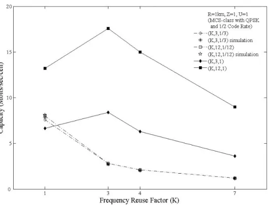
The system capacity for different frequency reuse factors with only one MCS-class (MCS-class with QPSK) and no reuse partitioning are shown as in Figure 5. Fundamentally, the system capacity is limited by two dominant factors. One is the number of available channels in a sector (beam), the other is the intra- and/or

Table 1 OFDMA parameters used in numerical results

Parameter Value

Total Bandwidth 10 MHz

FFT size 1024

OFDM symbol duration (including cyclic-prefix), T_OFDM 102.9 μs Cyclic-prefix 11.4μs

Sub-carrier frequency spacing 10.94 kHz

Number of sub-channels, N C 216

Number of sub-carriers in a sub-channel, N _S 4 Number of sub-carriers for data transmission 864 Number of sub-carriers for guard band 160 (1024-864)

Frame duration, Tframe 5ms

inter-cell interference. For a fixed antenna configuration, different reuse factors K and (channel) reuse patterns make a tradeoff between these two factors. Apparently, as seen in the figure, for the no-reuse case, the dominating limit factor is the number of available channels and therefore increasing K reduces the system capacity, although the inter-cell interference is reduced at the same time. For the full-reuse case, however, the intra-and/or inter-cell interference plays a more prominent role in determining the system capacity because the number of available channels has been increased by channel reuse. In this case, as is seen, K =3 provides the best tradeoff between the

capacity for both the 3-sector and switched-beam smart antennas. In addition, switched-beam smart antenna provides a significant gain over 3-sector antenna in full-reuse case because of more frequent channel reuse and larger antenna gain. Note that the performance of cell architecture

(

{ }

1 ,3,1

)

is worse than that of

(

{ }

1 ,3,1/ 3

)

because of too large intra- and/or inter-cell interference for usingK = . In the figure, 1 it is also shown that simulation results match well with the numerical results; the difference is within 1.3% ~ 3.9%.

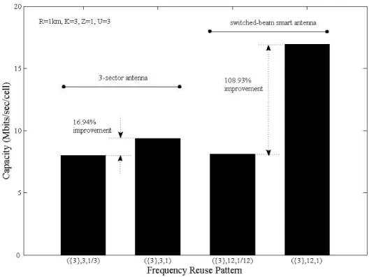
Figure 6 shows the system capacity for different channel reuse patterns and antenna configurations with 3 MCS-classes. Recall that K =3 provides the highest

system capacity. Again, for multiple MCS-classes, employing full channel reuse improves the system capacity. The improvement is more significant for switched-beam smart antenna because of much less inter-cell interference.

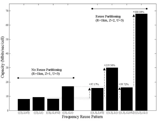
In Figure 7, the capacity improvement by using fractional frequency reuse is investigated. The results in the left side are reproduced from Figure 6 for comparison purpose. It shows that the capacity is substantially improved (97.1 - 300%) by applying reuse partitioning cell structure. Comparing the cases of

(

{ }

3 ,12,1

)

with

{ }

(

1,3 ,12,1

)

, the improvement by reuse partitioning is very significant by intra-cell frequency reuse. It is because in the inner cell the MCS-class with 64QAM is almost employed exclusively throughout all the beams because low inter-cell interference.

Chapter 3

An Improved Fast Base Station Switching

Technique for Cellular OFDMA Systems

Fast base station switching (FBSS) is an important handover mechanism in the orthogonal frequency division multiple access (OFDMA) mobile cellular systems. By employing one radio connection and multiple network connections during handover, FBSS strikes a good balance between complexity and handover performance, as compared to hard handover and macro diversity handover. In Section 3.1, the FBSS defined in IEEE 802.16 standard is first overviewed. Then, an improved FBSS with reuse partitioning is proposed in Section 3.2 to improve the performance of the traditional FBSS in OFDMA mobile cellular systems.

3.1 Fast Base Station Switching in IEEE 802.16 Network

There are three kinds of handover defined in IEEE 802.16e: hard handover, macro diversity handover (MDHO) and fast base station switching (FBSS). In hard handover, the system maintains only one connection in both the network and radio-link sections for the MS (mobile station), and therefore the network and radio-link connections to the target base station (BS) will be established only after breaking the existing ones. Hard handover is very simple, but services will be disrupted for a period of time needed for the establishment of the new connections. Contrary to hard handover, the system maintains multiple network and radio-link connections at the same time for the MS in MDHO. Therefore, both the network and radio-link connections to the target

essentially a soft handover, the service disruption can be eliminated by having multiple network and radio-link connections simultaneously. MDHO needs more than one receiver in the MS and hence increases its complexity. In addition, two copies of radio resource are needed for handover users and that leads to lower system spectrum efficiency and higher downlink interference.

FBSS, on the other hand, takes advantage of the low service disruption time from MDHO and low MS complexity from hard handover [8,25]. At network section, FBSS establishes connections with potential target BSs before breaking the existing one, so that the service disruption time can be reduced like in MDHO. Meanwhile, only one connection will be maintained at the radio-link section so as to keep low MS complexity as in hard handover. By switching between BSs fast enough, the MS can maintain its link performance and explore macro diversity gain.

In FBSS, the radio-link will not be switched to the target BS before the establishment of the new network connection to the target BS; otherwise, packets might be lost and/or become obsolete. This is especially important for real-time services. Unfortunately, the time needed for the establishment of a network connection is uncertain (a random variable) and cannot be known in advance [26]; to initiate the establishment of network connection too early will waste the network resource, but too late the radio-link performance might be degraded to an unacceptable level and that incurs packet loss.

In this section, an improved FBSS with reuse petitioning (RP) cell structure is proposed for IEEE 802.16e. By reserving some of the radio resource for use of high reuse factor, and using that radio resource to accommodate those handover users with bad radio-link performance, the packet loss rate can be substantially reduced, at the slight expense on average cell throughput.

3.1.1 Fast Base Station Switching in IEEE 802.16e

In the IEEE 802.16e system, an FBSS handover begins with a decision for an MS to transmit/receive data to/from the Anchor BS that may change within the diversity set [8]. Diversity set is a set containing a list of active BSs that are informed of the MS capabilities, security parameters, service flows and full MAC context information, and the Anchor BS is the BS in the diversity set that is designated to transmit/receive data to/from the MS at a given frame. Based on the received signal quality, the MS in FBSS handover can fast switch the Anchor BS so as to obtain the macro diversity gain. For good performance, the MS can scan the neighbor BSs and select those suitable ones to be included in the diversity set (diversity set selection/update), and the MS shall select the best BS from its current diversity set to be the Anchor BS (Anchor BS selection/update) [8].

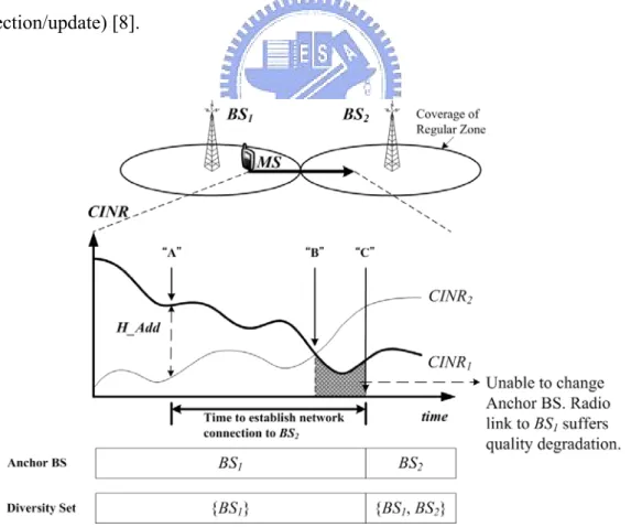
Figure 8. Cell structure, received radio-link signals, diversity set membership and Anchor BS selection of an MS involved in FBSS in IEEE 802.16e.

Figure 9. The message flow of FBSS in IEEE 802.16e

Figures 8 and 9 are used to explain the FBSS operation in IEEE 802.16e in details. For simplicity only two BSs are considered. Assume the MS is moving from BS1

toward BS , and 2 BS1 is the Anchor BS at the beginning. In IEEE 802.16e, the

parameter H Add₋ , a threshold used to trigger diversity set selection/update, is broadcasted through DCD (Downlink Channel Descriptor), and the characteristics of neighbor BSs (BS in this case) including BSID, PHY Profile ID, Preamble Index, ₂

etc. through the MOB_NBR-ADV message. Base on the information, the MS may send MOB_SCN-REQ to BS₁ and get response from MOB_SCN-RSP for requesting

of BS , as shown in Figure 9. When the CINR (Carrier to Interference plus Noise ₂

Ratio) difference of BS₁ and BS is less than H Add_{2 −} , the MS sends

MOB_MSHO-REQ with a recommended BS list including BS . If ₂ BS is also in ₂

the recommended list in MOB_BSHO-RSP, which is replied by BS₁, then the MS

sends MOB_HO-IND to request to add BS to the diversity set, i.e., to initiate the ₂

diversity selection/update procedure. In Figure 8, this first happens at the time instant A. After that, BS₁ sends HO-Request to BS through wire-line network to establish ₂

the network connection, and BS will reply HO-Response to ₂ BS₁ if the

establishment is complete. Accordingly, BS₁ can update the MS new diversity set

members through MOB_BSHO-RSP. When the MS keeps moving and if

2

CINRBS is higher than CINRBS1, for example

at the time instant B in Figure 8, the MS may send MOB_MSHO-REQ to request to change Anchor BS from BS₁ to BS (initiation of the Anchor BS selection/update ₂

procedure). The request, however, will not be granted in this example until the time instant C because the network connection to BS is not yet established (for some ₂

reason) before that instant, and BS will not be included in the diversity set. If the ₂

request is granted, through MOB_BSHO-RSP, the MS will send MOB_HO-IND to terminate the existing radio link connection and then perform fast ranging withBS , ₂

see Figure 9. Note that BS needs to reserve an uplink contention-free ranging ₂

sub-channel for the MS and to place Fast_Ranging_IE in the extended UIUC (Uplink Interval Usage Code) in a UL-MAP IE (Information Element) to inform the MS this ranging opportunity. The fast ranging process can be accomplished in two frames, where the uplink ranging opportunity is indicated by the downlink MAP in the first downlink sub-frame, and then the MS sends RNG-REQ in the successive uplink sub-frame based on the radio parameters recorded in the scanning interval. Then

replies RNG-RSP along with the correction commends encoded in TLV formats in the second frame. After that, the MS begins to transmit/receive data to/fromBS . ₂

As is mentioned, the MS is not able to change its Anchor BS to BS until the time ₂

instant C, although

2

CINR_BS is already higher than

1

CINR_BS at the time instant B. During the time period between B and C, the MS still talks toBS but with a ₁

degraded link performance, and that may result in packet loss. One simple remedy to this problem is to use a larger H Add₋ ; in other words, the request for diversity set update is initiated earlier. This, however, may waste network resource if BS is put ₂

into the diversity set too early. In the next section, an FBSS with reuse partitioning cell structure is proposed to improve the handover performance at the expense of slight loss in average cell throughput.

3.2 An Improved Fast Base Station Switching Technique for

Cellular OFDMA Systems

Reuse partitioning (RP) is a cell structure in which a regular cell is divided (ideally) into two or more concentric cell-regions, each with a different frequency reuse factor as introduced in section 2.1.1. This also implies that the radio resource of a cell has to be divided into the same number of resource-regions. A smaller reuse factor (small reuse distance) is allowed for the inner cell-regions because of the smaller transmit power, and a larger reuse factor is needed for the outer cell-regions so as to maintain the required signal quality. By allowing the inner regions to use a smaller reuse factor leads to a higher system capacity, as compared to the regular cell structure where the same reuse factor is used for the entire cell [19]. In this section, the concept of reuse partitioning is used to increase the handover performance.

3.2.1 Reuse Partitioning in IEEE 802.16e

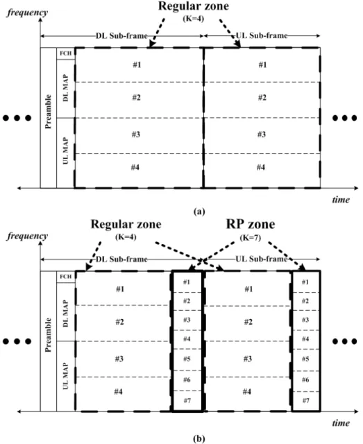
Figure 10(a) shows a simplified TDD frame structure in IEEE 802.16e. Preamble, FCH (Frame Control Header), downlink MAP and uplink MAP are control signals of the frame. It can be treated as an example of the frame structure depicted in Figure 4(a). The cell-specific Preamble is mainly used for downlink synchronization. FCH contains DL_Frame_Prefix that indicates the length and coding scheme of the DL_MAP message. DL_MAP and UL_MAP are MAC messages that define the starting point of the downlink and uplink bursts, respectively.

In IEEE 802.16e, frequency reuse with factor K can be achieved by dividing the radio resource in a frame into K resource-regions and each one of them is allocated to different BS. In Figure 10(a), K is equal to 4 so that the radio resource (both downlink and uplink) is divided into 4 resource-regions. Note that BSs need to be

synchronized and follow the same sub-carrier permutation rule for this scheme to work.

In order to design a reuse partitioning scheme, we adopt the concept of resource zone in IEEE 802.16e [8]. As an example, in addition to the regular resource-zone for

4

K = , a reuse partitioning (RP) zone is defined for K =7, as shown in Figure 10(b).

Again, within each respective zone, the radio resource is divided into K resource-regions and each one of them is allotted to different BS.

3.2.2 FBSS with Reuse Partitioning

The concept of reuse partitioning is used here to increase the performance of FBSS handover. The basic idea is as follows. Under the reuse partitioning cell structure, the handover users who are in a bad channel condition are scheduled to a resource-region with a large reuse factor so that a better CINR can be maintained, and therefore the packet loss rate is reduced. This method is very effective for the handover users who are waiting for the target BS to establish the network connection, as discussed in the previous section.

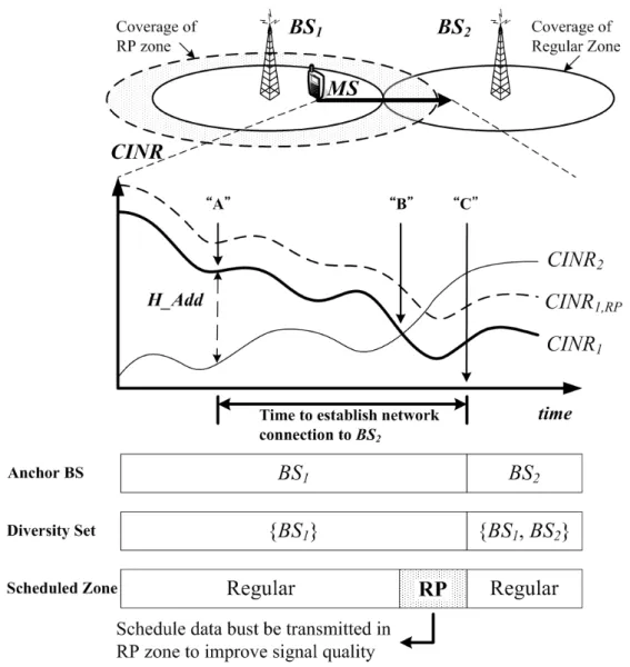
Figure 11 shows the RP cell structure and the received radio-link signals, diversity set membership and Anchor BS of an MS involved in FBSS. K = for the inner 4 cell-region and K =7 for the outer one with the resource-regions given in Figure

10(b). In the K =7 resource-region, since a large reuse factor is used, the received

CINR of an MS is higher as compared to the K = resource-region. Initially, the 4 MS talks to BS by using resource in the ₁ K = resource-region. As discussed in 4

the previous section, during the time between B and C, although

2

CINRBS is higher

than CINRBS₁, the MS still talks to BS since the network connection to 1 BS is not 2

ready yet. In the case of using reuse partitioning, the difference from Figure 8 is that now we have K =7 resource-zone, and the handover users going through this period

of time can be re-scheduled to that region to improve the radio-link performance if its CINR is less than the threshold ρ_req. Therefore, the packet loss during this period will be mitigated and the packet loss rate can be substantially reduced.

Figure 11. Reuse partitioning cell structure, received radio-link signals, diversity membership, Anchor BS selection and scheduled zones of an MS in FBSS with reuse

3.2.3 Simulation Results

In this section, simulation results are given to illustrate the handover performance of FBSS with and without reuse partitioning.

A. Simulation Model

The IEEE 802.16e downlink OFDMA system is simulated in a multi-cell urban environment, where cells are assumed to be synchronized to each other. Total of 19 cells is simulated with 1 km cell coverage under 15 Watts transmit power. K =4 for

the regular resource-zone and K =7 for the RP resource-zone. Each cell has three

sectors. The OFDM PHY parameters are given in Table 2.

At the beginning of the simulation, MSs are generated by Poisson processes and located randomly in a cell. The path loss to every BS is calculated for each MS, and the log-normal shadow fading (with de-correlation distance of 50m) and frequency-selective fading are generated according to the models given in [27]. An MS will send a service request to the BS with the highest effective SINR, and the request will be granted if there is radio resource available. Otherwise, the MS will be blocked and removed in the simulator. The effective CINR is evaluated on the received preamble signal part by the EESM (Exponential Effective SIR Mapping) criterion [28]. The location of an MS is periodically updated based on ITU vehicular mobility model [29] with mobility of 50km/hr. According to the mechanism proposed in section 3.2.2, the diversity set of an MS may be updated according to the CINR variation. Moreover, the anchor BS is the BS in diversity set with the highest CINR, and the MS only transmits/receives the radio signal to/from the anchor BS.

The G.729 VoIP traffic model is adopted in the simulation. The VoIP packet arrives every 20 ms with a packet size of 640 bits. The packet error rate is determined by the received SINR of the data traffic part and can be obtained by looking up table given in

Table 2 Parameters for system-level simulation

Parameter Value

Channel bandwidth 6 MHz

FFT size 2048

OFDM symbol duration (including cyclic-prefix)

336μs

Cyclic-prefix 37.333μs Sub-carrier frequency spacing 3.348 kHz

Frame duration 20ms

Downlink sub-frame duration 10ms

Sub-carrier permutation rule Adjacent sub-carrier permutation

Number of bins 192

Number of sub-carriers in a bin 9 Number of sub-carriers for data transmission 1728

Number of sub-carriers for guard band 320 (2048-1728)

Sub-channel definition 2 adjacent bins × 3 adjacent symbols

Maximum diversity set size 3

Threshold to schedule MS into the RP zone _{6 dB (}

req

ρ )

Time to establish network connection Uniform distributed between 200ms~700ms [26]

B. Simulation Results

The performances of FBSS are given in Figure 12, where P is the percentage of _RP

radio resource allotted to the K = resource-region. Three sets of results are given 7 including packet loss rate, average diversity set size and cell throughput. In all of the results P_RP = represents the case of traditional FBSS; that implies no RP 0 resource-region is reserved. Figure 12(a) shows the result of packet loss rate. As can be seen, P should be large enough, says more than 5%, in order to obtain a sizable RP

reduction on packet loss rate. More specifically, 38.33% to 84.08% reductions are achievable by increasing P from 7.29% to 21.88%, with respect to the

case P_RP = . Note that the packet loss rate reduction becomes saturated if 0 P is _RP

larger than around 21.88%. In addition, for a P_RP, a lower packet loss rate is obtained

with a larger H Add₋ .

Figure 12(b) shows the average diversity set size, which is an indicator on the network resource usage. As expected, the diversity set size is unchanged with different PRP for a specific H Add− . On the other hand, when increasing H Add− ,

the neighbor BSs might be added to the diversity set too early before the MS really needs to change its Anchor BS. Therefore the average diversity set size is larger and more network resource is consumed.

The cell throughput is shown in Figure 12(c). Since frequency reuse factor is larger in RP zone, the larger PRP, the lower the cell throughput. The results show that less

than 4.21% cell throughput will be lost even when P is increased to 21.88%. It is _RP

because the reduction on packet loss rate can increase the effective packets received by the MS, which can increase the cell throughput.

In summary, the performance tradeoff can be investigated by Figure 13, which is translated from Figure 12(a) and Figure 12(c). By reserving some of the radio resource for high reuse factor, and using that radio resource to accommodate handover users with bad radio-link performance, Figure 13 shows that the packet loss rate of FBSS is significantly reduced at a slight expense of cell throughput.