Contents lists available atScienceDirect
Computer Physics Communications
journal homepage:www.elsevier.com/locate/cpcA true-direction reconstruction of the quiet direct simulation method
for inviscid gas flows
Y.-J. Lin
a, M.R. Smith
b,c, F.-A. Kuo
a,c, H.M. Cave
a,d, J.-C. Huang
e, J.-S. Wu
a,∗aDepartment of Mechanical Engineering, National Chiao Tung University, Hsinchu, Taiwan bDepartment of Mechanical Engineering, National Cheng Kung University, Tainan, Taiwan cNational Center for High-performance Computing, Hsinchu, Taiwan
dDepartment of Mechanical Engineering, University of Canterbury, Christchurch, New Zealand eDepartment of Merchant Marine, National Taiwan Ocean University, Keelung, Taiwan
a r t i c l e i n f o
Article history:
Received 1 December 2012 Received in revised form 4 April 2013
Accepted 8 May 2013 Available online 20 May 2013
Keywords: QDSMC QDS Euler equations TDEFM CFD
Kinetic theory of gases
a b s t r a c t
In this paper, a true-direction flux reconstruction of the second-order quiet direct simulation (QDS-2N) Smith et al. (2009) [3] as an equivalent Euler equation solver, called QDS-N2, is proposed. Because
of the true-directional nature of QDS, where volume-to-volume (true-direction) fluxes are computed, as opposed to fluxes at cell interfaces as employed by traditional finite volume schemes, a volumetric reconstruction is required to reach a totally true-direction scheme. The conserved quantities are permitted to vary (according to a polynomial expression) across all simulated dimensions. Prior to the flux computation, QDS particles are introduced using properties based on weighted moments taken over the polynomial reconstruction of the conserved quantity fields. The resulting flux expressions are shown to exactly reproduce the existing second-order extension for a one-dimensional flow, while providing a means for true multi-dimensional reconstruction. The new reconstruction is demonstrated in several verification studies. These include a shock–bubble interaction problem, an Euler-four-shock interaction problem, and the advection of a vortical disturbance. These results are presented, and the increased computation time and the effect of higher-order extension are discussed in this paper. The results show that the proposed multi-dimensional reconstruction provides a significant increase in the accuracy of the solution. We show that, despite the increase in the computational expense, the computational speed of the proposed QDS-N2method is several times higher than that of the previously proposed QDS-2N scheme for
a fixed degree of numerical accuracy, at least, for the test problem of the advection of vertical disturbances. © 2013 Published by Elsevier B.V.
1. Introduction
There are a number of approaches for the simulation of gas flows, depending on the nature and level of rarefaction of the flow. Computational fluid dynamics (CFD) typically uses the finite volume method to solve a set of discretized governing equations, usually the Euler or Navier–Stokes equations for continuum flows. Contemporary finite-volume CFD divides the computational domain into a grid of cells, and fluxes of mass, momentum, and energy are calculated through the interfaces between these cells. This technique may suffer from the major disadvantage that the poor alignment of the grid with the flow field may result in large errors for some important flows (e.g., explosive blast wave), since fluxes can only occur between cells that share an interface, i.e., no reflection of the true-direction nature of the gas flow. Thus,
∗Corresponding author. Tel.: +886 3 573 1693; fax: +886 3 611 0023. E-mail address:[email protected](J.-S. Wu).
CFD requires a careful grid design to ensure accurate results, convergence, and stability.
Since the development of direct simulation Monte Carlo (DSMC) by Bird [1] for statistically solving the Boltzmann equation, a large number of continuum kinetic theory-based schemes have emerged following a similar spirit. In 1980, Pullin [2] proposed the equilibrium flux method (EFM) as an analytical equivalent to the equilibrium particle simulation method (EPSM), which is a di-rect simulation method where particles are forced to assume the Maxwell–Boltzmann equilibrium velocity probability distribution function instead of performing collisions. Later, Smith et al. [3] proposed a general form of the EFM method known as the true-direction equilibrium flux method (TDEFM), which captures rel-atively accurately the transport mechanism employed by EPSM. Fluxes calculated by TDEFM represent the true analytical solution to the molecular free flight problem, under the assumptions of thermal equilibrium and uniformly distributed quantities in each cell.
0010-4655/$ – see front matter©2013 Published by Elsevier B.V.
Y.-J. Lin et al. / Computer Physics Communications 184 (2013) 2378–2390 2379
Albright et al. [4] developed a numerical scheme for the solution of the Euler equations, known as the quiet direct simulation Monte Carlo (QDSMC) method. In this method, the integrals encountered in the TDEFM formulation are replaced by approximations using Gaussian numerical integration, effectively replacing the continu-ous velocity distribution function with a series of discrete veloc-ities. The method was later renamed the quiet direct simulation (QDS) method, because of the lack of stochastic processes, and was extended to second-order spatial accuracy [5]. The lack of complex mathematical functions results in a computationally very efficient scheme with a considerably higher performance than EFM while maintaining the advantages of true-directional fluxes like TDEFM. Because of the assumption of unrestricted motion during free flight, each of the abovementioned kinetic solvers has a large amount of (cell-size-based) numerical diffusion. To combat this dissipation, a common strategy, employed in conventional finite volume methods, is to apply the higher-order reconstruction of properties or fluxes. Macrossan [6] applied EFM using higher-order spatial extensions, while Smith [7] attempted the analytical in-clusion of gradients into true-direction volume-to-volume fluxes, only to find that the complete analytical inclusion of gradient terms in the TDEFM flux expressions is impossible. Smith et al. [5] re-duced the numerical diffusion by applying ‘‘simplified’’ flux recon-struction at the interface that improves the original QDS to be almost second order in spatial accuracy; this method is called QDS-2N.
In this paper, we extend the second-order QDS algorithm (QDS-2N) [5] to higher-order reconstruction through the true-direction polynomial multi-dimensional reconstruction of conserved prop-erties across each cell width; this method is called QDS-N2. The net fluxes are computed through the individual contributions of QDS particles, computed by taking moments over the polynomial reconstruction. The particle properties are updated, considering the average value of the conserved quantity between the region bounds, which are required in translational directions and the application of splitting. The fluxes of conserved properties are cal-culated by a sum of weighted moments over the polynomial spa-tial reconstruction of mass, momentum, and energy across the cell width. The verification simulations of four two-dimensional cases are carried out to show the improved accuracy of the proposed QDS-N2scheme for inviscid gas flow simulations.
2. Numerical method
2.1. Quiet direct simulation (QDS)
The normal random variable N
(
0,
1)
is defined by the probabil-ity densprobabil-ity:p
(
x) =
e−x2/2
√
2
π
.
(1)By using a Gaussian quadrature approximation, the integral of Eq.(1)over its limits can be approximated by:
∞ −∞ e−x2/2√
2π
f(
x)
dx≈
N
j=1w
jf(
qj)
(2)where
w
j and qjare the weights and abscissas of the Gaussianquadrature (also known as the Gauss–Hermite parameters), and N is the number of terms. The abscissas are the roots of the Hermite polynomials, which can be defined by the recurrence equation:
Hn+1
(
q) =
2qHn−
2nHn−1 (3)where H−1
=
0, and H0=
1. The weights can be determined from:w
j=
2n−1n
!
√
π
n2[H
n−1
(
qi)
]2.
(4)The net fluxes of mass, momentum and energy of a cell are given by the sum of individual flux contributions from all the particles flowing in and out as follows:
FMASS
=
M
J=1 FMASSJ
in−
N
J=1 FMASSJ
out,
FMOM=
M
J=1 FMOMJ
in−
N
J=1 FMOMJ
out,
FENG=
M
J=1 FENGJ
in−
N
J=1 FENGJ
out (5)where FMASSJ , FMOMJ and FENGJ is the individual mass flux, individual momentum flux and individual energy flux from particle J respec-tively, M and N is the number of inflow and outflow particles re-spectively into the cell under consideration. Each of the individual contributions (with first order spatial accuracy) can be described by the expressions, e.g., in one-dimensional case:
FMASSJ
=
v
J∆t ∆x mJ F J MOM=
v
J∆t ∆x mJv
J FENGJ=
v
J∆t ∆x mJ
1 2v
2 J+
ε
J
(6)where the particle mass mJ, particle velocity
v
J, and particleinter-nal energy
ε
Jare expressed as:mJ
=
ρ
∆ xw
J√
π
v
J=
u+
√
2σ
qJε
J=
(ξ −
Ω) σ
2 2 (7)where
ρ
is the density, u is the bulk (or mean) flow velocity, andσ = (
RT)
1/2in a given source cell. Note R is the universal gas con-stant, and T is the gas temperature. The total number of degrees of freedomξ
is defined asξ =
2(γ −
1)
−1whereγ
is the specific heat ratio(=
Cp/
Cv)
, andΩ is the number of simulated degreesof freedom (e.g.,Ω
=
1 for one dimensional flow). In the exist-ing QDS-2N [5], the values ofρ,
u, andσ
employed in QDS particle initialization are taken from reconstructions based on linear vari-ations between neighbor cells. Despite fluxes being true direction in nature, the reconstructions performed in previous implementa-tions are directionally decoupled—i.e. a flux is computed through the product of (separate) fluxes previously computed (for 2D flow) in the x and y directions. For the 2D case, the particle mass and ve-locities in Eq.(7)become:mJK
=
ρ
∆x∆yw
Jw
Kπ
v
J=
ux+
√
2σ
2q Jv
K=
uy+
√
2σ
2q K (8) where there are K=
1, . . . ,
M particles in the y-direction and thedefinition of other variables are the same as those in 1D case. The internal energy remains identical to the 1-D case, allowing for a corresponding increase inΩ to account for the extra simulated dimension. The fluxes from sources cell to any arbitrary destina-tion cell can be calculated by the particle posidestina-tion distribudestina-tions. The fluxes of mass, momentum and energy, which are based on the proportion of the overlapped area to the area of the original cell, are given by:
FMASS
=
A As mJK FMOM−X=
A As mJKv
J FMOM−Y=
A As mJKv
K FENG=
A As mJK
1 2(v
2 J+
v
2 K) + ε
JK
(9)Fig. 1. The special reconstruction convention for current amount of conserved quantity Q in one cell.
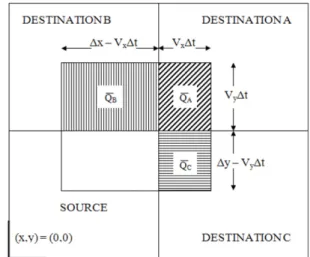
Fig. 2. QDS flux procedure within a general (arbitrary) special reconstruction of conserved quantity Q .
where A is the overlapped area as u
·
v ·
dt2and Asis the source cell
area as dx
·
dy.2.2. Spatial reconstruction and flux calculation
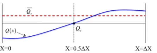
In the current study, referring toFig. 1, the general extension to higher order in QDS in one-dimensional case is performed using a spatial reconstruction of the form:
Q
(
x) =
Qc+
dQ dx
x=0.5∆x(
x−
0.
5∆x)
+
d2Q dx2
x=0.5∆x(
x−
0.
5∆x)
2 2+ · · · +
dn−1Q dxn−1
x=0.5∆x(
x−
0.
5∆x)
n−1(
n−
1)!
(10)where Q
(
x)
is the value of a conserved property (mass, momen-tum, or energy) at a distance x from the left hand side of the cell, and integer n indicates the order of the reconstruction. Note Qcis the value of Q
(
x)
at the cell center. This value is calculated from Q(
x)
integrating over the cell width divided by the cell width equaling to the existing average value of the source cell Qs,pre-sented below: Qs
=
1 XR−
XL
XR XL Q(
x)
dx=
Qcx+
1 2
dQ dx
(
x−
0.
5∆x)
2+
1 6
d2Q dx
(
x−
0.
5∆x)
3+ · · ·
x=XR x=XL.
(11)By using our revised reconstruction, the bounds of integration are XL
=
0 and XR=
∆x. Then, Eq.(11)leads to:Qs
=
Qc+
∆x2 24
d2Q dx2
+
∆x 4 1920
d4Q dx4
+ · · · +
2∆x n−1 n!
1 2
n
dn−1Q dxn−1
.
(12)Alternatively, Qccan be expressed as follows: Qc
=
Qs−
∆x2 24
d2Q dx2
−
∆x 4 1920
d4Q dx4
− · · · −
2∆x n−1 n!
1 2
n
dn−1Q dxn−1
(13) where n is assumed to be an odd number. This shows that the cor-rection is only required when the scheme is third order (n=
3) accurate or higher, otherwise Qc=
Qs(e.g., n=
2). Thus, thecom-plete correct form of the higher order reconstruction of Q
(
x)
usingQscontains additional terms on every even derivative: Q
(
x) =
Qs−
∆x2 24
d2Q dx2
−
∆x 4 1920
d4Q dx4
+
dQ dx
(
x−
0.
5∆x) +
d2Q dx2
(
x−
0.
5∆x)
2 2!+
1 3!
d3Q dx3
(
x−
0.
5∆x)
3+
dnQ dxn
(
x−
0.
5∆x)
n n!
.
(14)Specifically, as n
=
2, the above is reduced to the following form because of Qc=
Qs, as shown below:Q
(
x) =
Qs+
dQ dx(
x−
0.
5∆x) +
1 2! d2Q dx2(
x−
0.
5∆x)
2.
(15)The above reduces to exactly the same form as in QDS-2N [5]. Next, referring to Fig. 2, the outgoing flux value of average conserved quantity successfully moving from the source cell into the destination cell (denoted by Qtr) is:
Qtr
=
1(
XR−
XL)
XR XL Q(
x)
dx=
1(
XR−
XL)
Qcx+
1 2
dQ dx
×
(
x−
0.
5∆x)
2+ · · ·
x=∆x x=∆x−u∆t=
Qc+
1(
XR−
XL)
1 2
dQ dx
×
(
x−
0.
5∆x)
2+ · · ·
x=∆x x=∆x−u∆t (16) where the bounds of integration are XL=
∆x−
u∆t and XR=
∆x.Now, the transition of mean values Qtrcan be used to calculate
particle properties. Assigning the flux out of average conserved properties Q1tr
,
Q2trand Q3tras the mass, momentum, and energy, respectively, the resulting QDS particle properties for particle J are:mJ
=
Q1trWJ√
π
,
v
J=
Q2tr Q1tr+
2R(
Cv)
2
Q3tr Q1tr−
1 2
Q2tr Q1tr
2
1 2 qJ,
ε
J=
(ξ −
Ω)
R 2
Q3tr Q1tr−
1 2
Q2tr Q1tr
2
.
(17)Y.-J. Lin et al. / Computer Physics Communications 184 (2013) 2378–2390 2381
Fig. 3. Flowchart describing QDS particle computation with gradient inclusion.
To calculate the average value of conserved property for higher order reconstruction, it is important how the flux limiting is cou-pled. According to the value of conserved property Q
(
x)
(see Eq.(10)), the gradient of Qcis defined in flux limiting during thereconstruction process. In each cell, we employ the monotonized central difference (MC) limiter to the effective gradients of con-served properties, as described below:
dQ dx
=
dQ dx
Fφ (θ)
(18)φ (θ) =
max
0,
min
2,
θ +
1 2,
2θ
(19) whereφ
is the equivalent flux limiter and F is the gradient calcu-lated using forward differences. Theθ
is the ratio of the first order gradient calculated using forward and backward differences:θ =
dQ dx
B
dQ dx
−1 F.
(20)Therefore, an alternate representation of the variation of Q
(
x)
over space can be:Q
(
x) =
Qc+
dQ dx
Fφ(θ)
x=0.5∆x(
x−
0.
5∆x)
+
1 2
d2Q dx2
Fφ (θ)
(
x−
0.
5∆x)
2+ · · · +
1 n!
dnQ dxn
Fφ(θ)
x=0.5∆x(
x−
0.
5∆x)
n.
(21)Fig. 4. Two-dimensional motion of a single QDS particle showing ‘‘sub-particle’’ contributions.
2.3. 1D flux calculation and implementation
In QDS simulations, we require flux from a volume to another volume. Since fluxes are split, the quantities of the fluxes depend entirely on the region from which they originated. The flux calculation is described as a flowchart inFig. 3, and summarized briefly as follows:
1. The gradients of conserved properties Q are first calculated using standard finite difference approximations in each cell i. For example, for a 5th order accurate reconstruction, one might use the
Fig. 5. Initial conditions of shock–bubble interaction problem.
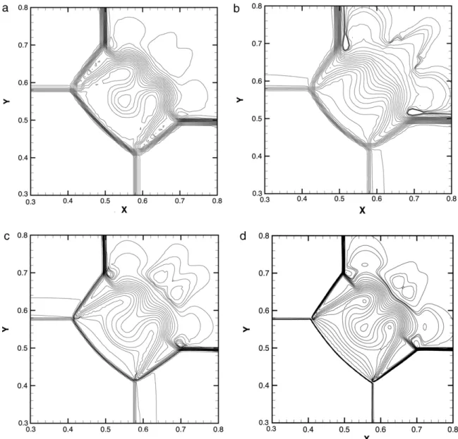
Fig. 6. Shock–bubble Schlieren image with 1700×500 cells at time of 0.2. QDS 2nd order (a) 2N scheme with van Leer’s limiter, (b) N2scheme, and (c) 2nd order TVD result
presented in [8] using the same resolution.
stencils like:
dQ dx
i=
Qi+1−
Qi−1 ∆x
d2Q dx2
i=
Qi+1+
Qi−1−
2Qi 2∆x
d3Q dx3
i=
1 ∆x2
dQ dx
i+1+
dQ dx
i−1−
dQ dx
i
(22)
d4Q dx4
i=
1 ∆x2
d2Q dx2
i+1+
d2Q dx2
i−1−
d2Q dx2
i
.
2. For each QDS particle:
a. Calculate the approximate particle velocity based on the current cell Qs, which should give the same particle velocity as 1st order QDS.
v
J=
Qs2 Qs1+
2R Cv2
Qs3 Qs1−
1 2
Qs2 Qs1
2
1 2 qJ.
(23)Y.-J. Lin et al. / Computer Physics Communications 184 (2013) 2378–2390 2383
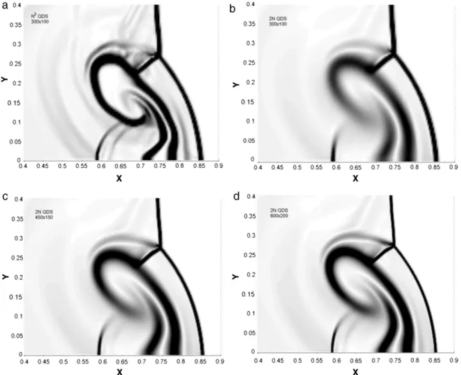
Fig. 7. Zoom of Schlieren image of shock–bubble problem at time 0.2; (a) QDS N2scheme with 300×100 cells; (b) QDS 2N scheme with 300×100 cells; (c) QDS 2N scheme
with 450×150 cells; (d) QDS 2N scheme with 600×200 cells.
Fig. 8. The initial conditions for the first problem of Euler-four-shock interaction.
b. Calculate the integral bounds XLand XR:
If V
>
0,
XR=
∆x−
u∆t XL=
∆x
,
otherwise
XR=
0 XL=
u∆t
.
(24)c. Calculate the flux out values of average conserved properties
Qtrof particles to successfully move into the destination region.
d. Calculate the particle properties based on the average values
Qtr.
e. Calculate the fluxes of conserved properties to neighboring cells following the standard QDS algorithm [5].
2.4. 2 D flux calculation and implementation
Multi-dimensional extension is performed using the same prin-ciple applied for a one-dimensional reconstruction. The variation of conserved quantity Q
(
x,
y)
over two dimensional space is as-sumed to be: Q(
x,
y) =
Qc+
dQ dx
x=0.5∆x(
x−
0.
5∆x)
+
d2Q dx2
x=0.5∆x(
x−
0.
5∆x)
2 2+ · · ·
+
dn−1Q dxn−1
x=0.5∆x(
x−
0.
5∆x)
n−1(
n−
1)!
+
dQ dy
y=0.5∆y(
y−
0.
5∆y)
+
d2Q dy2
y=0.5∆y(
y−
0.
5∆y)
2 2· · ·
+
dn−1Q dxn−1
y=0.5∆y(
y−
0.
5∆y)
n−1(
n−
1)!
.
(25)Fig. 9. Zoom of density contour line of Euler-four-shock problem. Comparing the second-order QDS N2solver (a) using 100×100 grids with MC limiter, (b) 2N solver using
100×100 grids, (c) 200×200 grids, and (d) 300×300 grids with MC limiter at time of 0.4.
The subsequent cell centered value of Qcis: Qc
=
Qs−
∆x2 24
d2Q dx2
−
∆x 4 1920
d4Q dx4
· · ·
−
2∆x n−1 n!
1 2
n
dn−1Q dxn−1
−
∆y 2 24
d2Q dy2
−
∆y 4 1920
d4Q dy4
· · ·
−
2∆y n−1 n!
1 2
n
dn−1Q dyn−1
.
(26)Following this, the average value of conserved quantity in the region bounded by
[
XL,
YB] − [
XR,
YT]
is formulated as:Qtr
=
1(
XR−
XL) (
YT−
YB)
YT YB
XR XL Q(
x,
y)
dxdy=
Qc+
1(
XR−
XL)
dQ dx
(
XR−
0.
5∆x)
2 2· · ·
+
dn−1Q dxn−1
(
XR−
0.
5∆x)
n n!
−
dQ dx
(
XL−
0.
5∆x)
2 2· · ·
+
dn−1Q dxn−1
(
XL−
0.
5∆x)
n n!
+
1(
YT−
YB)
dQ dy
(
YR−
0.
5∆y)
2 2· · ·
+
dn−1Q dyn−1
(
YR−
0.
5∆y)
n n!
−
dQ dy
(
YL−
0.
5∆y)
2 2· · ·
+
dn−1Q dyn−1
(
YL−
0.
5∆y)
n n!
(27) where YTand YBare the bounds of integration in y direction.Since the average requires bounding regions in both transla-tional directions, application of splitting (as applied to TDEFM to improve computational efficiency) is impossible, and the full QDS-N2number of particles (i.e. 9 when 3 particles are used per
Y.-J. Lin et al. / Computer Physics Communications 184 (2013) 2378–2390 2385
Fig. 10. Density contour lines of Euler-four-shock problem. (a) The 2nd order TVD–MUSCL∗scheme. (b) The third-order QDS N2scheme used 1000×1000 grids with MC
limiter at time of 0.8. (c) The third-order QDS 2N scheme used 1000×1000 grids with MC limiter.
∗
Source: Taken from Cada [8] using 1000×1000 points, CFL=0.8.
direction, 16 for 4, etc.) are required for a complete flux computa-tion. Previous extensions required only QDS-2N particles. Unlike the one-dimensional reconstruction, each particle carries three separate fluxes (for three different destination cells) and so any single QDS particle possesses three ‘‘sub-particles’’ based on differ-ent integral bounds. This concept is demonstrated inFig. 4, show-ing each unique sub-region (A–C). The area of the sub-region A is
u
·
v ·
dt2as described earlier in Section2.1for the QDS-2N method.3. Results and discussion
In this section, we present four test cases for comparing the QDS-N2and the QDS-2N schemes that are hereafter referred to as N2and 2N, respectively. These four test cases include shock–bubble interaction, Euler-four-shock interaction, Euler-four-contact in-teraction and advection of vortical disturbances. The major dis-cussions focus on the time cost and accuracy between the two schemes in two-dimensional problems.
3.1. Shock–bubble interaction
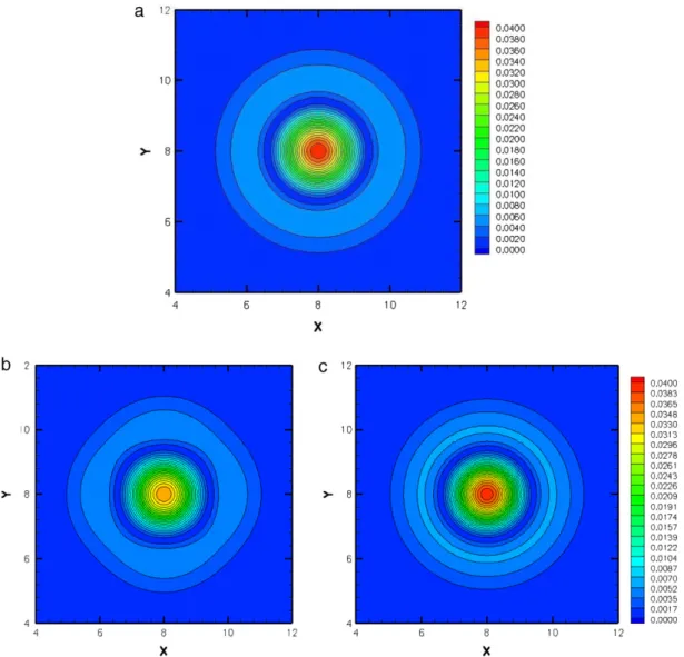
The strength of correct multi-dimension reconstruction is demonstrated in a two-dimensional shock/bubble interaction problem [8]. The initial conditions for this problem are shown in Fig. 5. The simulation calculates a shock wave, moving from left to right with a velocity of Mach number 2.85 in an ideal, inviscid gas and interacting with a bubble at x
=
0.
3. The results are pre-sented with the snapshot at t=
0.
2. The results of the numerical schlieren (gradients of density) are presented inFig. 6for various QDS schemes and the TVD scheme on a grid of 1700×
500 cells. The application of correct multi-dimensional reconstructions re-sults in a relatively high resolution of the circulation and reflected shock located at x=
0.
6.Fig. 7displays two QDS schemes with different numbers of cells. We compare the N2scheme with 300
×
100 cells (Fig. 7a) against the 2N scheme (Fig. 7b–d) by using 300×
100,
450×
150, and 600×
200 cells. For the sake of comparison, the limiter for each simulation is the monotonized central (MC) limiter. InFig. 7a and b, the difference in resolution is clear despite the fact that both theseFig. 11. The initial conditions for the second problem of Euler-four-contact interaction.
Fig. 12. Density profile of the four contacts problem for the second-order TVD– MUSCL method.
Source: Taken from [8] using 1000×1000 cells at time 0.8.
schemes employ the same number of cells. As the number of cells employed by the 2N scheme increases (shown up to 600
×
200 cells here), the results gradually approach those of the N2scheme with relatively few cells (1/
4). Obviously, the multi-dimensional computation (N2 scheme) achieves higher accuracy than the 2N scheme.Further, we consider the computation time required by each scheme in this case. The N2 scheme is true-directional, in that each possible combination of discrete velocity must be considered (nine instances with three discrete velocities per direction), while the 2N method employs approximate dimensional extension and only requires six discrete velocity computations in a two-dimensional simulation. Moreover, for each particle, three space-averaging computations are required for each fraction falling into separate destination cells. Therefore, the N2scheme requires more computation time for the same number of cells. The computation time of the two solvers are summarized in Table 1. According to these data, the N2 extension of QDS requires approximately three times the computation time as compared to that of the original 2N scheme for the same number of cells. However, for any given degree of accuracy, we find that the N2scheme provides an increase in computational efficiency of almost three times (300
×
100 vs. 600×
200 for 2N vs. N2). Thus, the application of the N2 scheme is justified over that of the 2N scheme for high-resolution solutions.Fig. 13. Density contour obtained from QDS N2solver (a) and 2N solver (b) by using
1000×1000 cells, 2nd order method with MINMOD limiter at a time of 0.8. The CFL number is 0.5. Level from 0 to 2.4 at 0.05 interval of line.
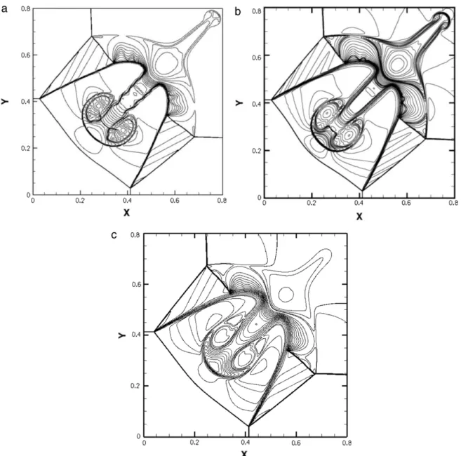
3.2. Euler-four-shock interaction
This test case was introduced in Salichs [9], which computed the numerical solution employing the piecewise hyperbolic method-Marquina’s flux formula (PHM-MFF) and power PHM-MFF schemes. The test problem is initially divided into four quadrants sharing a common corner at 0.75 and 0.75 in the domain
[0
,
1] ×[0
,
1], as illustrated inFig. 8. These quadrants initially have the following different but uniform conditions:(ρ,
u, υ,
p)
=
(
1.
5,
0,
0,
1.
5), [
0.
75,
1] × [0.
75,
1](A)(
0.
5323,
1.
206,
0,
0.
3),
[0
,
0.
75) × [
0.
75,
1](B)(
0.
138,
1.
206,
1.
206,
0.
029),
[0
,
0.
75) × [
0,
0.
75)
(C)(
0.
5323,
0,
1.
206,
0.
3),
[0
.
75,
1] × [0,
0.
75)
(D).
(28)Fig. 9shows four results of a comparison between the 2N and N2solvers at the time of 0.4. The Courant–Friedrichs–Lewy (CFL) factor is set as 0.5. We compare the results of the two QDS solvers using 100
×100 to 300
×
300 cells. As can be seen, the result of theY.-J. Lin et al. / Computer Physics Communications 184 (2013) 2378–2390 2387
Fig. 14. Density contour obtained from QDS-2N solver with 5 particles (a) and 9 particles in each direction (b); QDS-N2solver with 5 particles (c) and 9 particles in each
direction (d) by using 1000×1000 cells, 2nd order method with MINMOD limiter at time of 0.8. The CFL number is 0.5. Level from 0 to 2.1 at 0.05 interval of line.
Table 1
Comparison of computational expenses for QDS schemes using 2N and N2dimensional reconstruction.
Number of cells QDS scheme
2N (min) N2(min)
300×100 8.41 23.15
450×150 28.9 78.3
600×200 68.56 183.6
1000×500 478.4 1282.6
N2solver obtained using a coarse grid (100
×
100 cells) is only ap-proached by the 2N solver when employing considerably fine grids (300×
300 cells). Furthermore, the result that we obtained using the N2solver on a computational grid of 1000×1000 cells is similar to that obtained using the total variation diminishing–monotone upstream centered schemes for conservation laws (TVD–MUSCL) scheme [8] (seeFig. 10a).An investigation of the computational expense of each scheme showed that the N2solver takes approximately four times longer to complete the simulation than the 2N solver. This comparison of computational expense is summarized inTable 2. The increase in computational time with the refinement of the computational grid is due to the constant ‘‘kinetic’’ CFL condition that we employ,
Table 2
QDS scheme time cost in Euler-4-shocks interaction case. Number of cells QDS solvers
2N N2
1000×1000 13.29 h 55.6 h
100×100 45 (s) 189 (s)
200×200 375 (s) 1520 (s)
300×300 1307 (s) 5199 (s)
which is defined as follows:
CFL
=
Max
√
u2+
3∗
√
RT
∗
dt dx
,
√υ
2+
3∗
√
RT
∗
dt dy
.
(29)This basically ensures that particles in free flight do not travel further than the adjacent cells. Although the result takes more time to compute using the N2solver, the accuracy is considerably better than that of the 2N solver; in fact, it is not clear that the 2N
Fig. 15. Density contour obtained from QDS-N2solver using (a) 2000×2000 and
(b) 3000×3000 cells, 2nd order method with MINMOD limiter at time of 0.8. The CFL number is 0.5. Level from 0 to 2.1 at 0.05 interval of line.
solver will ever approach the solution obtained using the N2solver, irrespective of the number of cells employed.
3.3. Euler-four-contact interaction
This test case involves the Euler-four-contact interaction prob-lem defined by Schulz-Rinne, Collins, and Glaz [10]. The same test case with a different higher-order method is also presented in [11]. This Riemann problem briefly shows four constant states consist-ing of four quadrants and two shocks generated clockwise at the origin. The contact point is centered about the location
(
x,
y) =
(
0.
5,
0.
5)
. A representation of the initial conditions of the flow do-main is illustrated inFig. 11. The initial flow condition is imposed by four difference shock waves and satisfies the following relation:(ρ,
u, υ,
p) =
(
1,
0.
75, −
0.
5,
1),
[0
.
5,
1] × [0.
5,
1](A)(
2,
0.
75,
0.
5,
1),
[0
,
0.
5) × [
0.
5,
1](B)(
1, −
0.
75,
0.
5,
1),
[0
,
0.
5) × [
0,
0.
5)
(C)(
3, −
0.
75, −
0.
5,
1),
[0
.
5,
1] × [0,
0.
5)
(D).
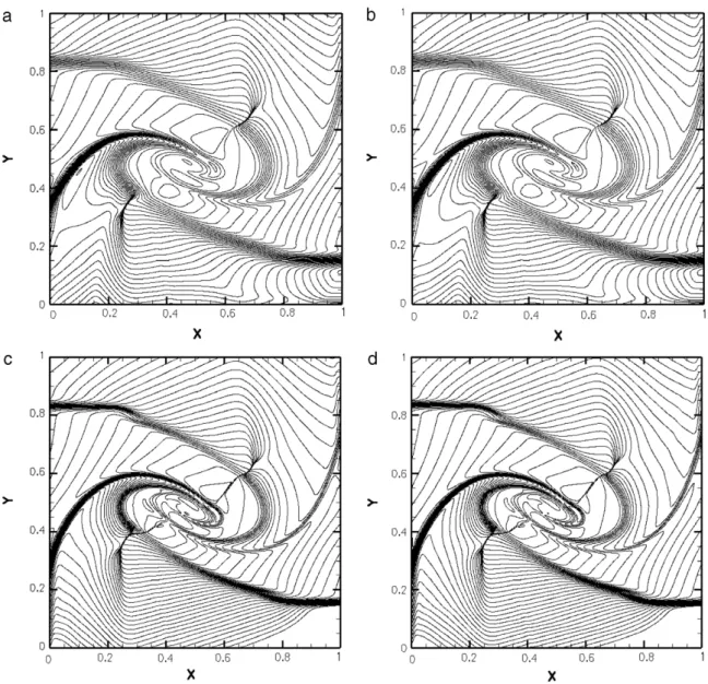
(30)Fig. 12 shows the numerical result of the second-order TVD–MUSCL method for a density contour profile on a 1000
×
1000 uniform grid, taken from [8]. For the QDS scheme, the result obtained at the time of 0.8 on a 1000×
1000 uniform grid can be seen inFig. 13. Two results are shown for the second-order method with the N2and the 2N solvers. Both enforce a constant CFL number of 0.25. The contours of density are presented with levels of 0–2.4. In this case, a shock wave is generated and spirals from the contact point in an unsteady fashion. By comparing the two figures, we find that both the N2and the 2N solver results are symmetrical and that the result obtained using the N2solver is closer to the TVD–MUSCL result presented inFig. 12. As in the previous test cases, in the current test case, the accuracy of the N2method is superior to that of the 2N method. In this instance, however, the essentially non-oscillatory weighted (WENO) results [11] are still superior to the N2results; this can be attributed to the small stencil employed for the estimation of the higher-order gradients or to the flux splitting employed and the inevitably associated numerical dissipation; this deserves further investigation.Further, we have compared the timings and the accuracy for this test problem with different N for both QDS-2N and QDS-N2with 1000×1000 cells since both schemes scale differently with N. The results are essentially the same as those obtained for N
=
3 whenN increases to 5 or 9 for both the abovementioned methods, as
shown inFig. 14. This is reasonable since the integration of a Gaus-sian function with a polynomial, having two or fewer degrees, be-comes exact, if the number of Gaussian–Hermite integration points is 3 or more. Expectedly, the computation time increases roughly 3 times from N
=
3 to N=
9 for both the methods. Further, Fig. 15shows the density contours when the grid resolution in-creases from 1000×
1000 cells to 2000×
2000 and 3000×
3000 cells. In brief summary, for both the QDS-2N and the QDS-N2 meth-ods for solving the Euler equation, accuracy effectively increases with increasing grid resolution, while it is essentially the same when N≥
3.3.4. Advection of vortical disturbance
The final test case consists of an inviscid unsteady flow in which a vortex is located at the center of a uniform domain
(
xc,
yc)
. Themean flow for this case uses Mach number M∞
=
0.
1. This casetests the capabilities of the QDS scheme as compared to the exact solution taken from Visbal and Gaitonde [12] in order to accurately advect vortical disturbances. This problem also appears in Tutkun and Edis [13]. The initial conditions are as follows:
u
=
U∞−
C(
y−
yc)
Rc2 exp−
r 2 2,
υ =
C(
x−
xc)
Rc2 exp−
r 2 2 p−
p∞=
ρ
C2 2Rc2 exp(
r2),
r2=
(
x−
xc)
2+
(
y−
y c)
2 Rc2 (31)where u,
υ
, and Rcdetermine the Cartesian velocity componentsand the vortex core radius, respectively. C is the vortex strength parameter, defined as follows:
C
(
U∞Rc)
=
0.
02.
(32)The density is assumed to be constant, and the vortex radius Rc
is taken to be 1.0 in this case.
Fig. 16shows the vorticity contours of the N2and the 2N solvers with 800×800 cells using the second-order method. The limiter in this case is the monotonized central (MC) method. A constant CFL number (0.1) is enforced such that the non-dimensional time step size is∆tU∞
/
Rc=
4.
0×
10−3. The result of the N2solver isessen-tially the same as the exact solution and shows a perfect circular shape of the vorticity distribution while that of the 2N solver does
Y.-J. Lin et al. / Computer Physics Communications 184 (2013) 2378–2390 2389
Fig. 16. Vorticity magnitude contours compared (a) exact solution and two result using 2nd order (b) QDS 2N solver and (c) QDS N2in 800×800 uniform cells. All results
are taken from CFL number to 0.1.
not. The result of the 2N solver shows more significant dissipation and anisotropy errors as compared to that of the N2solver.Fig. 17 shows the vorticity distributions of various simulations along a horizontal line (at y
=
8.
0) passing through the vortex center in Fig. 16. We have compared the results obtained by using the two solvers (2N and N2) on a uniform grid containing three different levels of resolution (160×160,
800×
800, and 1600×
1600 cells). The result obtained using the N2solver in the case of 800×800 cells is in excellent agreement with the exact solution and radial sym-metry, while the results obtained using the 2N solver are far from the correct solution even in the case of 1600×1600 cells. Thus, the
influence of multi-dimensional reconstruction is significant for the QDS, particularly on the numerical accuracy of the solution for a gas flow field as in the current problem.The investigation of the computational expense again reveals a trade-off between computational time and accuracy. The computa-tional time of the N2solver in terms of calculation time is approxi-mately 3∼4 times less than that of the 2N solver for the same computational grid, although the accuracy of the former is con-siderably better than that of the latter. This leads to a question of whether the use of the N2method is worthwhile or not. Thus, we compare the results obtained using the N2method using 160×160 cells with those obtained using the 2N method using 1600
×
1600 cells, as shown inFig. 17. The results show that they are essen-tially the same for the same level of accuracy; thus, the proposedN2 solver is approximately 25 times faster than the 2N solver in this case. Once again, we are unsure whether the 2N result will ever converge to the analytical solution, thereby justifying the ap-plication of the N2solver and its proposed multi-dimensional re-construction of QDS particles.
4. Conclusion
In this paper, a true-direction multi-dimensional higher-order extension of the QDS method, referred to as the N2solver, was in-troduced and verified using various test cases. The results showed that the N2 solver was considerably more accurate than the 2N solver in general. It appeared that the N2 solver (i) improved the solution in the flows unaligned with the computational grid and (ii) significantly reduced the amount of numerical dissipation within the solution. Despite the additional computational expense associated with the N2solver for the same computational grid, for any given degree of accuracy, the proposed solver was found to be several times (up to 25 times in the case of the advection of vorti-cal disturbances) faster than the original 2N method. Of particular interest was the test case of the advection of vortical disturbances, where the N2method improved the radial symmetry of the result approaching the analytical solution, while the 2N method failed to converge to the analytical solution even when a very fine grid
Fig. 17. The vorticity profiles along the central line passing through the vortex. The comparison contained the exact solution (blue squeal-symbol line), the QDS N2
solver using 160×160 cells (red line), 800×800 cells (black dash-dot line), and 2N solver using 800×800 cells (purple long-dash line), 1600×1600 cells (green dotted line). Two solvers are computed in the MC limiter and CFL=0.1 at time 8.0. (For interpretation of the references to colour in this figure legend, the reader is referred to the web version of this article.)
was used. In the cases of both the QDS-2N and QDS-N2methods for solving the Euler equation, accuracy effectively increases with increasing grid resolution, while it was essentially the same when
N
≥
3 because the integration of the Gauss function with a polyno-mial (degree≤
2) using the Gauss–Hermite integration technique became exact.A significant improvement on the errors associated with the flow misalignment with the computational grid was demon-strated through numerical experiments with the proposed multi-dimensional reconstruction employed by the N2 method. The method demonstrated a promising improvement over the 2N ex-tension for future applications where resolution was critical. How-ever, an analytical analysis of the difference between the two schemes is necessary to further reveal the details; such an
anal-ysis is currently in progress and will be reported elsewhere in the near future. Moreover, further research is focused on the exten-sion of the method to efficient parallel computation for large-scale problems using both conventional (MPI) parallelization and accel-eration using graphics processing units (GPUs) by taking advantage of the highly local nature of the QDS scheme.
Acknowledgment
The authors are thankful for financial support from National Science Council of Taiwan through the Grants NSC-99-2922-I-009-107, and NSC100-2627-E-009-001, NSC101-2627-E-009-001. References
[1]G.A. Bird, Molecular Gas Dynamics and the Direct Simulation of Gas Flows, Clarendon Press, Oxford, 1994.
[2]D.I. Pullin, Direct simulation methods for compressible inviscid ideal gas flow, J. Comput. Phys. 34 (1980) 231–244.
[3]M.R. Smith, M.N. Macrossan, M.M. Abdel-Jawad, Effects of direction decoupling in flux calculation in finite volume solvers, J. Comput. Phys. 227 (2008) 4142–4161.
[4]B.J. Albright, et al., Quiet direct simulation of Eulerian fluids, Phys. Rev. E 65 (2002) 1–4.
[5]M.R. Smith, H.M. Cave, J.-S. Wu, M.C. Jermy, Y.-S. Chen, An improved quiet direct simulation method for Eulerian fluids using a second-order scheme, J. Comput. Phys. 228 (2009) 2213–2224.
[6]M.N. Macrossan, The equilibrium flux method for the calculation of flows with non-equilibrium chemical reactions, J. Comput. Phys. 80 (1) (1989) 204–231.
[7] M.R. Smith, The true direction equilibrium flux method and its application, Ph.D. Thesis, University of Queensland, Australia, 2008.
[8]M. Čada, M. Torrilhon, Compact third-order limiter functions for finite volume methods, J. Comput. Phys. 228 (2009) 4118–4145.
[9]S. Serna, A class of extended limiters applied to piecewise hyperbolic methods, SIAM J. Sci. Comput. 28 (2006) 123–140.
[10]C.W. Schulz-Rinne, J.P. Collins, H.M. Glaz, Numerical solution of the Riemann problem for two-dimensional gas dynamics, SIAM J. Sci. Comput. 14 (1993) 1394–1414.
[11] S. Serna Salichs, High order accurate shock capturing schemes for hyperbolic conservation laws based on a new class of limiters, Ph.D. Thesis, Doctoral Theses in Applied Mathematics, Universitat de Valencia, 2005.
[12]Miguel R. Visbal, Datta V. Gaitonde, High-order accurate methods for complex unsteady subsonic flows, AIAA J. 37 (1999) 10.
[13] B. Tutkun, F.O. Edis, A GPU application for high-order compact finite difference scheme, in: The 22nd International Conference on Parallel CFD 2010, Kaohsiung, Taiwan, May 17–21.
![Fig. 6. Shock–bubble Schlieren image with 1700 × 500 cells at time of 0.2. QDS 2nd order (a) 2N scheme with van Leer’s limiter, (b) N 2 scheme, and (c) 2nd order TVD result presented in [8] using the same resolution.](https://thumb-ap.123doks.com/thumbv2/9libinfo/7971960.158598/5.892.157.731.341.928/bubble-schlieren-scheme-limiter-scheme-result-presented-resolution.webp)

![Fig. 12 shows the numerical result of the second-order TVD–MUSCL method for a density contour profile on a 1000 × 1000 uniform grid, taken from [8]](https://thumb-ap.123doks.com/thumbv2/9libinfo/7971960.158598/11.892.450.831.809.886/numerical-result-second-muscl-density-contour-profile-uniform.webp)