國立高雄大學 應用數學系
碩士論文
A Study for Quadratic Eigenvalue Problems
of Gyroscopic Systems
旋轉系統的二次特徵值問題之研究
研究生:楊智強 撰
指導教授:郭岳承
中華民國 九十七 年 七 月
A Study for Quadratic Eigenvalue
Problems of Gyroscopic Systems
by
Chih-Chiang Yang
Advisor
Yuen-Cheng Kuo
Department of Applied Mathematics,
National University of Kaohsiung
Kaohsiung, Taiwan 811, R.O.C.
July 2008
Contents
1 Introduction
1
2 Solvability of QIEPs
5
3 An application of QIEP
16
4 Numerical results
23
5 Conclusions
26
References
27
旋轉系統的二次特徵值問題之研究
指導教授:郭岳承 博士 國立高雄大學應用數學系 學生:楊智強 國立高雄大學應用數學系 摘要 本篇論文的內容主要在描述:在給定m:=n+k組特徵對 與適當的限制條下, 尋找旋轉系統的反二次特徵值問題之一般解。令 m i i i,x)} 1 {(λ
= n k*:=1+ 1+ ,那麼在 的條 件下,一般而言會有非奇異的解;另一方面,如果 * 0≤k≤k n k k*≤ ≤ 的情形下,一般而言所有 的解都是奇異的。我們也推導出在這兩種情形下的解空間維度,並且利用我們已經獲得 的一般解來加以應用。最後,利用一些數值例子來說明我們主要的結果。 關鍵字 : 旋轉系統,二次特徵值問題,二次特徵值反問題,特徵值平移,非奇異的/ 奇異的二次束。A Study for Quadratic Eigenvalue Problems
of Gyroscopic Systems
Advisor: Professor Yuen-Cheng Kuo Institute of Department of Applied Mathematics
National University of Kaohsiung
Student: Chih-Chiang Yang
Institute of Department of Applied Mathematics National University of Kaohsiung
ABSTRACT
We are interested in the quadratic eigenvalue problem (QEP) of gyroscopic systems , where 0 ) ( ) ( x≡ 2M + G+K x= G
λ
λ
λ
M = MΤ , , . Amongcurrent developments, the quadratic inverse eigenvalue problem (QIEP) is particularly more important and challenging. In this paper, we mainly consider a general solution for a QIEP of gyroscopic system with prescribed eigenpairs . Let
Τ − = G G K = KΤ∈ℜn×n k n m:= + {(
λ
i,xi)}im=1 k*:=1+ 1+n.If 0≤k ≤k*, we can construct that, generically, there is a nonsingular quadratic pencil )
(
λ
G such that G(
λ
i)xi =0, for i=1,L,m. Otherwise, if k*≤k≤n, we show that,generically, all quadratic pencil solutions are singular. We also derive the dimension of the solution subspace of the QIEP for both cases. Furthermore, we utilize some results to display an application of QIEP. Finally, the results of numerical examples illustrate our main consequences.
Keywords: Gyroscopic system, Quadratic eigenvalue problem, Quadratic inverse eigenvalue problem, Eigenvalue shifting, Nonsingular/Singular quadratic pencil.
1
Introduction
The quadratic eigenvalue problem (QEP) is to find scalars λ ∈ C and nonzero vectors x ∈ Cn satisfying
Q(λ)x ≡ (λ2M + λC + K)x = 0, (1.1)
where M, C, K are n × n matrices. Such the scalar λ and the nonzero vector x satisfying (1.1) are called, respectively, the eigenvalue and the (right) eigenvector corresponding to
λ. The nonzero vector y ∈ Cn satisfying
y∗Q(λ) ≡ y∗(λ2M + λC + K) = 0, (1.2)
is called the left eigenvector corresponding to λ. The quadratic matrix polynomial Q(λ) in (1.1) is generally known as a quadratic pencil. It is well known that Q(λ) has 2n finite eigenvalues when the leading matrix coefficient M is nonsingular. The QEP arising in practice often entails some additional condition on the matrices. For example, if M, C, and K represent the mass, damping, and stiffness matrices, respectively, in a mass-spring system, then it is required that all matrices be real-valued and symmetric, and that M and K be positive definite and semidefinite, respectively.
QEPs appear in many applications. Some of the early works on this topic about theoretical results are the monographs by Lancaster [1], and by Gohberg, Lancaster and Rodman [2, 3]. The QEP has received much attention because its formation has repeatedly arisen in many different disciplines, including applied mechanics, electrical oscillation, vibro-acoustics, fluid mechanics, and signal processing. In a recent treatise, Tisseur and Meerbergen [7] surveyed many applications, mathematical properties, and a variety of numerical techniques for the QEP.
In most of the applications involving (1.1), specifications of the underlying physical system are embedded in the matrix coefficients M, C, and K, while the resulting bearing of the system usually can be interpreted via its eigenvalues and eigenvectors. The process of analyzing and deriving the spectral information and, hence, inducing the dynamical behavior of a system from a priori known physical parameters such as mass, length, elasticity, inductance, and capacitance, is referred to as a direct problem. On the contrast, the inverse problem is to validate, determine, or estimate the parameters of the system
according to its observed or expected behavior. The concern in the direct problem is to express the behavior in terms of the parameters, whereas in the inverse problem the concern is to express the parameters in terms of the behavior. Both problems are of significant importance in application.
An inverse eigenvalue problem concerns the reconstruction of a matrix from prescribed spectral data. The spectral data involved may consist of the complete or only partial information of eigenvalues or eigenvectors. The objective of an inverse eigenvalue problem is to construct a matrix that maintains a certain specific structure as well as that given spectral property. The quadratic inverse eigenvalue problem (QIEP) arises in the field of structural mechanics and vibrating structure. It aims to find three matrices, known as the mass, the damping, and the stiffness matrices, respectively such that they satisfy the measured data and preserve the exploitable structural properties such as symmetry, definiteness, and sparsity, of the original model. Some of recent treatise on QIEP has been investigated in [10].
In this paper, we discuss with a special QEP of the form
G(λ)x = (λ2M + λG + K)x = 0, (1.3)
where M>= M, G> = −G, and K>= K ∈ Rn×n with M being nonsingular. There is a
second-order differential equation:
M ¨q (t) + G ˙q (t) + Kq (t) = f (t) , (1.4) associated with (1.3) where K is the stiffness matrix modified by the presence of cen-tripetal forces, M is the mass matrix, and G is the gyroscopic matrix stemming from the Coriolis force, which is known as a gyroscopic system. Gyroscopic systems correspond to spinning structures where the Coriolis inertia forces are taken into account, and they are widely known to exhibit instabilities [1, 6].
As M is nonsingular, it is well known that G(λ) has 2n finite eigenvalues. It is also well known that the 2n eigenvalues of G(λ) has Hamiltonian properties, that is, the eigenvalues of a real gyroscopic system occur in quadruples (λ, ¯λ, −λ, −¯λ), possibly collapsing to real
or imaginary pairs or a single zero eigenvalue. Furthermore,
• if λ ∈ C\(R ∪ iR) and (λ, x), (¯λ, y) are eigenpairs of G(λ), then (−λ, ¯x), (−¯λ, ¯y) are also eigenpairs of G(λ).
When K is positive definite, all the eigenvalues of G (λ) are purely imaginary and semisim-ple. In this case the system is stable. Strong stability, which refers to a system and all its neighbours being stable, has been investigated in [6]. When K is negative definite, the eigenvalues of G (λ) are not necessarily purely imaginary and semisimple, hence the system is not guaranteed to be stable [7]. In many engineering applications the gyroscopic systems depend on a parameter, and stability criteria for these types of problems have also been derived [5].
In this article, we are interesting in QIEP for the gyroscopic systems, and we will define some assumptions as follows.
(QIEP) Given m (n < m 6 2n) prescribed eigenpairs {(λi, xi)}mi=1 in the matrix form
(Λ, X) ∈ Rm×m× Rn×m, where Λ is a real Jordan form with 2 × 2 or 4 × 4 blocks along
the diagonal whenever the prescribed eigenvalues occur in pairs (λ, −λ) or in quadru-ples (λ, ¯λ, −λ, −¯λ), and X represents the eigenvector matrix corresponding to Λ. Find a nontrivial quadratic pencil G(λ) = λ2M + λG + K, with M> = M, G> = −G,
K> = K ∈ Rn×n, such that MXΛ2+ GXΛ + KX = 0 n×m, (1.5a) and ¡ Λ>¢2X>M − Λ>X>G + X>K = 0 m×n. (1.5b)
Notice that, for the real gyroscopic system, the index m must be even since the eigenvalues occur in quadruples or in complex conjugation. That is, if n is odd(even), then k must be odd(even).
Without loss of generality, we adopt the following notations and make some basic assumptions on the matrix pair (Λ, X) throughout this paper :
A.1 : Let m ≡ n + k > n, k ≡ n − k, where n, k ∈ N and we can write
Λ = diag ³
λ[4]1 , · · · , λ[4]s , λ[I]4s+1, · · · , λ[I]4s+t, λ[R]4s+2t+1, · · · , λ[R]m
´
where λ[4]h = λ [C] h 0 0 ³ −λ[C]h ´> , λ[C] h = " αh βh −βh αh # , ( αh 6= 0 βh > 0 ; (1.6b) λ[I]i = " 0 βi −βi 0 # , βi > 0; λ[R]j = " αj 0 0 −αj # , αj > 0; (1.6c) λ[4]h , λ[I]i , λ[R]j ∈ R, s, t ∈ N, h = 1 : s i = 4s + 1 : 4s + t j = 4s + 2t + 1 : m . (1.6d) and X = h X1[4], · · · , X[4] s , X [I] 4s+1, · · · , X [I] 4s+t, X [R] 4s+2t+1, · · · , Xm[R] i , (1.7a) where Xh[4] = [xhR1, xhI1, xhR2, xhI2]; (1.7b) Xi[I] = [xiI1, xiI2]; X [R] j = [xjR1, xjR2]; (1.7c) Xh[4], Xi[I], Xj[R]∈ R, s, t ∈ N, h = 1 : s i = 4s + 1 : 4s + t j = 4s + 2t + 1 : m . (1.7d)
A.2 : The eigenvalue matrix Λ in (1.6) has only simple eigenvalues.
A.3 : The eigenvector matrix X in (1.7) has full row rank, i.e., rank(X) = n, and rank(
"
X XΛ
#
) = m.
We consider the algebraic linear system (1.5) for the triplet (M, G, K). There are nm equations in n(3n+1)2 unknowns in the homogeneous linear system (1.5). If
m < (3n+1)2 , then the system (1.5) is under-determined and it is intuitively true that the QIEP is solvable; otherwise the QIEP has only the trivial solution. However, this assertion is made without considering any linear dependence in (1.5). Moreover,
it neglects whether the nontrivial solution (M, G, K) forms a nonsingular quadratic pencil. We note a singular quadratic pencil G(λ), with det(G(λ)) ≡ 0, is impractical. One of the main purposes in this paper is to prove that the generic solvability of the QIEP is characterized by the number k∗ ≡ (1 +
√
1 + n) — generically, when 0 ≤ k < k∗, the solutions to the QIEP form a subspace of dimension 12(n − k)(n −
k +1)+1
2n−12k(k −2); when k∗ ≤ k ≤ n, the solutions form a subspace of dimension 1
2(n − k)(n − k + 1). Moreover, when 0 ≤ k < k∗, there exists a triplet (M, G, K)
which forms a nonsingular quadratic pencil. On the contrary, when k∗ ≤ k ≤ n, all
quadratic pencil solutions are singular.
Another main purpose is to take advantage of the results, the general solution for the QIEP, to perform an application. There is a numerical method of QEP about eigenvalue shifting in the article [8]. They propose a technique to shift a few eigenvalues while keeping the remaining eigenpairs, and they really received the good theory. Unfortunately, they can only give a sufficient condition for some updated model in [8]. But we will utilize the general solution of the QIEP to obtain the necessary condition.
This paper is organized as follows. In Section 2, we characterize the solvability by nonsingular/singular quadratic pencil solutions of the QIEPs. In Section 3, we propose an application of QIEP. Finally in Section 4, we present selected numerical results to illustrate our main results. Some conclusions are given in Section 5.
2
Solvability of QIEPs
In order to solve the QIEP, we first show two equivalent conditions to the solution of (1.5), and then derive the general solution to QIEP represented in some parametric forms.
Lemma 2.1. Given a matrix pair (Λ, X) ∈ Rm×m× Rn×m satisfying A.1–A.3 with
(1.5) if and only if
X>GX = Λ>X>MX − X>MXΛ + D, (2.1)
and
X>KX = −Λ>X>MXΛ + Λ>D, (2.2)
for some skew-symmetric D of the form
D = diag ³ D[4]1 , · · · , D[4] s , D [I] 4s+1, · · · , D [I] 4s+t, D [R] 4s+2t+1, · · · , Dm[R] ´ , (2.3a) where Dh[4] = 0 D [C] h ³ −Dh[C] ´> 0 , D[C] h = " ξh −ηh ηh ξh # , ( ξh 6= 0 ηh > 0 ; (2.3b) Di[I] = " 0 ηi −ηi 0 # , ηi > 0; Dj[R]= " 0 −ηj ηj 0 # , ηj > 0; (2.3c) Dh[4], D[I]i , D[R]j ∈ R, s, t ∈ N, h = 1 : s i = 4s + 1 : 4s + t j = 4s + 2t + 1 : m , (2.3d) and satisfies DΛ = −Λ>D.
Proof. (Necessity) Suppose there are real symmetric matrices M, K, and real
skew-symmetric G satisfying (1.5). After computations we have [X>, Λ>X>] " G M −M 0 # " X XΛ # =(X>GX + X>MXΛ − Λ>X>MX) ≡ D, (2.4) and [X>, Λ>X>] " −K 0 0 −M # " X XΛ # =(−X>KX − Λ>X>MXΛ) ≡ E. (2.5)
With the similar technique of [4], eliminating the K-term in (1.5a) and (1.5b) by
X>× (1.5a) − (1.5b) × X,and adding −Λ>X>MXΛ to both sides, we get
¡
X>GX + X>MXΛ − Λ>X>MX¢Λ
= − Λ>¡X>GX + X>MXΛ − Λ>X>MX¢. (2.6) Since all eigenvalues of Λ are distinct, from (1.6) it is easily seen that the Lyapunov equation (2.6) leads to that D in (2.4) is of the form in (2.3) and satisfies DΛ =
−Λ>D. Using the similar argument as above, we eliminate the G-term in (1.5a)
and (1.5b) by Λ>X>× (1.5a) + (1.5b) × XΛ and get
¡
−X>KX − Λ>X>MXΛ¢Λ
= − Λ>¡−X>KX − Λ>X>MXΛ¢. (2.7)
So the Lyapunov equation (2.7) leads to that E satisfies EΛ = −Λ>E. Multiplying
(2.4) by Λ from the right, by (1.5) we get
E = DΛ = −Λ>D. (2.8)
From (2.4), (2.5), and (2.8) follows that (2.1) and (2.2) immediately. (Suf f iciency) We compute
X>¡MXΛ2+ GXΛ + KX¢ =X>MXΛ2+ X>GXΛ + X>KX
=X>MXΛ2+¡Λ>X>MX − X>MXΛ + D¢Λ +¡−Λ>X>MXΛ + Λ>D¢
=0m×m. (2.9)
From (2.9) and using the fact that X is of full row rank follows that
MXΛ2+ GXΛ + KX = 0 n×m.
Now, let the QR-decomposition of X> be
where Q ∈ Rm×m is orthogonal, and R ∈ Rn×n is nonsingular and lower triangular
with positive diagonal entries.
Partition Q by Q = [Q1, Q2], where Q1 ∈ Rm×n and Q2 ∈ Rm×k. Then from
(2.10) follows that
XQ1 = R and XQ2 = 0n×k. (2.11)
We now denote
Mr := R>MR, Gr:= R>GR, Kr := R>KR, (2.12)
then it is easily obtained that
X>MX = Q1MrQ>1, X>GX = Q1GrQ>1, X>KX = Q1KrQ>1, (2.13)
and, furthermore, have the following result by Lemma 2.1.
Lemma 2.2. Given a matrix pair (Λ, X) ∈ Rm×m× Rn×m satisfying A.1–A.3 with
n < m 6 2n. Let Mr, Gr, and Kr be defined in (2.12) and (2.13).Then there exists
real matrices M, G, and K satisfying the equation (1.5) if and only if
Gr = (Q>1Λ>Q1)Mr− Mr(Q>1ΛQ1) + Q>1DQ1, (2.14a)
Kr = Q>1Λ>DQ1− (Q>1Λ>Q1)Mr(Q>1ΛQ1), (2.14b)
Mr(Q>1ΛQ2) = Q>1DQ2, (2.14c)
for some skew-symmetric D ∈ D(Λ,X), where
D(Λ,X):=
©
D ∈ Rm×m¯¯ D is of the form (2.3) and Q>2DQ2 = 0
ª
.
Proof. (Necessity) Using (2.1), (2.11), (2.12), and (2.13), we have
" Q> 1DQ1 Q>1DQ2 Q> 2DQ1 Q>2DQ2 # = " Q> 1 Q> 2 # D[Q1, Q2] = Q>DQ = " Q> 1 Q> 2 # (X>GX + X>MXΛ − Λ>X>MX)[Q 1, Q2] = " Q> 1 Q> 2 # (Q1GrQ>1 + Q1MrQ>1Λ − Λ>Q1MrQ>1)[Q1, Q2] = " Gr+ Mr(Q>1ΛQ1) − (Q>1Λ>Q1)Mr Mr(Q>1ΛQ2) −(Q> 2Λ>Q1)Mr 0k×k # .
Then it follows that Gr = (Q>1Λ>Q1)Mr− Mr(Q>1ΛQ1) + Q>1DQ1, (2.15a) Mr(Q>1ΛQ2) = Q>1DQ2, (2.15b) (Q> 2ΛQ1)Mr = −Q>2DQ1, (2.15c) Q>2DQ2 = 0. (2.15d)
Similarly, using (2.2), (2.11), (2.12) and (2.13), we have
Kr= Q>1Λ>DQ1− (Q>1Λ>Q1)Mr(Q>1ΛQ1), (2.16a)
Q>
1Λ>DQ2 = (Q>1Λ>Q1)Mr(Q>1ΛQ2), (2.16b)
Q>
2Λ>DQ2 = (Q>2Λ>Q1)Mr(Q>1ΛQ2). (2.16c)
Notice that (2.15b) and (2.15d) satisfy
(D − Q1MrQ>1Λ)Q2 = 0,
which implies the last two equalities in (2.16) immediately. Combining (2.15) and (2.16), we get (2.14).
(Suf f iciency) It follows from (2.15a), (2.16a) and Lemma 2.1.
Lemma 2.3. The matrix B ≡ Q>
1ΛQ2 ∈ Rn×k is of full column rank.
Proof. Since
"
X XΛ
#
is of full column rank by A3, then the matrix " X XΛ # Q = " XQ XQQ>ΛQ # = " R 0 RQ> 1ΛQ1 RQ>1ΛQ2 #
is of full column rank, where R ∈ Rn×n is nonsingular. So, the matrix B ≡ Q>
1ΛQ2
is of full column rank.
Lemma 2.4. Let B ≡ Q>
1ΛQ2. For any D ∈ D(Λ,X), the matrix equation MrB =
Q>
1DQ2 for Mr is solvable. Moreover, Mr is given by
Mr = U " B>Q> 1DQ2 −Q>2DQ1Z Z>Q> 1DQ2 W # U>, (2.17)
where W> = W ∈ R(n−k)×(n−k) is arbitrary, and U = [B(B>B)−1, Z] with Z ∈
Rn×(n−k) satisfying that B>Z = 0 and Z>Z = I n−k.
Proof. By Lemma 2.3, U is well-defined and satisfies [B, Z]>U = I
n. Consequently, MrB = Q>1DQ2 can be rewritten as U−1M rU−>U>B = U−1Q>1DQ2, That is, U−1M rU−> " I 0 # = " B>Q> 1DQ2 Z>Q> 1DQ2 # . (2.18) Note that B>Q> 1DQ2 = Q>2Λ>Q1Q>1DQ2 = Q>2Λ>(I − Q2Q>2)DQ2 = Q> 2Λ>DQ2,
by Lemma 2.1 and Lemma 2.2, we have D ∈ D(Λ,X)and −DΛ = Λ>D. So we obtain
Q> 2Λ>DQ2 is symmetric, since (Q> 2Λ>DQ2)> = Q>2 D>ΛQ2 = Q> 2 (−DΛ)Q2 = Q>2Λ>DQ2.
Then it implies that B>Q>
1DQ2 is also symmetric. From (2.18), we can deduce that
MrB = Q>1DQ2 is solvable and its solution is given by (2.17).
From (2.17) and the definition of U, it follows that
Mr =B(B>B)−1Q>2Λ>DQ2(B>B)−1B>+ ZZ>Q>1DQ2(B>B)−1B>
− B(B>B)−1Q>
2DQ1ZZ>+ ZW Z>. (2.19)
From (2.11), we see that Q1 and R are uniquely determined by X, B ≡ Q>1ΛQ2
and Q2 are uniquely determined up to a right orthogonal transformation.
There-fore, B(B>B)−1Q>
choice of the orthonormal basis Z for the null space of B> in (2.19) is independent
of the representation of Mr. Thus, we conclude that Mr in (2.19) is only
parame-terized by W and D, where W = W> ∈ R(n−k)×(n−k) and D ∈ D (Λ,X).
With Lemmas 2.2 and 2.4, we have finally proved our first main result which com-pletely characterizes the general solution to the QIEP.
Theorem 2.1. Given (Λ, X) ∈ Rm×m×Rn×msatisfying A.1–A.3 with n < m 6 2n.
Let V = Q1R−1 and U be defined as in Lemma 2.4. Then the general solution to
the QIEP can be represented in the following parameterized forms in terms of W and D: M = R−>U " B>Q> 1DQ2 −Q>2DQ1Z Z>Q> 1DQ2 W # U>R−1, (2.20a) G = V>DV − MXΛV + V>Λ>X>M, (2.20b) K = V>Λ>DV − V>Λ>X>MXΛV, (2.20c)
where W> = W ∈ R(n−k)×(n−k) is arbitrary, D is skew-symmetric of the form (2.3)
and satisfies Q>
2DQ2 = 0, (i.e., D ∈ D(Λ,X)). Here Q2 is an orthonormal basis for
the null space of X.
Remark 2.1. (i) From Theorem 2.1 we see that if (W1, D1) and (W2, D2)
charac-terize two solutions to the QIEP, where W1 = W1>, W2 = W2> ∈ R(n−k)×(n−k), and
D1, D2 ∈ D(Λ,X), then any linear combination of them also forms a solution to the
QIEP. Thus, the dimension of the solution space of the QIEP is
1
2(n − k)(n − k + 1) + d,
where d = dim D(Λ,X).
(ii) We construct general solutions (M, G, K) to the QIEP for k > 0. The technique is to use the QR factorization of X ∈ Rn×(n+k) to reduce the quadratic pencil to
”in-vertible” systems from whose parameters can be introduced. The QR factorization assumes X = [R, 0]Q>, where R ∈ Rn×n is nonsingular and lower triangular. More
precisely, we have M = R−>U " M11 M12 M> 12 M22 # U>R−1 with M 22∈ R(n−k)×(n−k). The
constructions of G and K are the same, determined by D and M using the orthogo-nality relations in (2.4) and (2.5). From (2.20a), we see that only the submatrix M22
is arbitrary and symmetric, and the other submatrices M11 and M12 are determined
by D using Lemmas 2.2–2.4.
As an application of Theorem 2.1, we next characterize when the solution to the QIEP is singular.
Theorem 2.2. If d = dim D(Λ,X)= 0, then the QIEP has only solutions of singular
quadratic pencils which form a subspace of dimension 1
2(n − k)(n − k + 1).
Proof. If d = dim D(Λ,X) = 0, D(Λ,X) = { 0m×m } and k ≥ 1. Therefore, by
Theorem 2.1, the general solution of QIEP becomes
M = R−>ZW Z>R−1, (2.21a)
G = Y>M − MY, (2.21b)
K = −Y>MY, (2.21c)
where Y = XΛV . Since W = W>∈ R(n−k)×(n−k), it is easily seen form (2.21a) that
M is singular. From (2.21b) and (2.21c), we obtain Q(λ) = λ2M + λG + K,
= λ2M + λ(Y>M − MY ) − Y>MY,
= (λM + Y>M)(λI − Y ),
= (λI + Y>)M(λI − Y ).
Then
det [G(λ)] = det(λI + Y>) det(M) det(λI − Y ) ≡ 0, since det(M) = 0. Thus, Q(λ) is a singular quadratic pencil.
Remark 2.2. Notice that D ∈ D(Λ,X) means that D is in the form (2.3) and satisfies
Q>
which is a homogeneous linear system for D with 1
2k(k − 1) equations in 1
2(n + k)
unknowns.
Furthermore, the equation (2.22a) can also be rewritten as a homogeneous linear system AQ2d = 0, (2.22b) where AQ2 is a suitable 1 2k(k − 1) × 1
2(n + k) real matrix and
d = (ξ1, η1, . . . , ξs, ηs, η2s+1, . . . , η2s+t, η2s+t+1, . . . , η1 2(n+k))
>.
So, generically, the equation (2.22) has only the trivial solution D = 0, provided that 1 2(n + k) ≤ 1 2k(k − 1). That is, if k ≥ k∗ ≡ 1 + √ 1 + n, (2.23)
then (2.22), generically, has only trivial solution.
Corollary 2.1. Given (Λ, X) ∈ R(n+k)×(n+k) × Rn×(n+k) satisfying A.1–A.3 with
k∗ ≤ k ≤ n, the QIEP, generically, has only solutions of singular quadratic pencils
which form a subspace of dimension
1
2(n − k)(n − k + 1).
Remark 2.3. (i) From here on, “generically” means that “the statement” holds for almost any (Λ, X) satisfying A.1–A.3. That is, the set of those (Λ, X) in which “the statement” holds is open and dense. It is easily seen that (2.22) has only the trivial solution if and only if rank(AQ2) =
1
2(n + k). In fact, the set of those AQ2
with rank(AQ2) < 1
2(n + k) is of measure zero.
(ii) If we now choose (Λ, X) ∈ R(n+k)×(n+k)× Rn×(n+k) as an eigenmatrix pair from
a prescribed nonsingular quadratic pencil, then (2.20a) implies that D cannot be a zero matrix. Consequently, (2.22) always has a nontrivial solution D for k < k∗.
rank(AQ2) < 1
2(n + k). In this case, the dimension of quadratic pencil solutions to
the QIEP is at least 1
2(n − k)(n − k + 1) + 1, which is the sum of the dimension
(= 1
2(n − k)(n − k + 1)) of singular quadratic pencil solutions and the dimension
(≥ 1) of nonsingular quadratic pencil solutions to the QIEP.
In the following, we shall study the nonsingular quadratic pencil solutions to the QIEP.
Theorem 2.3. The QIEP has a solution (M, G, K) with M being nonsingular if and only if there exists a D ∈ D(Λ,X) such that the matrix Q>1DQ2 is of full column
rank. In this case, the QIEP has a nonsingular quadratic pencil solution.
Proof. If the QIEP has a solution (M, G, K) with a nonsingular M, then (2.20a)
implies [B, Z]>Q>1DQ2 = " B>Q> 1DQ2 Z>Q> 1DQ2 #
is of full column rank for some D ∈ D(Λ,X). So there exists a D ∈ D(Λ,X) such that
Q>
1DQ2 is of full column rank, since [B, Z] is nonsingular.
Conversely, if there exists a D ∈ D(Λ,X) such that the matrix Q>1DQ2 is of full
column rank, then "
B>Q> 1DQ2 Z>Q> 1DQ2 # = [B, Z]>Q>1DQ2
is of full column rank. Since B>Q>
1DQ2 is symmetric by (2.20a), there exists a k × k orthogonal matrix
P1 such that P1>(B>Q>1DQ2)P1 = " Σp 0 0 0 # ,
where Σp is an p × p nonsingular matrix. Then the matrix
" P> 1 0 0 I¯k # " B>Q> 1DQ2 Z>Q> 1DQ2 # P1 = Σp 0 0 0 Z>Q> 1DQ2P1
has full column rank. Partition
Z>Q>1DQ2P1 = [Z1>, Z2>],
where Z1 ∈ Rpׯk and Z2 ∈ Rpׯ¯ k, then Z2> is of full column rank. Thus there exists
a matrix P>
2 ∈ R
¯
k×k and a nonsingular matrix P>
3 ∈ R ¯ kׯk such that " Ik 0 P> 2 I¯k # Σp 0 Z> 1 = Σp 0 0 and P3>Z2> = " Ip¯ 0 # , where ¯p = k − p. Now let P = " P1 0 0 I¯k # " Ik P2 0 I¯k # " Ik 0 0 P3 # . We then have P> " B>Q> 1DQ2 −Q>2DQ1Z Z>Q> 1DQ2 W # P = Σp 0 0 0 0 0 Ip¯ 0 0 Ip¯ 0 0 c W ≡ cM, (2.24)
where cW ∈ R¯kׯk is an arbitrarily symmetric matrix. It is easily seen that there
exists a symmetric matrix cW such that cM is nonsingular. Therefore, from (2.24)
and (2.20), the QIEP has a solution (M, G, K) with M being nonsingular.
Remark 2.4. If 0 ≤ k < k∗ (i.e., 12(n + k) > 12k(k − 1)), we have
d = dim D(Λ,X)≥
1
2(n + k) − 1
2k(k − 1) > 0.
In this case, generically, there exists a D ∈ D(Λ,X) such that the matrix Q>1DQ2 is
of full column rank, and so, by Theorem 2.3, the QIEP has a nonsingular quadratic pencil solution. So in this case, generically, we have
d = dim D(Λ,X) = 1 2(n + k) − 1 2k(k − 1) = 1 2n − 1 2k(k − 2).
Corollary 2.2. Given (Λ, X) ∈ R(n+k)×(n+k) × Rn×(n+k) satisfying A.1–A.3 with
0 ≤ k < k∗, the QIEP, generically, has a nonsingular quadratic pencil solution and
the solutions of quadratic pencils form a subspace of dimension
1 2(n − k)(n − k + 1) + d =1 2(n − k)(n − k + 1) + 1 2n − 1 2k(k − 2).
3
An application of QIEP
It is well-known that the dynamical behavior of a gyroscopic vibrating system mod-eled by (1.4) is determined by its natural frequencies and mode shape, that is, the eigenvalues and eigenvectors of G(λ). The undesired phenomenons such as instabil-ity and resonance are cause by a few troublesome eigenvalues and the corresponding eigenvectors. Therefore, in order to avoid the undesired phenomenons, engineers and designers want to update the quadratic model G(λ) so that these troublesome eigenvalues and eigenvectors are replaced by some suitable ones.
As described in Section 2, we have already obtained the general solution for the QIEP. Consequently, we will take advantage of the results to carry on an application in this section. There is an application of QEP for eigenvalue shifting in the article [8]. It is desirable to shift a few eigenvalues while keeping the remaining eigenpairs. Chu et al [9] discussed model updating with no spill-over for quadratic models, which incorporates the original quadratic model with some measured data. The updated model matches the measure data preserving part of original eigenstructure.
In this section, we modify the original gyroscopic model (Mo, Go, Ko) to a new
gyroscopic model (Mo + ∆M, Go + ∆G, Ko + ∆K) with ∆M = ∆M>, ∆G =
−∆G>, ∆K = ∆K> such that the originally troublesome eigenvalues are shifted
away while preserving the other part of the original eigenstructure. There is only a sufficient condition for the triplet (∆M, ∆G, ∆K) in [8, Theorem 3.2]. So we will utilize the general solution of the QIEP to obtain the necessary condition.
It is well known that for G(λ) = λ2M
o+ λGo+ Ko where Mo> = Mo, G>o = −Go,
and K>
Λ0 ∈ R2n×2n, such that " Λo XoΛo # is nonsingular, and MoXoΛ2o+ GoXoΛo+ KoXo = 0,
where (Xo, Λo) is referred to as an eigenpair of G(λ).
Suppose that Λo and Xo are partitioned as
Λo = diag(Λ1, Λ2), and Xo = [X1, X2],
where (X1, Λ1) ∈ Rn×m × Rm×m and (X2, Λ2) ∈ Rnׯk × R¯kׯk with m = n + k,
¯k = n − k, and k∗ ≤ k ≤ n. In order to connect with [8], we can regard (X1, Λ1) as
the matrix pair that we want to preserve, and (X2, Λ2) as the matrix pair that we
want to shift away. In the applications of engineering, there are fewer troublesome eigenvalues which are replaced, that is, ¯k is small. Therefore, it is sensible that we take (X2, Λ2) to be shifted away.
Obviously, (X1, Λ1) and (X2, Λ2) satisfy
MoX1Λ21+ GoX1Λ1+ KoX1 = 0, (3.1)
Λ2>2 X2>Mo− Λ>2X2>Go+ X2>Ko = 0. (3.2)
The following theorem gives a relationship between eigenvalues and eigenvectors.
Theorem 3.1. ([8, Theorem 3.1])Consider G(λ) = λ2M
o+ λGo+ Ko where Mo> =
Mo, G>o = −Go, and Ko> = Ko ∈ Rn×n with Mo being nonsingular, and (X1, Λ1),
(X2, Λ2) are defined as above. If σ(−Λ1) ∩ σ(Λ2) = ∅, then we have
(1)Λ>
2X2>MoX1Λ1+ X2>KoX1 = 0; (3.3)
(2)Λ>
2X2>GoX1Λ1− X2>KoX1Λ1+ Λ>2X2>KoX1 = 0; (3.4)
(3)X2>MoX1Λ1− Λ>2X2>MoX1 + X2>GoX1 = 0. (3.5)
The matrix pair (X1, Λ1) is the part of eigenstructure to be preserved, so we want
to find (∆M, ∆G, ∆K) satisfy
By the equation (3.1), we have
∆MX1Λ21+ ∆GX1Λ1+ ∆KX1 = 0. (3.7)
Hence, the following theorem gives a sufficient condition for (3.7) in [8].
Theorem 3.2. ([8, Theorem 3.2])Let
∆M = MoX2ΦX2>Mo, (3.8a)
∆G = MoX2ΦX2>Go+ GoX2ΦX2>Mo
−MoX2ΦΛ>2X2>Mo+ MoX2Λ2ΦX2>Mo, (3.8b)
∆K = (MoX2Λ2+ GoX2)Φ(−Λ2>X2>Mo+ X2>Go). (3.8c)
Then for any symmetric matrix Φ ∈ R¯kׯk, (∆M, ∆G, ∆K) defined by (3.8) is a
solution to (3.7), with constraints ∆M = ∆M>, ∆G = −∆G>, ∆K = ∆K>.
And then, we will discuss this problem with the viewpoint of the QIEP. From (2.10) and (2.11), we have the QR-decomposition of X>
1 such that
X1Q1 = R and X1Q2 = 0n×k.
where Q1 ∈ Rm×n, Q2 ∈ Rm×k, and R ∈ Rn×n is nonsingular and lower triangular
matrix.
Similarly, we have
B = Q>
1Λ1Q2 ∈ Rn×k and U = [B(B>B)−1, Z] ∈ Rn×n (3.9)
with Z ∈ Rnׯk satisfying that B>Z = 0
kׯk and Z>Z = I¯k. Since U ∈ Rn×n is
nonsingular and satisfies [B, Z]>U = I
n, then we have
U[B, Z]> = In. (3.10)
As a result of the Theorem 2.1, we know that the general solution of the QIEP is only parameterized by W and D. So, if given (X1, Λ1) ∈ Rn×m× Rm×m, then there exist
the uniquely matrix Wo = Wo> ∈ R ¯
kׯk and a nonzero matrix D
that the QIEP has a solution (Mo, Go, Ko) satisfied (3.1), that is, the homogeneous
linear system AQ1d0 = 0 has a nontrivial solution Do.
When m = n + k ≥ n + k∗, it is easily known that AQ1d0 = 0 is the over-determined
linear system. But we exactly have a nontrivial solution Do. Hence, we can make
the following hypothesis
(H) : nullity(AQ1) = 1.
Let (Mg, Gg, Kg) be the general solution of the QIEP satisfied
MgX1Λ21+ GgX1Λ1+ KgX1 = 0, (3.11)
for Theorem 2.1, the parameters are Dg and Wg, where Dg ∈ D(Λ1,X1) and arbitrary
Wg = Wg> ∈ R ¯ kׯk.
By the hypothesis (H), we can suppose
Dg = αDo, (3.12)
where α is nonzero real number. By (2.12), We can denote
Mrg := R>MgR, Ggr := R>GgR, Krg := R>KgR,
and
Mo
r := R>MoR, Gor := R>GoR, Kro := R>KoR.
From Lemma 2.4 and (3.12), we have
Mg
rB = Q>1DgQ2 = αQ>1DoQ2 = αMroB,
it easily implies that
B>MrgB = αB>MroB and Z>MrgB = αZ>MroB.
And then, we get Mrg− αMro= U " B>Mg rB B>MrgZ Z>Mg rB Wg # U>− U " αB>Mo rB αB>MroZ αZ>Mo rB αWo # U> = [B(B>B)−1, Z] " 0 0 0 Wg− αWo # " (B>B)−1B> Z> # = Z∆W Z>, that is, Mg− αMo = R−>Z∆W Z>R−1. (3.13a)
With the same reason, we also obtain that
Gg− αGo = V>Λ>1X1>(Mg− αMo) − (Mg − αMo)X1Λ1V, (3.13b)
and
Kg− αKo = −V>Λ>1X1>(Mg − αMo)X1Λ1V, (3.13c)
where V = Q1R−1 ∈ Rm×n.
The following two Lemmas show the properties for the eigenvector matrix X2.
Lemma 3.1. The matrix B>R>M
oX2 is a zero matrix, that is,
B>R>M
oX2 = 0kׯk, (3.14)
where B is defined by (3.9).
Proof. It is easily to derive that
X> 2 R−>MroB = X2>R−>R>MoRB = X> 2 MoRQ>1Λ1Q2 = X> 2 MoX1Λ1Q2 = (Λ>2X2>MoX1− X2>GoX1)Q2 = 0¯k×k. Hence, B>Mo rR−1X2 = B>R>MoX2 = 0kׯk.
Lemma 3.2. If X2 ∈ Rnׯk is of full column rank, then the matrix Z>R>MoX2 is
invertible.
Proof. From Lemma 3.1, we have B>R>M
oX2 = 0kׯk, then " B> Z> # MroR−1X2 = " B> Z> # R>MoX2 = " B>R>M oX2 Z>R>M oX2 # = " 0kׯk Z>R>M oX2 # , (3.15) where Z>R>M oX2 ∈ R¯kׯk. Since " B> Z> # Mo
rR−1 is nonsingular and rank(X2) = ¯k, then (3.15) is also of full
column rank, that is, rank(Z>R>M
oX2) = ¯k. Hence, Z>R>MoX2 must be
invert-ible.
Finally, we can state our main theorem as below.
Theorem 3.3. Given (X1, Λ1) ∈ Rn×m× Rm×m and (X2, Λ2) ∈ Rnׯk× R¯kׯk
satis-fying (3.1) and (3.2), respectively, with m = n + k, ¯k = n − k, and k∗ ≤ k ≤ n. Let
rank(X2) = ¯k and
∆W = α(Z>R>M
oX2)Φ(X2>MoRZ), (3.16)
where α is nonzero real number, and Φ ∈ R¯kׯk is arbitrarily symmetric matrix.
Then (Mo + ∆M, Go + ∆G, Ko + ∆K) is the general solution for (3.6), where
(∆M, ∆G, ∆K) is defined by Theorem 3.2.
Proof. (Suf f iciency) This proof has already been derived completely in [8,
Theo-rem 3.2].
(Necessity) It is well known that if given (X1, Λ1), then (Mg, Gg, Kg) is the general
From (3.10), (3.13a), (3.14), and (3.16), then we obtain Mg − αMo = R−>Z∆W Z>R−1 = R−>Zα(Z>R>MoX2)Φ(X2>MoRZ)Z>R−1 = αR−>U " 0 0 0 (Z>R>M oX2)Φ(X2>MoRZ) # U>R−1 = αR−>U " 0 Z>R>M oX2 # Φ h 0 X> 2 MoRZ i U>R−1 = αR−>U " B>Mo rR−1X2 Z>Mo rR−1X2 # Φ h X> 2 R−>MroB X2>R−>MroZ i U>R−1 = αR−>U " B> Z> # MroR−1X2ΦX2>R−>Mro h B Z i U>R−1 = αR−>Mo rR−1X2ΦX2>R−>MroR−1 = αMoX2ΦX2>Mo = α∆M, that is, Mg − αMo = α∆M. (3.17)
Similarly, we can compute Gg− αGo, Kg− αKo by substituting (3.17) into (3.13b)
and (3.13c). Thus, we have (αMo+ α∆M, αGo+ α∆G, αKo+ α∆K) = (Mg, Gg, Kg), that is, (Mo+ ∆M, Go+ ∆G, Ko+ ∆K) = ( 1 αMg, 1 αGg, 1 αKg). (3.18)
By Lemma 3.2, we know that Z>R>M
oX2 is nonsingular, then there exists a
rela-tionship between Φ and ∆W in (3.16) such that (3.18) is established. Hence, we obtain that (Mo+ ∆M, Go+ ∆G, Ko+ ∆K) is the general solution for (3.6) with
constraints ∆M = ∆M>, ∆G = −∆G>, ∆K = ∆K>, where (∆M, ∆G, ∆K) is
4
Numerical results
For an arbitrarily given (Λ, X) ∈ Rm×m × Rn×m satisfying A.1–A.3 with 0 ≤
k ≤ n, we solve the triples (M, G, K) to the QIEP satisfying (1.5a) by solving the
homogeneous linear system Λ2>X>⊗ I n Λ>X>⊗ In X>⊗ In Π> 0 0 0 Ω> 0 0 0 Π> vec(M) vec(G) vec(K) = 0, (4.1)
where “⊗” denotes the Kronecker product between two matrices, vec(Y ) = [y>
1| . . . |yn>]> with Y ∈ Rn×n, and Π = [f11, . . . , fn1|, . . . , |f1n, . . . , fnn], Ω = [g11, . . . , gn1|, . . . , |g1n, . . . , gnn], with f> ij = [0>n(j−1)| e>i | 0>n(i−j−1)| − e>j | 0>n(n−i)] , if i > j f> ij = [0>n(i−1)| − e>j| 0>n(j−i−1)| e>i | 0>n(n−j)] , if i < j f> ij = [0>n2] , if i = j and g> ij = [0>n(j−1)| e>i | 0>n(i−j−1)| e>j| 0>n(n−i)] , if i > j g> ij = [0>n(i−1)| e>j | 0>n(j−i−1)| e>i | 0>n(n−j)] , if i < j g> ij = [0>n(i−1)| e>i | 0>n(n−i)] , if i = j for i, j = 1, . . . , n and fij, gij ∈ Rn 2×1
. Here ej ∈ Rn×1 denotes the j-th column of
In, and 0k∈ Rk×1 is the zero vector.
The eigenvalues of a real gyroscopic system occur in quadruples or in complex conjugation, so the index m must be even, that is, both n and k are odd(even). By Corollary 2.1 and Corollary 2.2, we define
d(k) := ( 1 2(n − k)(n − k + 1) + 12n − 12k(k − 2) , for 0 ≤ k ≤ k∗ 1 2(n − k)(n − k + 1) , for k∗ ≤ k ≤ n . (4.2)
On the other hand, the homogeneous system (4.1) is under-determined and has a nontrivial solution if m ≡ n + k < (3n + 1) 2 . Let m∗ = ( 3` , for n = 2` 3` + 1 , for n = 2` + 1 (4.3) be the critical number for the under-determined and over-determined linear system of (4.1).
For a given matrix pair (Λ, X) ∈ Rm×m× Rn×m satisfying A.1–A.3, we define
e(k) := ( 1 2n(3n + 1) − n(n + k) , for n ≤ n + k ≤ m∗ 0 , for m∗ ≤ n + k ≤ 2n .
In the following example, we study the relation among d(k), e(k) and the dimension of the solution space for the QIEPs.
Example 1. Let n = 25 be odd. Then k∗ ≈ 6.099 by (2.23) and m∗ = 37 by
(4.3). Given (Λ, X) ∈ Rm×m × Rn×m where 1 ≤ k ≤ 25, we list e(k), d(k) and
dims (the dimensions of the solution subspaces for the QIEPs computed by (4.1)) in Table 4.1. Furthermore, we also compute rank(Q>
1DQ2) if there is a nontrivial
solution D ∈ D(Λ,X) and set rank(Q>1DQ2) = 0 for a trivial D. In Table 4.1 we see
that the dimensions of the solution subspaces for the QIEPs coincides with d(k) in (4.2), which is consistent with Corollary 2.2 (for 1 ≤ k < k∗) and Corollary 2.1 (for
k∗ ≤ k ≤ n). For n + k ≥ m∗, i.e. k ≥ 12, the homogeneous system (4.1) has only
trivial solution in general. However, the dimensions of the solution subspaces for (4.1) coincides with d(k), but not e(k), for 0 ≤ k ≤ n.
In general, when n ≤ n + k ≤ m∗, the homogeneous linear system is
under-determined and it is ”intuitively” true that the QIEP is solvable; otherwise the QIEP has only the trivial solution. However, this assertion neglects whether the nontrivial solution (M, G, K) forms a nonsingular quadratic pencil. In the next example, we will discuss with the over-determined linear system, that is, with m∗ ≤ n + k ≤ 2n,
Table 4.1: e(k), d(k), dimensions and rank(Q> 1DQ2). k 1 3 5 7 9 11 13 15 17 19 21 23 25 e(k) 300 250 200 150 100 50 0 0 0 0 0 0 0 d(k) 313 264 215 171 136 105 78 55 36 21 10 3 0 dims 313 264 215 171 136 105 78 55 36 21 10 3 0 rank(Q> 1DQ2) 1 3 5 0 0 0 0 0 0 0 0 0 0
Example 2. Consider a triplet (Mo, Go, Ko) with Mo> = Mo > 0, G>o = −Go,
and K>
o = Ko ∈ R25×25 being randomly generated matrices, that is, G(λ) =
λ2M
o + λGo + Ko is a nonsingular quadratic pencil. By applying the standard
MATLAB 7.0 code polyeig.m to (Mo, Go, Ko), we obtained its 50 eigenpairs
(Xo, Λo) ∈ R25×50× R50×50, where (Xo, Λo) satisfies A.1–A.3. And then, Λo and Xo
are partitioned as
Λo = diag(Λ1, Λ2), and Xo = [X1, X2],
where (X1, Λ1) ∈ R25×48 × R48×48 and (X2, Λ2) ∈ R25×2 × R2×2. According to
Theorem 3.2, let Φ ∈ R2×2 be any real symmetric matrix, then we can structure the
triplet (∆M, ∆G, ∆K) defined by (3.8). Now, we define
(Mg, Gg, Kg) ≡ (Mo+ ∆M, Go+ ∆G, Ko+ ∆K),
and let r be the value of the relative residual defined by
r ≡ kMgX1Λ
2
1+ GgX1Λ1+ KgX1k2
kMgX1Λ21k2+ kGgX1Λ1k2+ kKgX1k2
.
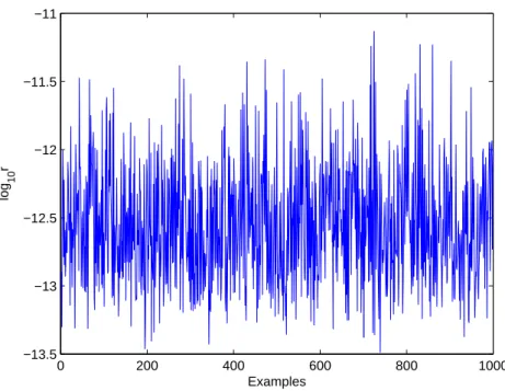
And then, we have carried out 1000 examples by using MATLAB , and the results of the computational simulation are illustrated in the Figure 4.1. Obviously, we see that log10r is located at the interval [−13.4867, −11.1319], that is, the relative
residual r can be regarded as nearly zero. In other words, given (X1, Λ1) ∈ R25×48×
R48×48, the QIEP has the nontrivial solution (M
g, Gg, Kg), even if the homogeneous
0 200 400 600 800 1000 −13.5 −13 −12.5 −12 −11.5 −11 Examples log 10 r
Figure 4.1: The computational simulation of log10r for 1000 examples.
5
Conclusions
It is often impossible to obtain the entire eigen-information for a large or complicated physical system. In general, it might be more sensible to consider the QIEP with only a portion of eigenvalues and eigenvectors. Therefore, we principally solve a general solution for the QIEP of gyroscopic system with partially prescribed matrix pair (Λ, X) ∈ Rm×m× Rn×m under assumptions A.1–A.3 in this paper. We derive
a complete theory on when a nonsingular quadratic pencil solution to the QIEP is possible.
At first, we describe a parameterized matrix representation for the general solution to the QIEP. An important characteristic in our construction for the general solution is that the parameters involve W and D described in Theorem 2.1 and in Lemma 2.1, respectively.
Secondly, we prove that the QIEP has a nonsingular quadratic pencil solution and has only singular quadratic pencil solutions when the number of the given
eigen-pairs, respectively, smaller and larger than a critical number k∗. Furthermore, the
dimension of the solution space for the QIEP have been characterized. These con-tributions made in Section 2 are significant.
Finally, we take advantage of some results to show an application of the QIEP for eigenvalue shifting. In addition, the results of numerical examples illustrate the efficiency of our method.
References
[1] P. Lancaster. Lambda-matrices and Vibrating Systems. Dover Publications, Dover edition, 1966.
[2] I. Gohberg, P. Lancaster, and L. Rodman. Spectral analysis of selfadjoint matrix
polynomials. Annals of Mathematics, 112:34–71, 1980.
[3] I. Gohberg, P. Lancaster, and L. Rodman. Matrix Polynomials. Academic Press, New York, 1982.
[4] B. N. Datta, S. Elhay, and Y. M. Ram. Orthogonality and partial pole
assign-ment for the symmetric definite quadratic pencil. Lin. Alg. Appl., 257:29–48,
1997.
[5] R.O. Hryniv, P. Lancaster, and A.A. Renshaw. A stability criterion for parameter-dependent gyroscopic systems. Journal of applied mechanics, 66:660–
664, 1999.
[6] P. Lancaster. Strongly stable gyroscopic systems. Electron. J. Linear Algebra, 5:53–66, 1999.
[7] F. Tisseur and K. Meerbergen. The quadratic eigenvalue problem. SIAM Rev., 43:235–286, 2001.
[8] J. Qian and W.W. Lin. A numerical method for quadratic eigenvalue problems
of gyroscopic systems. Journal of sound and vibration, 306:284–296, 2007. [9] M.T. Chu, W.W. Lin, and S.F. Xu. Updating quadratic models with no
[10] Y.F. Cai, Y.C. Kuo, W.W. Lin, and S.F. Xu. Solutions to a quadratic inverse