Using the Lagrange Relaxation Method to Solve the Routing and Packet Scheduling Problem in IEEE 802.16 Mesh Networks

(1)

1

Using the Lagrange Relaxation Method to Solve

the Routing and Packet Scheduling Problem in

IEEE 802.16 Mesh Networks

Meng-Hao Liu Pi-Rong Sheu Chi-Chiuan Liou Ren-Hao Liao Department of Department of Department of Department of Electrical Engineering Electrical Engineering Electrical Engineering Electrical Engineering National Yunlin University National Yunlin University National Yunlin University National Yunlin University of Science and Technology of Science and Technology of Science and Technology of Science and Technology Taiwan, ROC Taiwan, ROC Taiwan, ROC Taiwan, ROC

Email: g9612716@yuntech.edu.tw Email: sheupr@yuntech.edu.tw Email: liouchi@yuntech.edu.tw Email: g9812719@yuntech.edu.tw

Abstract―In an IEEE 802.16 mesh network, the routing and packet scheduling (RPS) problem is to design a fast scheduling scheme to meet the requirement of all the subscriber stations (SSs) so that all of the packets can be delivered to the base stations (BS) while minimizing the number of time slots and prohibiting the interference between any two packets. There has existed an integer linear programming formulation (ILPF) for the RPS problem, named as ILPF-for-RPS, which can find its optimal solution. However, the execution time of MIPF-for-MSC is very long when the number of SSs is large. This is because that the RPS problem has been proven to be NP-complete. In this paper, the Lagrange relaxation method is applied to shrink the solution space of the ILPF-for-RPS for the purpose of shortening the solution-searching time. First, we theoretically transform the ILPF-for-RPS into a Lagrange relaxation ILPF-for-RPS, whose objective function is then proved to be a concave function. This Lagrange relaxation ILPF-for-RPS simplifies the original ILPF-for-RPS and can be used to find an optimal solution for the RPS problem within a shorter time. According to the computer simulations, in contrast to the original ILPF-for-RPS, our Lagrange relaxation ILPF-for-RPS can attain a minimum time slot schedule within a shorter time for the RPS problem. To be more specific, compared with the original ILPF-for-RPS, our Lagrange relaxation ILPF-for-RPS can decrease the running time by more than 90% in most cases.

Index Terms―IEEE 802.16 mesh network, Lagrange relaxation, Linear programming, NP-complete, WiMAX technology.

I. INTRODUCTION

The IEEE 802.16 standard, also known as the WiMAX technology, is a technology of wireless network access which can service a large area. Its transmission rate exceeds 100 Mbps [1], which

qualifies itself to fit the category of high-speed wireless broadband network technology. Since the IEEE 802.16 standard adopts the multi-hop technique to deal with data packets among subscriber stations (SSs), only a few base stations (BSs) are required to cover a large metropolitan area. For this reason, an efficient routing and packet scheduling (RPS) algorithm is necessary to deal with SS-to-SS and SS-to-BS data transmissions. In fact, the RPS problem has recently become an important research topic in the multi-hop IEEE 802.16 standard [4][9][10][11][12] [15]. In this paper, we study the RPS problem in the IEEE 802.16 network and propose a fast method to solve it.

The multi-hop IEEE 802.16 standard can be subdivided into two types: mesh networks and mobile multi-hop relay networks. In this paper, mesh networks are concerned. In a mesh network, the objective of the RPS problem is to maximize the throughput of the network. In other words, the RPS problem is to design a fast scheduling scheme to meet the requirement of all the SSs so that all of the packets can be delivered to the BS while minimizing the number of time slots and

(2)

2

prohibiting the interference between any two packets.

Integer or mixed integer linear programming formulations [8] have been adopted by many researchers to solve various problems in wireless networks [2][3][5][14]. Similarly, there has existed an integer linear programming formulation (ILPF) for the RPS problem, named as ILPF-for-RPS, which can find its optimal solution [9]. However, the execution time of MIPF-for-MSC is very long when the number of SSs is large. This is because the authors of literature [9] have proven that the RPS problem is NP-complete for a general network topology. This means that it must take exponential time to find the optimal solution of the RPS problem.

As an approach to the ILPF of a NP-complete problem, an efficient computational methodology was proposed around 1970, namely, the Lagrange relaxation method [6][7]. The basic idea is that some constraints of a given ILPF can be relaxed so as to reduce the solution space, which in turn shortens the solution-searching time. In other words, this method relaxes the constraints which may otherwise make the running time of the ILPF of a combinatorial optimization problem become exponential. These relaxed constraints are merged into the objective function such that the original ILPF becomes a Lagrange relaxation ILPF. In general, an optimal solution to the resultant Lagrange relaxation ILPF can be obtained within a shorter period of time.

In this paper, the Lagrange relaxation method is applied to shrink the solution space of the ILPF-for-RPS for the purpose of shortening the solution-searching time. First, we theoretically

transform the ILPF-for-RPS into a Lagrange relaxation ILPF-for-RPS, whose objective function is then proved to be a concave function. This Lagrange relaxation ILPF-for-RPS simplifies the original ILPF-for-RPS and can be used to find an optimal solution for the RPS problem within a shorter time. In fact, to speed up the search of an optimal solution, we have cut down the solution space of the original ILPF-for-RPS. Our computer simulations show a decrease of the solution space by 37.73%. In other words, if the solution space must be searched by the original ILPF-for-RPS [9] in is 100%, our Lagrange relaxation ILPF-for-RPS can find an optimal time slot schedule with 62.27% of its solution space. Our method is feasible. This is because different schedules of minimum time slots usually exist in the RPS problem. We eliminate 37.73% of the solution space without completely eliminating all the minimum time slot schedules.

According to the computer simulations, in contrast to the original ILPF-for-RPS in [9], our Lagrange relaxation ILPF-for-RPS can attain a minimum time slot schedule within a shorter time for the RPS problem. To be more specific, compared with the original ILPF-for-RPS, our Lagrange relaxation ILPF-for-RPS can decrease the running time by more than 90% in most cases. In conclusion, our Lagrange relaxation method is demonstrated to be valuable for its contribution of a shorter solution time of the RPS problem.

The rest of this paper is organized as follows: In Section II, the RPS problem is described in detail and defined formally. In addition, an example is given to illustrate the RPS problem and its main constraints for packet transmissions. In Section III, the known ILPF-for-RPS is presented. In Section

(3)

3

IV, we apply the Lagrange relaxation method to the known ILPF-for-RPS, theoretically transform it into a Lagrange relaxation ILPF-for-RPS, and then prove the objective function of the Lagrange relaxation ILPF-for-RPS to be a concave function. In Section V, the performance of our Lagrange relaxation ILPF-for-RPS is evaluated and compared with that of the original ILPF-for-RPS through computer simulations. Finally, in Section VI, the conclusions of this study are drawn and our main contributions are stated.

II. PROBLEM DESCRIPTION

In this section, we present the RPS problem. In the RPS problem, a centralized scheduling is adopted. Therefore, the BS serves as the centralized schedulers for the entire network. In the following, the network considered is assumed to contain only one BS and several SSs. Each SS has packets to send to the BS. In this paper, we assume that the routing must follows the three constraints proposed by the literature [9].

(1) A SS cannot send and receive simultaneously. (2) There must be only one transmitter in the

neighborhood of a receiver.

(3) There must be only one receiver in the neighborhood of a transmitter.

A. Problem statement

Given a graph G=(V,E,w) and a transmission schedule S =(s₁,s₂,",s_m), where set V consists of a single BS: v₀ and multiple SSs:

1, , ,2 n

v v " v . E is the set of all links in G. If v _i

and v are within transmission ranges of each _j

other, then there exists a link (v_i,v_j)∈E . A packet-transmission function w :V → R+ is

defined. For each SS, it gives the number of packets that will be sent to BS. s_t ={V_t,E_t} is the transmission schedule at timeslot t , where V is _t

the transmitter set and E is the link set at timeslot _t t . The RPS problem is to find a routing tree and a

transmission schedule set S , so that only a minimal amount of timeslot is used to send all packets from each SS to BS.

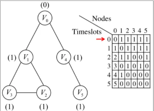
B. An example to illustrate the RPS problem Let us use the example in Figure 1 to illustrate the RPS problem. The network in Figure 1 consists of a BS: v and five SSs: ₀ v , ₁ v , ₂ v , ₃ v and ₄ v . ₅

In Figure 1, the number within braces adjacent to each node v shows the number of packets to be _i

sent from v to _i v . For example, the number ‘1’ ₀

in the braces next to v₁ means that there is one packet needs to be sent from v₁ to v for further ₀

process. For simplicity, in this example, we assume that each of the five SSs: v ,₁ v ,₂ v ,₃ v and ₄

5

v has only one single packet to be sent to BS.

That is, there are five packets in total to be sent to

0

v . Each column of the table in Figure 1

corresponds to each node: v , ₁ v , ₂ v , ₃ v and ₄ v . ₅

Each row represents a serial number denoting the timeslot. There are five timeslots in total which means all the packets from all the SSs can be sent to BS within five timeslots.

(1) (0) (1) (1) (1) (1) 0 V 2 V 1 V V₄ 3 V V₅ 0 0 0 0 0 5 0 0 0 0 1 4 0 1 0 1 0 3 1 0 0 1 1 2 1 1 1 1 0 1 1 1 1 1 1 0 5 4 3 2 1 0 5 4 3 2 1 0 Nodes Timeslots

(4)

4

In the beginning, the first row represents the state at timeslot 0 which no packets is received by

0

v and each SS has one packet to send. Next, at

timeslot 1, SS v₁ sent a packet to BS v . Hence, ₀

the value with v₁ is decreased to 0. At the same time, the value with v is increased by 1 to means ₀

that a packet is already received from v₁ . Meanwhile (at timeslot 1), all the nodes must obey the three routing constrains. As a result, v₁ can not receive packets from v₂ or v and send packets ₃

to v . Similarly, ₀ v can not receive packets ₀

from v₄ and receive packets from v₁. Therefore, there are still four packets waiting to be sent after

1

v sent a packet to v . At timeslot 2 ₀ v₁ served as a repeater while v sent a packet, i.e., ₃ v₁ retransmits the packet v . At the same time, ₀ v₄ also sends a packet to v . Therefore, there remain ₀

three packets to be sent in the entire network. At timeslot 3, v₁ sends the packet coming from v ₃

to v , and ₀ v sends its packet to ₅ v₄. Hence, there

are two packets waiting to be sent. At timeslot 4,

2

v then send its packet to v₁ while v₄ sends packet to v . Thus, only one packet is left to be ₀

transmitted. Finally, at timeslot 5, v₁ sends the packet to v . Thus, all the packets in the entire ₀

network have arrived at BS. Therefore, at least five timeslots are needed to send all the five packets from SSs to BS in Figure 1.

III. AKNOWN ILPF FOR THERPSPROBLEM In this section, we described a known ILPF for RPS problem: ILPF-for-RPS, provided by [9].

Variables used in ILPF-for-RPS are defined as follows: Y is a Boolean variable at timeslot t . _t

When all the packets have arrived at BS,Y_t =1;

Otherwise, 0Y_t = . R is a Boolean variable. _ij

When v is father of _j v , 1_i R_ij = ; Otherwise, 0

=

ij

R . X is a Boolean variable. When _ijt v _i

sends packets to v at timeslot t ,_j X_ijt =1 ; Otherwise, 0X_ijt = . w denotes the number of _it

packets to be sent in node v at timeslot t . _i A _t

denotes the number of packets that haven’t arrived at BS. U is an upper bound of timeslots in need. It is not hard to see that the number of required timeslots reaches the highest value when only one node sends a packet at each timeslot. That is, the highest value is equal to the sum of the products of packets in each node and the least hops from the node to the root.

Based on the above notation and definition, ILPF-for-RPS can be described as follows:

Objective function: Z_IP(RPS) =Minimize

∑

U_t₌₁tY_t (1) Subject to constrains: } , , 0 { }, , , 1 { n j n i E R_ij ≤ _ij ∀ ∈ " ∀ ∈ " (2) } , , 1 { 1 0R i n n j ij = ∀ ∈ "

∑

= (3) } , , 1 { }, , , 0 { }, , , 1 { n j n t U i R X_ijt _ij " " " ∀ ∈ ∀ ∈ ∈ ∀ ≤ ₍₄₎ 1 1 , {1, , }, {0, , }, {1, , } ikt jkt ijt jkt X X i j X X i j n k n t U + ≤ ∀ ≠ ⎧⎪ ⎨ ₊ _≤ ⎪⎩ ∀ ∈ " ∈ " ∈ " (5.1) (5.2) ( 1) {1, , } jt j t _i ijt _k jkt w w X X t U − = + − ∀ ∈

∑

" (6) } , , 1 { 1w t U A_t =

∑

_in₌ _it ∀ ∈ " (7)

(5)

5 1 1 =

∑

= U t Yt (8) } , , 1 { ) 1 ( 0 Y t U A A_t ≤ − _t ∀ ∈ " (9) ⎩ ⎨ ⎧ = = otherwise , 0 0 , 1 _t t A Y (10) ⎩ ⎨ ⎧ = otherwise , 0 of parent the is , 1 _j _i ij v v R (11)

1, sends a packet to at timeslot 0, otherwise i j ijt v v t X _{= ⎨}⎧ ⎩ (12)

Inequality (2) means that R_ij =1 only when link )(v_i,v_j exists. Equation (3) shows that each

i

v only has a single parent node. Inequality (4)

requires that v may send packets to _i v only _j

when link (v_i,v_j) exists in a multicast tree. According to the three routing constrains proposed by [9], Inequalities (5.1) and (5.2) are obtained. Equation (6) requires that the number of packets queued in v at timeslot t must be equal to the _i

number of the packets remained from the previous timeslots plus the number of packets received at the present timeslot, and minus the number of packets just sent. Equation (7) accumulates all the packets that have not arrived at BS in Variable A . _t

Equation (8) and Inequality (9) turn Y into 1 _t

when all the packets are received by BS at timeslot

t . The ranges of Y , _t R , and _ij X are specified _ijt

by functions (10) to (12), respectively.

The computational complexity of ILPF-for_RPS is _O(_n2_U) _{, where}_n _{is the} number of nodes and U is the unknown upper bound of total timeslots. Therefore, constrains (8)

and (9) of the ILPF-for-RPS will increase along with, such that the time for solving RPS problem will grow accordingly. In order to shorten the time for finding a solution, we will relax constrains (8) and (9).

IV. USING THE LAGRANGE RELAXATION

METHOD TO ANALYZE ILPF-FOR-RPS

A. Introduction to the Lagrange relaxation method

As an approach to the ILPF of a NP-complete problem, an efficient computational methodology was proposed around 1970, namely, the Lagrange relaxation method. The basic idea is that some constraints of a given ILPF can be relaxed so as to reduce the solution space, which in turn shortens the solution-searching time. In other words, this method relaxes the constraints which may otherwise make the running time of the ILPF of a combinatorial optimization problem become exponential. These relaxed constraints are merged into the objective function such that the original ILPF becomes a Lagrange relaxation ILPF. In general, an optimal solution to the resultant Lagrange relaxation ILPF can be obtained within a shorter period of time.

Let us use the following ILPF to illustrate the Lagrange relaxation method.

Objective function:

∑

= = n_t ₁c_ix_i IP Minimize Z _a (13) Constrains: j m j n i aijxi ≤b

∑ ∑

=1 =1 (14)

(6)

6 } , , 1 { and 0 x i n x_i≥ _i∈Ν ∀ ∈ " (15)

Constrain (15) denotes all variables

k

x x

x₁, ₂,", fall in the range of natural number N, and { |x i_i =1, 2... } 0k ≥ . In constrain (14), the sum of the products of each x and _i a is bounded by _ij

j

b . Now, suppose that the constrain (14) will make

the objective function be unable to minimize

∑

=

n

i 1cixi under polynomial time, we then relax

constrain (14) and merge it into the objective function to form a Lagrangian relaxation ILPF. Thus, the Lagrange relaxation ILPF can easily find the minimum of

∑

n₌

i 1cixi . The Lagrange

relaxation ILPF is composed of the objective function (13) and Constrains (14) and (15).

Relaxed objective function:

) ( Minimize ZLRa =

∑

=₁ + ⋅

∑ ∑

=₁ =₁ − m j n i ij i j n i cixi λ a x b (16) Relaxed constrain: } , , 1 { and 0 x i n x_i≥ _i∈Ν ∀ ∈ " , (17) where λ is Lagrange multiplier. We can modify λ so that the solution space can be reduced, which in turn speed up the solution-searching process.

B. Definitions and theorems

In this subsection, we propose several Theorems for RPS problem. First of all, we relax Equation (8) (i.e.

∑

U_t₌₁Y_t =1) and Inequality (9) (i.e.

t Y A

A_t ≤ ₀(1− _t) ∀ ) and merge them into

objective function (1)

(i.e. Z_IP(RPS) =Minimize

∑

U_t₌₁tY_t ) to transform MILP-for-RPS into a Lagrange relaxation MILP-for-RPS. This Lagrange relaxation MILP-for-RPS can shrink the solution space of original one and find an optimal solution in short time.

The Lagrange relaxation MILP-for-RPS is defined as follows:

Relaxed objective function:

{

(

)

[

]

}

∑

= = = − − ⋅ + − ⋅ + = U t t t U t t U t t Y A A Y tY λ 1 0 2 1 1 1 2 1 LR(RPS) ) 1 ( 1 Minimize ) , ( Z λ λ λ (18) where λ₁ and λ₂ are Lagrange multipliers.

Subject to Relaxed constrains:

Constrains (2), (3), (4), (5), (6), (7), (10), (11), and (12).

Definition 1: If there is a function Z x R

( )

: →R, and there exists three points x₁, x₂, and x₃ in [a,

b], such that a x< 1<x2 <x3<b and Z x

( )

2 ≥L x

( )

2 ,

where L x

( )

is a linear equation through Points

)) ( , (x₁ Z x₁ and (x₃,Z(x₃)) , then Z x

( )

is a concave function. Theorem 1: Let Q {Yk|k 1,2, ,K} t = " = be a

feasible solution set, where Q∈Ν. If Q is a

finite set, i.e., Q<∞, then

( )( )

(

)

1 1 0 1 , 1 1 U U k k t t t t U k k t t t t tY Y A A Y Y Q λ λ λ λ = = = ⎧ ⎛ ⎞ = _⎨ + ⋅_⎜ − _⎟ ⎝ ⎠ ⎩ ⎫ ⎡ ⎤ + ⋅ _⎣ − − _⎦ _{∈ ⎬} ⎭

∑

1 2 1 LR RPS 2 Z Minimize is a concave function.

(7)

7

Proof: Since Q {Yk|k 1,2, ,K}

t = "

= is a finite

feasible solution set, K

t t

t Y Y

Y1, 2,_", _{are feasible} solutions. Therefore, Function Z_LR(RPS)(λ₁,λ₂) can be expressed as follows: ( )( )

(

)

1 ₁ ₁ 0 1 , 1 1 U U k k t t k K _t _t U k t t t tY Y A A Y λ λ λ λ ≤ ≤ ₌ ₌ = ⎧ ⎛ ⎞ = _⎨ + ⋅_⎜ − _⎟ ⎝ ⎠ ⎩ ⎫ ⎡ ⎤ + ⋅ _⎣ − − _⎬ ⎦⎭

∑

1 2 1 LR RPS 2 Z Minimize

If )Z_LR(RPS)(λ₁,λ₂ has the minimum feasible

solution q t Y , then ( )( )

(

)

1 1 0 1 , 1 1 U U q q t t t t U q t t t tY Y A A Y λ λ λ λ = = = ⎛ ⎞ = + ⋅_⎜ − _⎟ ⎝ ⎠ ⎡ ⎤ + ⋅ _⎣ − − _⎦

∑

1 2 1 LR RPS 2 Z . Because

∑

U₌₁ −1=0 t Yt by (8), we can temporally

ignore λ₁ so that we rewrite Z_LR(RPS)(λ₁,λ₂) as

( )( ) 0

(

)

1 1 1 U U q q t t t t t tY A A Y λ λ = = ⎡ ⎤ =

∑

+ ⋅

∑

_⎣ − − _⎦ 2 2 LR RPS Z .

Now suppose that there exists a Lagrange

multiplier a b 2 2 * 2 α λ (1 α) λ λ = ⋅ + − ⋅ such that ) ( Z * 2

LR(RPS) λ has the largest solution space under

the minimum feasible solution q t Y , where ] 1 , 0 [ = α . We have ( )

( )

(

)

(

)

(

)

( )

(

)

0 1 1 0 1 ₁ ₁ 1 (1 ) (1 ) 1 (1 ) 1 (1 ) a b U U q a b q t t t t t a b U U k a k t t t k K _t _t t k K tY A A Y tY A A Y tY λ α λ α λ α λ α λ α λ α λ α λ α ∗ = = ≤ ≤ ₌ ₌ ≤ ≤ = ⋅ + − ⋅ ⎛ _⎡ _⎤⎞ = + ⋅ + − ⋅ ⋅_⎜ _⎣ − − _⎦_⎟ ⎝ ⎠ ≥ ⋅ + − ⋅ ⎛ ⎧ _⎡ _⎤⎫⎞ = ⋅_⎜ _⎨ + ⋅ _⎣ − − _⎦_⎬_⎟ ⎩ ⎭ ⎝ ⎠ + − ⋅

∑

2 2 2 LR RPS LR RPS 2 2 2 2 LR RPS LR RPS 2 Z Z Z Z Minimize Minimize 0

(

)

1 1 1 U U k b k t t t t A A Y λ = = ⎛ ⎧ ₊ _⋅ _⎡ ₋ ₋ _⎤⎫⎞ ⎨ ⎬ ⎜ _⎣ _⎦ ⎟ ⎩ ⎭ ⎝

∑

2

∑

⎠

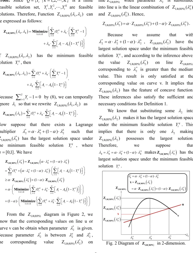
From the Z_LR(RPS) diagram in Figure 2, we know that the corresponding values on line u or curve v can be obtain when parameter *

2 λ is given. Because parameter * 2 λ is between a 2 λ and b 2 λ ,

the corresponding value Z ( *)

2

LR(RPS) λ on

line Z_LR(RPS) when parameter *

2

λ is substituted into line u is the linear combination of Z_LR(RPS)(_λ₂a)

and Z_LR(RPS)(_λ₂b)_{. Hence,}

*

LR(RPS) 2 LR(RPS) 2 LR(RPS) 2

Z ( )_λ _{= ⋅}_α Z ( ) (1_λa _{+ −}_α) Z_⋅ ( )_λb _.

Because we assume that with

b a 2 2 * 2 α λ (1 α) λ λ = ⋅ + − ⋅ , Z ( *) 2 LR(RPS) λ have the

largest solution space under the minimum feasible solution q

t

Y , and according to the inference above,

the value Z ( *)

2

LR(RPS) λ on line ZLR(RPS)

corresponding to * 2

λ is greater than the medium value. This result is only satisfied at the corresponding value on curve v. It implies that

) (

Z_LR(RPS) λ₂ has the feature of concave function.

These inferences also satisfy the sufficient and necessary conditions for Definition 1.

We know that substituting some λ₂ into )

(

Z_LR(RPS) λ₂ makes it has the largest solution space

under the minimum feasible solution q t

Y . This

implies that there is only one λ₂ making )

(

Z_LR(RPS) λ₂ possesses the largest solution.

Therefore, we suppose that

(1 )

a b

λ ₌λ∗ _{= ⋅}α λ _{+ −}α λ_⋅

2 2 2 2 makesZLR RPS( )

( )

λ2∗ has the

largest solution space under the minimum feasible solution q t Y . ( ) LR RPS Z (1 ) a b λ∗_{= ⋅}α λ _{+ −}α λ_⋅ 2 2 2 λ∗ 2 2 λ ( )

( )

λ2∗ LR RPS Z ( )

( )

λ2a LR RPS Z a λ2 b λ2 X ( )

( )

λ2b LR RPS Z ( )

( )

a (1 ) ( )

( )

b λ α λ α λ ∗ = = ⋅ + − ⋅ 2 LR RPS 2 2 LR RPS LR RPS x Z Z Z u v

(8)

8

It means that the solution space of ₍ ₎

( )

λ∗

2 LR RPS

Z

is greater than those of both ₍ ₎

( )

_λa

2 LR RPS Z and ( )

( )

λ2b LR RPS Z . That is to say, ( )

( )

λ2∗ > ( )

( )

λ2a LR RPS LR RPS Z Z and ( )

( )

λ2∗ > ( )

( )

λ2b LR RPS LR RPS Z Z . In this case, we rationalized ( )

( )

λ2∗ ≥ ⋅α ( )

( )

λ2a + −(1 α)⋅ ( )

( )

λ2b LR RPS LR RPS LR RPS Z Z Z , so it

can be claimed that ZLR RPS₍ ₎( )λ2 is a concave

function. Hence, we have showed that

( )( )λ2 ( )(λ λ1, 2) LR RPS LR RPS

Z = Z is a concave function.□

Theorem 2: If function Z_{LR RPS}₍ ₎( )λ₂ = Z_{LR RPS}₍ ₎(λ λ₁, ₂)

is a concave function, then there exists a parameter

λ∗ 2 and a set

{

| 1, 2, ,

}

i S= s i= " n such that ( )

( )

λ2∗ + ⋅si

(

λ λ2− 2∗

)

≥ ( )( )λ2 LR RPS LR RPS Z Z holds, where * 1 2 , , , ,_{s s} ,_sn _R λ λ ∀ " ∈ .

Proof: First of all, suppose that Z_{LR RPS}₍ ₎( )λ₂ is a

concave function. A set I=

{

( , ) |λ₂ Z Z≤Z_{LR RPS}₍ ₎( )λ₂

}

is given such that ( ,_λa _Za)

2 and ( ,λ2b Zb) both

belong to I . Thus, we can obtain a point

) , ( * *

2 Z

λ between ( ,_λa _Za)

2 and ( ,λ2b Zb) such that

) ) 1 ( , ) 1 ( ( ) , ( ) 1 ( ) , ( ) , ( 2 2 2 2 * * 2 b a b a b b a a Z Z Z Z Z ⋅ − + ⋅ ⋅ − + ⋅ = ⋅ − + ⋅ = α α λ α λ α λ α λ α λ

where α =

[ ]

0, 1 . By Theorem 1, we know that substituting _{α λ}_⋅ a_{+ −}(1 _{α λ})_⋅ b

2 2 into the concave

function Z_{LR RPS}₍ ₎( )⋅ can satisfy the following

condition: ( )

(

)

( )

(1 ) (1 ) (1 ) . a b a b a b Z Z α λ α λ α λ α λ α α ⋅ + − ⋅ ≥ ⋅ + − ⋅ = ⋅ + − ⋅ 2 2 LR RPS 2 2 LR RPS LR RPS Z Z Z

By Theorem 1, it can be found that the concave function ₍ ₎

(

_{α λ}_⋅ a_{+ −}(1 _{α λ})_⋅ b

)

2 2

LR RPS

Z will be

always greater than or equal to _α_⋅_Za_{+ −}(1 _α)_⋅_Zb_. Therefore, it is sure that the function passes through ( ,_λa _Za)

2 and ( , )

b _Zb

λ2 is not linear. In

this case, it can be guaranteed that the point

(

_{α λ}_⋅ a_{+ −}(1 _{α λ α})_⋅ b, _⋅_Za_{+ −}(1 _α)_⋅_Zb

)

2 2 between

( ,_λa _Za)

2 and ( ,λ2b Zb) belongs to set I. So, it can

be claimed that I is a convex set.

Suppose that there exists a point

( )

(

λ∗, λ∗

)

2 ZLR RPS 2 located at the margin of the

solution space of set I , and there exists an

orthogonal tangent plane ₍ ₎

( )

_λ∗ _{+ ⋅}_si

(

_{λ λ}₋ ∗

)

2 2 2 LR RPS

Z

which passes through

(

λ∗, ₍ ₎

( )

λ∗

)

2 ZLR RPS 2 and is

generated by _si _{. Let us let}_λ _<_λ∗

2 2 , then the

following can be satisfied:

( )

λ2∗ + ⋅si

(

λ λ2− 2∗

)

> LR( )λ2 LR RPS

Z Z

where _λ∗_{= ⋅}_{α λ}a_{+ −}(1 _{α λ})_⋅ b

2 2 2 and α =

[ ]

0, 1 .

With the above procedure,

( )

λ2∗ + ⋅si

(

λ2a−λ2∗

)

> LR

( )

λ2a LR RPS Z Z and ( )

( )

λ2∗ + ⋅si

(

λ2b−λ2∗

)

> LR

( )

λ2b LR RPS Z Z can be both

fulfilled. By further expanding these conditions, we can obtain the following inequality:

( )

{

}

( )

(1 ) (1 ) i a b a b s λ α λ α λ λ α λ α λ ∗ _{+ ⋅} _⎡ _⋅ _{+ −} _⋅ _⎤₋ ∗ ⎣ ⎦ ≥ ⋅ + − ⋅ 2 2 2 2 LR RPS 2 2 LR RPS LR RPS Z Z Z . Since parameter _si_⋅

{

_⎡_{α λ}_⋅ a_{+ −}(1 _{α λ})_⋅ b_⎤₋_λ∗

}

⎣ 2 2⎦ 2 is a very

small and negative value, it is even eliminated and

( )

λ2∗ ≥ ⋅α ( )

( )

λ2a + −(1 α)⋅ ( )

( )

λ2b LR RPS LR RPS LR RPS

Z Z Z still

holds. □ Definition 2: If Z_{LR RPS}₍ ₎: R→R is a concave

function, and there exist multiplier λ∗_∈R

2 and

parameter s R∈ such that

( )

( ) (

λ2∗ + ⋅s λ λ2− 2∗

)

≥ ( )( )λ2 LR RPS LR RPS

Z Z ∀ ∈λ₂ R , then

we denote s as a subgradient of Z_{LR RPS}₍ ₎( )⋅ at λ∗

2,

and the set consisting of subgradients generated by

( )( )⋅ LR RPS Z at λ∗ 2 is denoted as ( )

( )

λ λ ∗ ∗ ∂ ∂ LR RPS 2 2 Z .

(9)

9

relaxation formulation Z_{LR RPS}₍ ₎: R→R is a concave

function such that Z_{LR RPS}₍ ₎( )⋅ has the largest

feasible solution space (i.e.,

( )( )

max{Z_{LR RPS} λ₂ |λ₂∈R,λ₂ ≥0} ), after Lagrange

multiplier λ₂ converges to λ∗

2 and is substitute

into Z_{LR RPS}₍ ₎( )⋅ . Hence, λ2 converges to λ2∗ if

and only if ( )

( )

0 i s λ λ ∗ ∗ ∂ = = ∂ LR RPS 2 2 Z . Proof: By Definition 2, ( )

( )

λ2∗ + ⋅si

(

λ λ2− 2∗

)

≥ ( )( )λ2 LR RPS LR RPS Z Z holds and implies _si_⋅

(

_{λ λ}₋ ∗

)

_≥ ₍ ₎( )_λ ₋ ₍ ₎

( )

_λ∗ 2 2 ZLR RPS 2 ZLR RPS 2 .

Therefore, suppose that the necessary and sufficient condition of λ₂ converging to λ∗ 2 is a subgradient ( )

( )

0 i s _{= ∂ ∂}λ∗ λ∗ ₌ 2 LR RPS 2

/ Z , then it is clearly that

(

)

( )( ) ( )

( )

0_⋅ λ λ₋ ∗ _≥ λ ₋ λ∗ 2 2 ZLR RPS 2 ZLR RPS 2 holds, which leads ₍ ₎

( )

λ∗ _≥ ₍ ₎( )λ 2 2 LR RPS LR RPS Z Z . Because the

feasible solution space of ₍ ₎

( )

λ∗

2 LR RPS

Z is close to

the one of linear programming formulation Z_{IP RPS}₍ ₎ when Lagrange multiplier λ₂ converges to λ∗

2, the

feasible solution space of ₍ ₎

( )

λ∗

2 LR RPS

Z is larger

than that of Z_{LR RPS}₍ ₎( )⋅ at any other λ₂∈R, which

justifies our assumption. □

Theorem 4: If there exist several feasible solutions

1_, 2_, _, K

t t t

Y Y " Y for Z_{LR RPS}₍ ₎( )⋅ , in which a feasible solution k

t

Y makes the following be held:

( )

0

(

)

1 1 1 U U k k t t t k K _t tY _t A A Y λ∗ λ∗ ∈ ₌ ₌ ⎧ _⎡ _⎤⎫ = _⎨ + ⋅ _⎣ − − _⎦_⎬ ⎩

∑

⎭ 2 2 LR RPS Z Minimize

Therefore, given a set

( )

0

(

)

1 1 1 U U i i t t t t t M i λ∗ tY λ∗ A A Y = = ⎧ _⎡ _⎤⎫ =_⎨ = + ⋅ _⎣ − − _⎦_⎬ ⎩ ZLR RPS 2

∑

2

∑

⎭,

then there exists a subgradient for any i M∈

( )

0

(

)

1 1 U i i t t t s λ A A Y λ∗ ∗ = ∂ _⎡ _⎤ = = _⎣ − − _⎦ ∂ LR RPS 2

∑

2 Z where _si_{is a subgradient of} ( )( )⋅ LR RPS Z at λ∗ 2 , and _si _{⊆ ∂ ∂}/ _λ∗ ₍ ₎

( )

_λ∗

2ZLR RPS 2 . If each element i in set

M satisfies the following equation

( )

0

(

)

1 1 U i i t t t s λ A A Y λ ∗ ∗ = ∂ _⎡ _⎤ = = _⎣ − − _⎦ ∂ LR RPS 2

∑

2 Z , then at λ∗

2, ZLR RPS( )( )⋅ has multiple subgradients: ( )

( )

, 1, 2, , i s λ i n λ ∗ ∗ ∂ ⊆ = ∂ LR RPS 2 2 Z " . Proof:

(

)

(

) (

)

(

)

(

)

( )( ) ( )

( )

(

)

( )( ) 0 1 0 0 1 1 1 1 1 i U i t t t U U i i t t t t t t i s A A Y A A Y A A Y s λ λ λ λ λ λ λ λ λ λ λ λ ∗ ∗ = ∗ = = ∗ ∗ ∗ ⋅ − ⎡ ⎤ = _⎣ − − _⎦⋅ − ⎧ _⎡ _⎤⎫ ⎧ _⎡ _⎤⎫ = ⋅⎨ _⎣ − − _⎦⎬− ⋅⎨ _⎣ − − _⎦⎬ ⎩ ⎭ ⎩ ⎭ ≥ − ⇒ + ⋅ − ≥

∑

2 2 2 2 2 2 2 2 LR RPS LR RPS 2 2 2 2 LR RPS LR RPS Z Z Z Z

By Definition 2, we know that _si_{is a subgradient}

( _si _{is defined by} ( )

( )

0

(

)

∑

2 Z ).

With a similar inference, it can be justified that each element i=1, 2,",n in set M satisfies the

equation ( )

( )

0

(

)

∑

2 Z . Hence at λ∗

2, ZLR RPS( )( )⋅ has multiple subgradients:

_si ₍ ₎

( )

_λ ,_i 1, 2, ,_n λ ∗ ∗ ∂ ⊆ = ∂ LR RPS 2 2 Z " □

C. The choice of Lagrangian parameter λ₂ By Theorem 1 and Theorem 2, Z_{LR RPS}₍ ₎( )λ₂

has been proved to be a concave function. Therefore, there must exist exactly one λ∗

2 in our

(10)

10

space of ₍ ₎

( )

λ∗

2 LR RPS

Z contains the optimal feasible

solution Y_t∗. According to Theorem 4, we first substitute λ∗

2 into ZLR(RPS)(), and then we choose

a subgradient _s*_{from the generated subgradient}

set _{∂ ∂}/ λ∗ ₍ ₎

( )

λ∗ 2ZLR RPS 2 . If * s complies with Theorem 3 (i.e., _si _{= ∂ ∂}/ _λ∗ ₍ ₎

( )

_λ∗ ₌0 2ZLR RPS 2 ), then λ2

has converged to the optimal λ∗

2 . Finally,

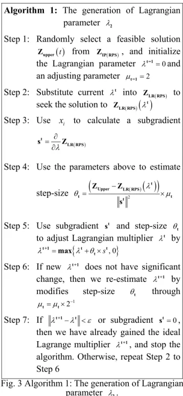
according to those theorems above, we establish Algorithm 1 (see Figure 3) to generate Lagrangian parameter λ₂.

V. COMPUTER SIMULATIONS

In the computer simulation, our hardware contains a PC with two Intel(R) Pentium(R) IV CPU runs at 3.40GHz and 1014MB RAM. In software aspect, we use C/C++ and LINGO 8.0 [13].

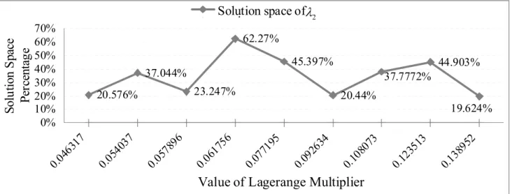
Figure 4 shows our computer simulation results. When the Lagrange parameter λ₂ comes to 0.061756, the resultant solution space is 62.27% of the one searched by the original ILPF-for-RPS. In other words, we reduce 37.73% computation for scheduling, which in turn saves about 1/3 computational time.

The performance benchmarks reflect CPU execution time. In Table 1, with 9 nodes, the original ILPF-for-RPS Z_IP(RPS) needs 7 minutes and 50 seconds to solve the RPS problem while our Lagrange relaxation ILPF-for-RPS Z_LR(RPS) only spends 10 seconds to find the optimal solution. In Table 1, there is no case with more than 17 nodes because the execution time of Z_IP(RPS) exceeds 3600 minutes. The execution time is too long, so we stop to increase the number of nodes in our simulations. Compared with the original ILPF-for-RPS, Table 1 shows that with different

numbers of nodes: 9, 11, 13, and 15, our Lagrange relaxation ILPF-for-RPS can decrease running time by 97.87%, 90.24%, 69.91%, and 96.50%, respectively. While a network containing 17 nodes, the CPU execution time can be reduced from more than 3600 minutes to 31 minutes and 36 seconds.

Algorithm 1: The generation of Lagrangian parameter λ₂

Step 1: Randomly select a feasible solution

( )t

upper

Z from ZIP RPS₍ ₎ , and initialize

the Lagrangian parameter λt =1=0_and

an adjusting parameter μ =_t=1 2

Step 2: Substitute current λt_into

( )

LR RPS

Z to

seek the solution to ₍ ₎

( )

λt LR RPS

Z

Step 3: Use x to calculate a subgradient _i

( ) λ ∂ = ∂ t LR RPS s Z

Step 4: Use the parameters above to estimate

step-size θ =

(

− ₂( )

( )

λ

)

×μ t Upper LR RPS t _t t Z Z s

Step 5: Use subgradient _st_{and step-size}_θ t

to adjust Lagrangian multiplier λt _by

{

s, 0

}

λt +1 = λ θt+ × t t

max

Step 6: If new λt +1_{does not have significant}

change, then we re-estimate λt +1 _by

modifies step-size θ_t through

1

2 μ ₌μ _× −

t t

Step 7: If λt +1−λt <ε_{or subgradient}_st ₌₀_,

then we have already gained the ideal Lagrange multiplier λt +1_{, and stop the}

algorithm. Otherwise, repeat Step 2 to Step 6

Fig. 3 Algorithm 1: The generation of Lagrangian parameter λ₂.

(11)

11 19.624% 44.903% 37.7772% 20.44% 45.397% 62.27% 23.247% 37.044% 20.576% 0% 10% 20% 30% 40% 50% 60% 70% 0.04 6317 0.054 037 0.05 7896 0.061 756 0.07 7195 0.09 2634 0.10 8073 0.12 3513 0.1389 52

Value of Lagerange Multiplier

So lu tio n S pa ce Pe rc en ta ge Solution space of i

Fig. 4 Quality of Lagrange Multiplierλ₂.

Table 1 The execution time of ILPF-for-RPS and Lagrange relaxation ILPF-for-RPS with Lagrange Multiplier λ₂ =0.061756

Function ZIP(RPS) ZLR(RPS) ZIP(RPS) ZLR(RPS) ZIP(RPS) ZLR(RPS) ZIP(RPS) ZLR(RPS) ZIP(RPS) ZLR(RPS) Number

of Nodes 9 11 13 15 17

Timeslots 12/16 12/16 14/21 14/21 25/32 25/32 24/25 24/25 xx/44 27/44

Execution Time(m:s) 07:50 00:10 28:52 02:49 52:31 15:48 316:04 11:04 Over_{3600:00 31:36}

Feasible Solution

Probability 100% 100% 100% 100% 100% 100% 100% 100% xx% xx%

These simulation results imply that our Lagrange relaxation ILPF-for-RPS can reduce the solution-finding time significantly.

VI. CONCLUSIONS

In this paper, we have studied the RPS problem in a mesh network. The RPS problem has been proven to be NP-complete and an ILPF for its optimal solutions has been proposed. However, the existing ILPF-for-RPS has a heavy execution time. This makes the finding of the optimal solutions of the RPS problem impractical in most situations. In this paper, the Lagrange relaxation method has

been applied to shrink the solution space of the ILPF-for-RPS for the purpose of shortening the solution-searching time. We have transformed the ILPF-for-RPS into a Lagrange relaxation ILPF-for-RPS. Further, we have proved the objective function of our Lagrange relaxation ILPF-for-RPS to be concave. Computer simulation results show that, in contrast to the original ILPF-for-RPS, our Lagrange relaxation ILPF-for-RPS can decrease the running time by more than 90% in most cases. To sum up, our Lagrange relaxation ILPF-for-RPS simplifies the original ILPF-for-RPS and can be used to find an

2 λ

(12)

12

optimal solution for the RPS problem within a shorter time.

ACKNOWLEDGEMENTS

This work was supported in part by the National Science Council of the Republic of China under Grant No. NSC 96-2221-E-224-005-MY2.

REFERENCES

[1] Z. Abichar, Y. Peng, and J. M. Chang, “WiMAX: The emergence of wireless broadbnad”, IT Professional, Vol. 8, Issue 4, pp.44-48, July-August 2006.

[2] A. K. Das, R. J. Marks, M. El-Sharkawi, P. Arabshahi, and A. Gray, “Minimum power broadcast trees for wireless networks: integer programming formulations,” Proceedings of the Twenty-Second Annual Joint Conference of the IEEE Computer and Communications Societies (IEEE INFOCOM 2003), Vol. 2, pp.1001-1010, 2003.

[3] A. K. Das, R. J. Marks, M. A. El-Sharkawi, P. Arabshahi, and A. Gray, “Optimization methods for minimum power multicasting in wireless networks with sectored antennas,” Proc. of IEEE Wireless Communications and Networking Conference, pp.1299-1304, March 2004.

[4] D. Ghosh, A. Gupta, and P. Mohapatra, “Scheduling in multihop WiMAX Networks,” ACM SIGMOBILE Mobile Computing and Communications Review, Vol. 12, Issue 2, pp.1-11, April 2008.

[5] S. Guo and O. W. Yang, “Minimum-energy multicast routing in static wireless ad hoc networks,” Proc. of IEEE International Conference on Network Protocols (ICNP'04), Vol. 6, pp.3989-3993, September 2004.

[6] M. Held and R. M. Karp, “The traveling salesman problem and minimum spanning trees,” Institute of Operations Research (INFORMS 1970), Vol. 18, pp.1138-1162, 1970.

[7] M. Held and R. M. Karp, “The traveling salesman problem and minimum spanning trees: part II,” Proceedings of the 7th Mathematical Programming Symposium, Vol. 1, No. 1, pp.6-25,

December 1971.

[8] F. S. Hillier and G. J. Lieberman, “Introduction to Mathematical Programming,” 2nd ed., McGraw-Hill, 1995.

[9] F. Jin, A. Arora, J. Hwang, and H.-A. Choi, “Routing and packet scheduling for throughput maximization in IEEE 802.16 mesh networks,” Proceedings of IEEE Broadnets, September 2007. [10] H. Shetiya and V. Sharma, “Algorithms for routing

and centralized scheduling to provide QoS in IEEE 802.16 mesh networks,” Proceedings of the 1th ACM Workshop on Wireless Multimedia Networking and Performance Modeling (WMuNeP’05), New York, NY, USA, pp.140-149, October 2005.

[11] H. Shetiya and V. Sharma, “Algorithms for routing and centralized scheduling in IEEE 802.16 mesh networks,” Proceedings of Wireless Communications and Networking Conference (WCNC 2006), pp.147-152, April 2006.

[12] J J. Tao, F. Liu, Z. Zeng, and Z. Lin, “Throughput enhancement WiMAX mesh networks using concurrent transmission,” Proceedings of 2005 International Conference on Wireless Communications, Networking and Mobile Computing, Vol. 2, pp.871-874, September 2005. [13] K. Thornburg and A. Hummel, “LINGO 8.0

Tutorial: Introduction to LINGO 8.0,” http://www.icaen.uiowa.edu/~ie166/Private/Lingo. pdf

[14] C. Wang, M. T. Thai, Y. Li, F. Wang, and W. Wu, “Minimum coverage breach and maximum network lifetime in wireless sensor networks,” Global Telecommunications Conference (IEEE GLOBECOM 2007), pp.1118-1123, November 2007.

[15] H.-Y. Wei, S. Ganguly, R. Izmailov, and Z. J. Haas, “Interference-aware IEEE 802.16 WiMAX mesh networks,” Proceedings of 61st IEEE Vehicular Technology Conference (VTC 2005 Spring), Vol. 5, pp.3102-3106, 29 May-1 June 2005.