Robust Beamforming Based on the Least-Squared Method of Subarrays for Imperfect Antenna Array

全文

(1)Int. Computer Symposium, Dec. 15-17, 2004, Taipei, Taiwan.. Robust Beamforming Based on the Least-Squared Method of Subarrays for Imperfect Antenna Array Rungsak Niemkhum* and Raungrong Suleesathira** Department of Electronic and Telecommunication Engineering King Mongkut’s University of Technology Thonburi, Tungkru, Bangkok, Thailand 10140 Phone: +66-2-470-9074, Fax: +66-2-4709070, *E-mail: [email protected] , ** E-mail: [email protected]. Abstract-This paper presents an approach to array beamforming in the presence of array imperfections. The least-squared method of subarrays is used to improve the performance of the optimal beamformer. The proposed beamformer has a constraint that ensures that the desired signal passes through the processor undistorted in the look direction. It is also capable of nulling in the directions of co-channel interference. The simulations are done in the scenarios of white noise and colored noise. A significant performance improvement over the optimal beamformer is achieved in features of low sidelobes, undistorted desired signal, high output SINR and high array gain. Furthermore, the results demonstrate that the least-squared technique of subarrays is robust to array gain perturbation and to strong co-channel interference as compared to the ideal beamformer. Keywords: array imperfections, least-squared, subarrays, white noise, colored noise. 1.Introduction Recently, the increased demand for mobile communication systems has motivated the need for more efficient use of the RF spectrum. As a result, many efforts have been made for the beamforming algorithm promising to smart antennas. Beamformer exploits the spatial dimension to suppress interferences and prevent signal cancellation. Several beamforming algorithms are designed under the assumption of ideal signal characterizations and perfect antenna arrays. Approaches to robust beamforming in the presence of steering vector error are presented in [1-2]. The penalty function is added to the optimal weight to remedy beam distortion due to steering vector error [1]. The penalty function requires much computation. Iteratively searches for the correct steering vector by maximizing the array mean output power using a first-order Taylor series can combat against beam-steer error [2]. One development of robust array processor over the minimum variance beamforming is done by minimizing output power plus a penalty function, proportional to the square of the norm of the weight vector [3]. In the presence of an arbitrary unknown signal steering vector mismatch, minimization of a quadratic function subject to infinite many noncovex quadratic constraints is a new approach to robust adaptive beamforming [4]. For imperfect antenna array, a datadomain signal subspace updating algorithm is expressed. from the cause of cancelling the desired signal using the array covariance matrix of the perturbed model [5]. The H α algorithm is used to improve the performance of imperfect antenna array with the generalized sidelobe canceller structure [6]. In this paper, the application of the least-squared technique to the imperfect array beamforming is investigated to reduce sidelodes, maintain mainbeam in the look direction and suppress co-channel interferences. The initial antenna array is divided into subarrays. The weights of a subarray are provided by using the optimal weight. Then, the least-squared minimization between a beampattern reference and weight beampatterns of subarrays provides a better beampattern with low sidelobes, unity response in the direction of arrival of desired signal and null response in the direction of arrival of interference. The rest of this paper is organized as follows: Section 2 explains the signal models in the perfect and imperfect antenna arrays. Optimal beamformer is described in the section 3. A robust beamformer based on the least-squared minimization of subarrays is presented in section 4. Simulation results provided in section 5 demonstrate the performance of the proposed method compared to the optimal beamformer and ideal beamformer in the presence of array imperfections. Besides the modeling disturbance, white Gaussian noise and color noise are accounted in dealing with imperfect array beamforming. Finally, our conclusion are given in section 6.. 2. Array Signal Models th. The received array data at the n snapshot from M narrowband sources impinging on a uniform linear array with L antenna elements in the far field pattern can be represented as an L × 1 vector form [8] x(n) = As(n) + η(n) n = 0,..., N − 1 (1) where A = [a(θ1 ),K , a(θ M )] L×M is a steering matrix of a signal source s( n) = [ s1 ( n)K s M ( n)]M ×1 arriving T. [θ1 ,...,θ M ] and corrupted by a vector T noise η( n) = [n1 ( n),..., n L ( n)]L×1 which is spatially and. from direction θ =. temporally Gaussian noise with power vector of the m. 292. th. source is given by. σ n2 . The steering.

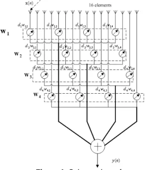
(2) Int. Computer Symposium, Dec. 15-17, 2004, Taipei, Taiwan.. a(θ m ) = [1 e. − j 2π. d. λ. sin θ m. ,..., e. d − j 2π ( L −1) sin θ m. λ. T L×1. ]. which. depends on an inter-element distance d , wavelength of the carrier λ and the impinging angle with respect to the array broadside θ m . Note that the superscript T denotes the transposition operator and N is the number of snapshots. Unlike the above perfect array, amplitude and phase of array element can be perturbed due to imperfect array structure. In the presence array imperfections, the signal model with gain perturbations G is written as [5-6] x(n) = GAs(n) + η(n) (2) ∆. [. where G = diag g1 ,..., g L. ]L×L. represents the complex. antenna gain matrix and gain g l can be modeled as. 4. Robust Beamforming against Imperfect Antenna Array The proposed beamformer is obtained by solving the least-squared problem given by [7] K. min ∑ P (θ ) − ∑ d k S k (θ ) dk. θ. complex gain perturbation of the l variance given by ∆. [. σ g2 = E ∆g l. 2. ]. th. ∑d. subject to. k =1. where. θd. 2. k =1. K. th. where ∆g l = ∆al + j∆pl represents a zero mean. (8). is used. However, the optimal beamformer is basically designed for the perfect array with the modeling disturbances, its degraded performance results in high sidelobes and distorted mainbeams. In the next section, we present an approach to achieve both sidelobe reduction and unity response of the mainbeam in the look directions.. g l = (1 + ∆al )e j∆pl l = 1,..., L (3) where ∆al and ∆p l are zero-mean random amplitude and phase errors of the l antenna element, respectively. Assuming that amplitude and phase errors are small yields an approximation of gl as g l ≈ 1 + ∆g l (4). 1 N −1 x ( n) x H ( n ) ∑ N k =0. R=. S k (θ d ) = 1. k. (9). is the directions of arrival of desired signals.. P (θ ) is reference array pattern ( taken here using the optimal weight ) expressed as L. element and have the. P (θ ) = ∑ w e * l. l =1. l = 1,..., L. − j 2π. d. λ. (l −1)sin θ. .. (10). th. where E denotes the expectation operator.. The array pattern of the k subarray with Q antenna elements can be computed by. 3. Optimal Beamformer. S k (θ ) = ∑ wq* (k )e. (5). Q. w = [w1 ,..., wL ]L×1 as [3-4] T. y (n) = w H x(n ) (6) where the superscript H stands for conjugate transposition. The weight vector of the optimal beamformer is obtained by. min w Rw Subject to A w = f H. H. w. It is equivalent to minimizing the array output but still maintaining the desired signal power. The vector f is an M × 1 vector specifying the desired response in the look directions and null response in the interference directions.. [. For instance, f = 1. θ1. 0...0]. and nulls in the directions at. 2π. λ. [( k −1)+Q( q−1)]d sinθ. k = 1,..., K. (11). q =1. The output of a beamformer can be formed by a sum of the array signals multiplied by a complex weight. T M ×1. −j. where w( k ) = [ w1 ( k ),..., wQ ( k )]Q×1 is the weight vector T. th. of the k subarray computed by Eq. (7). and K is the number of subarrays The d k ’s are the weights obtained by Eq. (9). which can be rewritten as. min P − Sd. The least-squared weights are then given by. (. −1. f .. Q. S f (θ ) = ∑Wq e. H. −j. 2πd. λ. Q ( q −1) sin θ. (13). q =1. where Wq =. (7). The covariance matrix R = E[ x( n) x ( n)] is unavailable in practical applications. Instead, the sample covariance matrix. −1. The array pattern based on least-squared minimization is then taken as. solution for the optimal weight vector can be found as. ). ). d = S H S [S H P − λb] (12) T H −1 −1 T H −1 H where λ = [b (S S) b] [b (S S) (S P) − 1] .. θ i i = 2,..., M . The. (. T. d. provides unity response at. w opt = R −1 A A H R −1 A. subject to d b = 1. 2. −j. K. ∑d k =1. k. w(k ) e * q. 2πd. λ. ( k −1) sin θ. .. To evaluate the performance of the proposed beamformer, we compare with the output SINR and array pattern of the optimal beamformer obtained in the previous section and. 293.

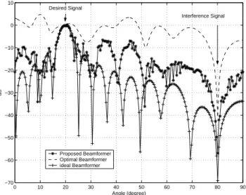
(3) Int. Computer Symposium, Dec. 15-17, 2004, Taipei, Taiwan.. that of the ideal beamformer. Having known gain perturbation matrix, the ideal weight vector can be found as [5]. w=. Ga(θ d ) . a (θ d )Ga(θ d ) H. (14) The output SINR can be calculated as. SINRout =. wH Rsw wH RNw. (15). where R s is a covariance matrix of desired signal . R N is a covariance matrix of interference plus noise which can be H. estimated as E[ x( n) I x I ( n)] and let. x I (n) = GAs I (n) + η(n) be the array signal of the interference source s I ( n) disturbed by noise, η(n) .. H ( z ) = 9(1 − 0.95 z −1 ) −1 is designed to filter a white. 5. Simulation Results To illustrate the performance of the proposed techniques and compare it with the optimal and ideal beamformers, simulation examples are presented under additive white Gaussian and colored noise environments. In all simulation, a 16-element linear array with half wavelength separation was divided into four subarrays as depicted in Fig 1. Also, the desired signal and interference signal have the same frequency arriving from different directions at 20° and 80°, respectively. The interference signal is stronger than the desired signal with the input SNR = 20dB, the input INR= 60 dB and the input SINR = 40 dB compared to background white noise of variance of gain error is fixed at. σ g2. σ n2. = 1. The. = 0.01. The number. of snapshots is 100. The results obtained are averaged 100 independent trials. In the first example, an imperfect array in the presence of white Gaussian noise is simulated to demonstrate the robustness of least-squared beamformer. Fig. 2(a) shows the array patterns using the optimal weight, our proposed weight and the ideal weight. It is obvious that the leastsquared method can maintain the mainbeam in the look direction and the null in the interference direction besides reducing the sidelobes. Notice that the optimal beamformer has very high sidelobe power. The output SINRs are calculated at different the number of snapshots for perfect and imperfect arrays as plotted in Fig. 2(b). For the perfect array, the least-squared based beamformer converges to the maximum output SINR faster than the optimal beamformer. In the presence of gain perturbation, the output SINR computed by using the least-squared technique is greater than that of using the optimal beamformer. From Fig. 2(c). consider the output SINR’s using the optimal beamformer. The resulting output SINR’s higher than the fixed input SINR’s at 0 dB and -40 dB regardless of gain error. σ g2. the interval (-70)-(-20) dB. Augmented with the leastsquared technique, array gain (SINRout/SINRint) can be however achieved much higher as seen in the plots of Fig. 2(c). Low sidelobes, unity mainbeam in the look direction, deep null in the non-look direction and high output SINR are qualified for our proposed beamformer on least-squared subarrays. Fig. 3 shows a beampattern obtained by using a 20-element linear array with half wavelength separation, divided into five subarrays. Clearly, the least-squared method can maintain the mainbeam in the look direction and suppresses the interference signal in the undesired direction besides reducing the sidelobes and close to that resulting from the ideal beamformer. A 24-element array with a space of half wavelength was divided into eight subarrays. The resulting array patterns in Fig. 4. corresponds to that of Fig. 3. We deal with imperfect array beamforming in a color noise scenario as the second example. The transfer function Gaussian noise for generating the colored noise. The beampattern comparison in Fig. 5(a) reveals that the leastsquared based beamformer performs as well as the ideal beamformer knowing the exact gain perturbation matrix. Fig. 5(b) illustrates that we have the output SINR decreases versus the number of snapshots in the case of imperfect array. However, the resulting output SINR is larger than the input SINR (-40dB). Compared to the optimal beamformer, the output SINR from the proposed beamformer has higher array gain in the both cases of perfect and imperfect arrays. Similarly to Fig. 2(c), the output SINR’s versus variance gain of error in Fig. 5(c) at each fixed input SINR. indicate that array gains can be achieved using the least-squared algorithm.. 6. Conclusions A robust beamforming method based on the leastsquared minimization of subarrays for imperfect antenna array is presented. Subarrays provide us a variety of beampatterns. The robustness is obtained by minimizing the difference between the beampattern reference and a sum of weighted subarray beampatterns. Compared to the optimal and ideal beamformers, the simulation results reveal that the proposed beamformer provides a satisfactory performance with the properties of low sidelobes, undistorted desired signal, co-channel interference suppression and high output SINRs.. for. 294.

(4) Int. Computer Symposium, Dec. 15-17, 2004, Taipei, Taiwan.. 10. References. Desired Signal Interference Signal. 0. [1] L. Rongfeng, W. Yongliang and W. Shanhu, “Robust Adaptive Beamforming Based on Penalty Function Under Steering Vector Errors,” 6th International Conference on Signal Processing 2002, Vol. 1, pp.321-324, Aug. 2002. [2] M. H. Er and B. C. Ng, “A New Approach to Robust Beamforming in the Presence of Steering Vector Errors,” IEEE Transactions On Signal Processing, Vol. 42, pp. 1826 - 1829, July 1994. [3] R. G. Lorenz and S. P. Boyd, “Robust Minimum Variance Beamforming,” 2003 The Thrity-Seventh Asilomar Conference on signals, Systems and Computers, Vol. 2, pp. 1345 - 1352, Nov. 2003. [4] S. A. Vorobyov, A. B. Gershman and Z. Q. Luo , “Robust Adaptive Beamforming Using Worst-Case Performance Optimization: A Solution to the Signal Mismatch Problem,” IEEE Transactions on Signal Processing, Vol. 51, No. 2, pp. 313 - 324, Feb. 2003. [5] W. S. Youn and C. K. Un, “Robust Adaptive Beamforming Based on the Eigenstructure Method,” IEEE Transactions on Signal Processing, Vol. 42, No. 6, pp. 1543- 1547, June 1994. [6] A. C. Chang and C. T. Chiang, “Adaptive H∞ Robust Beamforming for Imperfect Antenna array,” Signal Processing, Vol. 82, No. 8, pp. 1183-1188, Aug. 2002. [7] F. Cakrak and P. J. Loughlin, “Instantaneous Frequency Estimation of Polynomial Phase Signals,”. Proceedings of the IEEE-SP International Symposium on Time-Frequency and Time-Scale Analysis, pp. 549 – 552, Oct. 1998. [8] R. Suleesathira, “Close Directions of Arrival Estimation for Multiple Narrowband Sources, ” 7th International Symposium on Signal Processing and Its Applications, pp.403-406, Jul. 2003. −10. dB. −20. −30. −40. −50. −60. −70. Optimal beamformer Proposed Beamformer ideal Beamformer 0. 10. 20. 30. 40 50 Angle (degree). 60. 70. 80. 90. (a) 40. 30. 20. Output SINR(dB). 10. 0 Proposed Beamformer(Imperfect) Optimal Beamformer(Imperfect) Proposed Beamformer Optimal Beamformer. −10. −20. −30. −40. −50. 0. 100. 200. 300. 400 500 600 Number of Snapshots. 700. 800. 900. 1000. (b) 45 Proposed Beamformer Optimal Beamformer 40. 35. SINR = 0 dB int. Output SINR(dB). 30 SINR = − 40 dB int. 25 SINR = 0 dB int. 20. 15. 10. SINR = − 40 dB int. 5. 0. −5 −70. −65. −60. −55. −50 −45 −40 Variance of Gain Error(dB). −35. −30. −25. −20. (c). Figure 1. Subarray beamformer. Figure 2. Using 16 elements for 4 subarrays with additive white Gaussian noise (a) Beampatterns (b) Output SINR versus N for perfect and imperfect arrays and (c) Output SINR versus = 0 dB and -40 dB. 295. σ g2. for input SINR.

(5) Int. Computer Symposium, Dec. 15-17, 2004, Taipei, Taiwan. 10. 10. Desired Signal. Desired Signal. Interference Signal 0. 0. Interference Signal. −10 −10 −20 −20. dB. dB. −30 −30. −40 −40 −50 −50 −60 Proposed Beamformer Optimal Beamformer ideal Beamformer. −70. −80. 0. 10. 20. 30. Optimal beamformer Proposed Beamformer ideal Beamformer. −60. 40 50 Angle (degree). 60. 70. 80. −70. 90. 0. 10. 20. 30. 40 50 Angle (degree). 60. 70. 80. 90. (a) Figure 3. Beampatterns using 20-element array divided into 5 subarrays. 40. 30. 20. 10. 10 Output SINR(dB). Desired Signal Interference Signal 0. −10. 0 Proposed Beamformer(Imperfect) Optimal Beamformer(Imperfect) Proposed Beamformer Optimal Beamformer. −10. −20. −20. dB. −30. −30 −40. −40. −50. 0. 100. 200. 300. 400 500 600 Number of Snapshots. −50. 800. 900. 1000. (b) 60. Proposed Beamformer Optimal Beamformer ideal Beamformer. −60. −70. 700. Proposed Beamformer Optimal Beamformer 50. 0. 10. 20. 30. 40 50 Angle (degree). 60. 70. 80. 90 SINR = 0 dB int. Output SINR(dB). 40. Figure 4. Beampatterns using 24-element array divided into 8 subarrays. SINR = − 40 dB int 30 SINR = 0 dB int SINR = − 40 dB int. 20. 10. 0 −70. −65. −60. −55. −50 −45 −40 Variance of Gain Error(dB). −35. −30. −25. −20. (c) Figure 5. Using 16 elements for 4 subarrays with additive colored noise (a) Beampatterns (b) Output SINR versus N for perfect and imperfect arrays and (c) Output SINR versus -40 dB. 296. σ g2. for input SINR = 0 dB and.

(6)