Mining Frequent Itemsets for data streams over Weighted Sliding
Windows
Pauray S.M. Tsai
Yao-Ming Chen
Department of Computer Science and Information Engineering
Minghsin University of Science and Technology
[email protected]
Abstract
-In this paper, we propose a new framework for data stream mining, called the weighted sliding window model. The proposed model allows the user to specify the number of windows for mining, the size of a window, and the weight for each window. Thus, users can specify a higher weight to a more significant data section,which will make the mining result closer to user’s
requirements. Based on the weighted sliding window model, we propose a single pass algorithm, called WSW(Weighted Sliding Window mining), to efficiently discover all the frequent itemsets from data streams. By analyzing data characteristics, an improved algorithm, called WSW-Imp, is developed to further reduce the time of deciding whether a candidate itemset is frequent or not. Empirical results show that WSW-Imp outperforms WSW under the weighted sliding windows.
Keywords: Data mining, Data stream, Weighted
sliding window model, Association rule, Frequent itemset
1. Introduction
Data mining has attracted much attention in database communities because of its wide applicability [1-3,11,18,19]. One of the major applications is mining association rules in large transaction databases [2]. With the emergence of new applications, the data we process are not again static, but the continuous dynamic data stream [4,7-9,13,14,16,17]. Examples include network traffic analysis, Web click stream mining, network intrusion detection, and on-line transaction analysis.
Because the data in streams are continuous and unbounded, generated at high speed rate, there are three challenges for data stream mining [20]. First, each item in a stream should be examined only once. Second, although the data are continuously generated, the memory space could be used is limited. Third, the new mining result should be
presented as fast as possible. In the process of mining association rules, traditional methods for static data usually read the database more than once. However, due to the consideration of performance and storage constraints, on-line data stream mining algorithms are restricted to make only one pass over the data. Thus, traditional methods cannot be directly applied to data stream mining.
There are many researches on mining frequent itemsets in a data stream environment [5-6,13]. The time models for data stream mining mainly include the landmark model [15], the tilted-time window model [10] and the sliding window model [6]. Manku and Motwani [15] proposed the Lossy Counting algorithm to evaluate the approximate support count of a frequent itemset in data streams, based on the landmark model. Giannella et al. [10] proposed techniques for computing and maintaining all the frequent itemsets in data streams. Frequent patterns are maintained under a tilted-time window framework in order to answer time-sensitive queries. Chang and Lee [5] developed a method to discover frequent itemsets from data streams. The effect of old transactions on the current mining result is diminished by decaying the weight of the old transactions as time goes by. It can be considered as a variation of the tilted-time window model.
Chi et al. [6] introduced a novel algorithm, Moment, to mine closed frequent itemsets over data stream sliding windows. An efficient in-memory data structure, the closed enumeration tree (CET), is used to record all closed frequent itemsets in the current sliding window. Ho et al. [12] proposed an efficient algorithm, called IncSPAM, to maintain sequential patterns over a stream sliding window. The concept of bit-vector, Customer Bit-Vector Array with Sliding Window (CBASW), is introduced to efficiently store the information of items for each customer.
In the traditional sliding window model, only one window is considered for mining at each time point. In this paper, we propose a new flexible framework, called the weighted sliding window
model, for continuous query processing in data
streams. The time interval for periodical queries is defined to be the size of a window. The proposed model allows users to specify the number of windows for mining, the size of a window, and the weight for each window. Thus, users can specify a higher weight to a more significant data section, which makes the mining result closer to user’s requirements. Based on the weighted sliding window model, we propose a single pass algorithm, called WSW, to efficiently discover all the frequent itemsets from data streams. Moreover, by data characteristics, an improved algorithm, called WSW-Imp, is explored to further reduce the time of deciding whether a candidate itemset is frequent or not. Empirical results show that WSW-Imp outperforms WSW for mining frequent itemsets under the weighted sliding windows.
The rest of this paper is organized as follows. Section 2 describes the motivation for developing the weighted sliding window model. In Section 3, the algorithm WSW is proposed for efficient generation of frequent itemsets. The improved WSW-Imp is explored to reduce the time of deciding whether a candidate itemset is a frequent itemset or not in Section 4. Comprehensive experiments of the proposed algorithms are presented in Section 5. Finally, conclusions are given in Section 6.
2. Motivation
The framework of the weighted sliding window model is as shown in Figure 1. The model has the following two features:
(1) In traditional sliding window model, the size of a window is usually defined to be a given number of transactions, say T. In our proposed model, the size of a window is defined by time. The purpose is to avoid the case where intervals that cover T transactions at different time points may vary dramatically.
(2) The number of windows considered for mining is specified by the user. Moreover, the user can assign different weights to different windows according to the importance of data in each section.
We give examples to explain the essence of the weighted sliding window model. Assume that the current time point for mining is T1, the number of sliding windows is 4 and the time covered by each window is t. (We call t the size of a window.) The weight j assigned for window
w
1j is as follows: 1= 0.4, 2= 0.3, 3= 0.2, 4= 0.1, 1 4 1
j j . Assume the support counts of item a in
11
w , w ,12 w13 and w14 are 10, 20, 50 and 100, respectively. The support counts of item b in w ,11
12
w , w13 and w14 are 80, 50, 20, and 20, respectively. We define the weighted support
count of an itemset x to be the summation of the
product of the weight and its support count in each sliding window. Thus, the weighted support count
of item a is
10
0.4+20
0.3+50
0.2+100
0.1=30, and the weighted support count of item b is 80
0.4+50
0.3+20
0.2+20
0.1=53. Suppose that the numbers of transactions contained in w ,1112
w , w13 and w14 are 300, 200, 200 and 300, respectively, and the minimum support is 0.2. Then the minimum support counts for w ,11 w ,12
13
w and w14 are 60, 40, 40 and 60, respectively. We define the minimum weighted support count to be the summation of the product of the weight and the minimum support count for each sliding window. In the given example, the minimum weighted support count is 60
0.4 + 40
0.3 + 40
0.2 + 60
0.1=50. Observe item a and itemb:
The summation of the support counts for item a in w ,11 w ,12 w13 and w14 is 180. But its weighted support count is 30 which is less than the minimum weighted support count. Thus, it would not be considered as a frequent item in the weighted sliding window model.
The summation of the support counts for item b in w ,11 w12 , w13 and w14 is 170. But its weighted support count is 53 which is greater than the minimum weighted support count. Thus, it would be considered as a frequent item in the weighted sliding window model.
From the above example, we can see that the weights of windows will affect the determination of frequent items. Even if the total support count of an item is large, if its support count in the window with a high weight is very low, it may not become a frequent item. Thus the consideration of weights for windows is reasonable and significant. We believe that the mining result will be closer to user’s requirementsusing the weighted sliding window model.
data stream 14 w w13 w12 w11 T1 24 w w23 w22 w21 T2 34 w w33 w32 w31 T3
Figure 1. The weighted sliding window model
3. Mining
Frequent
Itemsets
over
Weighted Sliding Windows
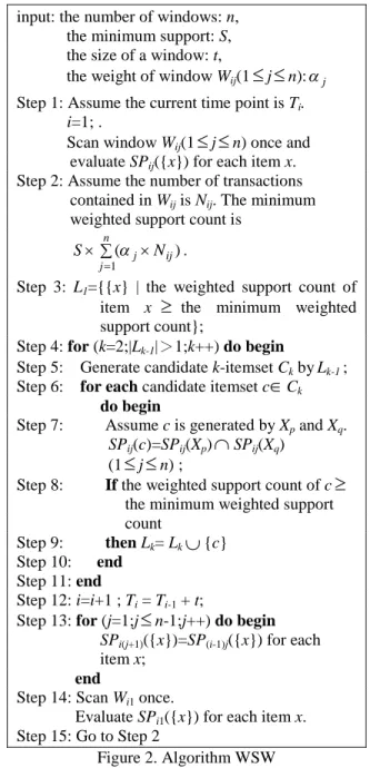
In this section, we propose algorithm WSW to discover all the frequent itemsets in the transaction data stream over weighted sliding windows.
An itemset is the set of items. If the weighted support count of an itemset is greater than or equal to the minimum weighted support count, it is called a frequent itemset. An itemset of size k is called a k-itemset. Assume the number of windows is n, the size of a window is t, the current time point is Ti, and x1,x2,...,xk are items. The transactions considered are those within the time range of Tiand (Ti- n
t ). Let SPij({x1,x2,...,xk}) be the set of identifiers of transactions containing itemset {x1,x2,...,xk} in window Wij(1jn)andj
the weight of Wij. |SPij({x1,x2,...,xk})| represents
the number of transaction identifiers in
SPij({x1,x2,...,xk}). Definition 1: If 1 n j
|SPij ({x1,x2,...,xk})|
j isgreater than or equal to the minimum weighted support count, {x1,x2,...,xk} is a frequent k-itemset。
Lemma 1:If itemset {x1,x2,...,xk} is a frequent
k-itemset, then any proper subset of {x1,x2,...,xk} is also a frequent itemset.
Similar to the method of Apriori[3], we use frequent (k-1)-itemsets to generate candidate
k-itemsets. Suppose Lk-1 is the set of all frequent
(k-1)-itemsets. X[1],X[2],…,X[k-1] represent the k-1 items in the frequent (k-1)-itemset X and X[1]<X[2]<…<X[k-1].
Definition 2: The set of candidate k-itemsets(k2),
Ck, is defined as
Ck={{Xp[1],Xp[2],…,Xp[k-1],Xq[k-1]}|XpLk-1 and XqLk-1and Xp[1]=Xq[1],
Xp[2]=Xq[2], …,and Xp[k-2]=Xq[k-2],
and Xp[k-1]<Xq[k-1]}
Different from the method of Apriori, the database is scanned only once. When a candidate itemset is generated, we can determine whether it is a frequent itemset or not by evaluating its SPij value. The detailed algorithm is shown in Figure 2. Besides, we can easily maintain all the frequent itemsets by WSW algorithm. For example, consider Figure 1. Assume we have all the frequent itemsets in window W1jat time point T1.
At time point T2, for each item x, SP24({x}) = SP13({x}), SP23({x}) = SP12({x}), SP22({x}) = SP11({x}). We only need to scan the data in W21
once in order to get SP21({x}). Once SP2jvalue of
each item is obtained, all the frequent 1-itemsets input: the number of windows: n,
the minimum support: S, the size of a window: t,
the weight of window Wij(1
j
n):jStep 1: Assume the current time point is Ti.
i=1; .
Scan window Wij(1
j
n) once and evaluate SPij({x}) for each item x. Step 2: Assume the number of transactionscontained in Wijis Nij. The minimum weighted support count is
n j ij j N S 1 ) ( .
Step 3: L1={{x} | the weighted support count of item x
the minimum weighted support count};Step 4: for (k=2;|Lk-1|>1;k++) do begin
Step 5: Generate candidate k-itemset Ckby Lk-1; Step 6: for each candidate itemset c
Ckdo begin
Step 7: Assume c is generated by Xpand Xq.
SPij(c)=SPij(Xp)
SPij(Xq) (1
j
n) ;Step 8: If the weighted support count of c
the minimum weighted support count
Step 9: then Lk= Lk
{c} Step 10: endStep 11: end
Step 12: i=i+1 ; Ti= Ti-1+ t;
Step 13: for (j=1;j
n-1;j++) do begin SPi(j+1)({x})=SP(i-1)j({x}) for eachitem x;
end
Step 14: Scan Wi1once.
Evaluate SPi1({x}) for each item x. Step 15: Go to Step 2
can be generated. According to Step 4 in the algorithm, we can discover all the frequent
k-itemsets (k2) at time point T2.
Figure 3. Algorithm WSW-Imp
4. An Improved Algorithm WSW-Imp
In this section, we propose a technique to improve the efficiency of algorithm WSW. Assume the number of windows is n, the current time point is Ti and the weight of window
Wij(1jn) is j.
Let Xp and Xq be frequent (k-1)-itemsets. Suppose they are joined to generate a candidate
k-itemset c according to Definition 2.
Lemma 2: Let Sp and Sqbe the weighted support
counts of Xp and Xq, respectively, and Sc the weighted support count of candidate k-itemset c. Sc is less than or equal to the minimum of Spand Sq (denoted as min{Sp,Sq}).
Let S’be min{Sp,Sq} and Sm the minimum weighted support count. If the weighted support count Scof candidate k-itemset c is greater than or equal to Sm, c is a frequent k-itemset. Assume c is a frequent k-itemset. γ represents the maximum difference of the weighted support count of c and the minimum weighted support count. The initial value of γis S’Sm. According to the definition of
SPij, SPij(c)=SPij(Xp)SPij(Xq), and
|SPij(c)|min{|SPij(Xp)|,|SPij(Xq)|}. Let y be
min{|SPij(Xp)|,|SPij(Xq)|}. y-|SPij(c)| represents the difference of the maximum number and the real number of transactions containing itemset c in
window Wij. If (y-|SPij(c)|)
j > γ, then theassumption that c is a frequent itemset is contradicted. Thus the process of evaluating the weighted support count of c stops. Otherwise, if (y-|SPij(c)|)
j
γ, c may be a frequent itemset.Then the process of evaluating the weighted support count of c in the next window continues and γis updated to γ-(y-|SPij(c)|)
j. In the lastwindow, if (y-|SPij(c)|)
jis still less than orequal to γ, then itemset c is truly a frequent itemset.
Based on the above discussion, we design an improved method to reduce the time of determining whether a candidate itemset is frequent or not. In Section 3, when a candidate itemset is considered, algorithm WSW needs to evaluate its weighted support count in each window. However, the improved algorithm, called WSW-Imp as shown in Figure 3, may decide whether it is a frequent itemset or not in early windows. In other words, if we cannot decide whether it is frequent or not in the present window, then the data in the next window is considered. The process continues until the candidate itemset is judged not to be a frequent itemset or the last window is considered. Thus the number of windows needed to be considered is within the range 1 to n by algorithm WSW-Imp.
We replace Step 7 ~ Step 9 in algorithm WSW with these steps in Figure 3. The initial value of
flag is 0, indicating that itemset c may be a
frequent itemset. When flag becomes -1, it represents that itemset c is not a frequent itemset. Algorithm WSW-Imp may gain better performance by reducing the number of windows to be considered.
5. Experimental Results
To assess the performance of WSW and WSW-Imp, we conducted several experiments on 1.73GHz Pentium-M PC machine with 1024 MB memory running on Windows XP Professional. All the programs are implemented using Microsoft Visual C++ Version 6.0. The method used to generate synthetic transactions is similar to the one used in [3]. Table 1 summarizes the parameters used in the experiments. The dataset is generated by setting N=1,000 and |L|=2,000. We use Ta.Ib.Dc to represent that |T|=a, |I|=b and |D|=c×1,000.
To simulate data streams in the weighted sliding window environment, the transactions in the Assume the candidate itemset c is generated by
frequent itemsets Xpand Xq;
flag = 0; j = 1; Sc= 0;
= S’- Sm; Step 1: while (flag=0 and j
n) do {// n is the number of windows Step 2: SPij(c)= SPij(Xp)SPij(Xq);
Step 3: y = min{|SPij(Xp)|,|SPij(Xq)|}; Step 4: if ((y-|SPij(c)|)
j> γ)thenStep 5: flag = -1
// It indicates that c is not a frequent itemset. Step 6: else {Sc=Sc+|SPij(c)|
j;γ= γ-(y-|SPij(c)|)
j;Step 7: j++; }} //Go to Step 1 for
evaluating the weighted support count of c in the next window.
synthetic data are processed in sequence. For simplicity, we assume that the number of transactions in each window is the same. In the following experiments, the number of windows is 4 and the weights for windows w1, w2, w3and w4
are 0.4, 0.3, 0.2 and 0.1, respectively, where w1is
the window closest to the current moment.
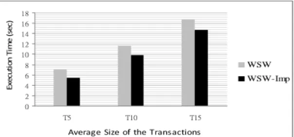
Figure 4 and Figure 5 compare the efficiency of algorithms WSW and WSW-Imp. The total number of transactions is 100K and the number of transactions in each window is 10K. (We call it the window size in experiments.) Because the number of windows is 4, the number of time points for mining is 7. The execution time in the experiment is the total execution time at seven different time points. Figure 4 shows the execution times for WSW and WSW-Imp, respectively, over various minimum supports. We can see that as the minimum support decreases, the superiority of WSW-Imp is more apparent. In Figure 5, the minimum support is 0.5%. It can be seen that the execution times for these two algorithms grow when the average size of transactions increases. However, WSW-Imp is still superior to WSW in all the cases.
Table 1. Parameters
Parameter Description
N Number of items
L Number of maximal potentially frequent itemsets
D Number of transactions T Average size of the
transactions
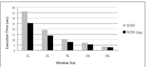
I Average size of the maximal potentially frequent itemsets In the scale-up experiment of Figure 6, the minimum support is 0.1%. It shows that the average ratio of WSW-Imp outperforming WSW maintains about 12% in all the cases. Figure 7 shows the effect of various window sizes from 1K to 20K transactions. The minimum support is 0.5%. It can be seen that when the window size increases, the difference of the execution times for WSW and WSW-Imp decreases. This is because when the window size is small, the number of transactions containing frequent itemsets in each window is small. Thus, the probability of judging a candidate itemset to be not a frequent itemset at early windows is high. In general, the performance of WSW-Imp is still better than that of WSW.
6. Conclusions
In this paper, we propose the framework of the weighted sliding windows for data stream mining. Based on the model, users can specify the number of windows, the size of a window, and the weight for each window. Thus, a more significant data section can be assigned a higher weight, which will make the mining result closer to user’s requirements. Based on the weighted sliding window model, an efficient single pass algorithm, WSW, is developed to discover all the frequent itemsets from data streams. By data characteristics, an improved algorithm, WSW-Imp, is explored to further reduce the time of deciding whether a candidate itemset is frequent or not. Experimental results show that the performance of WSW-Imp significantly outperforms that of WSW over weighted sliding windows.
0 5 10 15 20 25 30 35 40 0.1 0.2 0.3 0.4 0.5 0.6 0.7 0.8 0.9 1 Minimum Support (%) Ex ec ut io n Ti m e (s ec ) WSW WSW-Imp
Figure 4. Execution times of WSW and WSW-Imp over various minimum supports (T5.I4.D100)
0 2 4 6 8 10 12 14 16 18 T5 T10 T15
Average Size of the Transactions
Ex ec ut io n Ti m e (s ec ) WSW WSW-Imp
Figure 5. Execution times of WSW and WSW-Imp under various average sizes of transactions (I4.D100) 0 20 40 60 80 100 120 140 160 180 200 100K 150K 200K 250K 300K 350K Number of Transactions Ex ec ut io n Ti m e (s ec ) WSW WSW-Imp
Figure 6. Execution times of WSW and WSW-Imp when the database size increases (T5.I4)
0 5 10 15 20 25 30 35 40 1K 2K 5K 10K 20k Window Size Ex ec ut io n Ti m e (s ec ) WSW WSW-Imp
Figure 7. Execution times of WSW and WSW-Imp under various window sizes (T5.I4.D100)
References
[1] R. Agrawal, S. Ghosh, T. Imielinski, B. Iyer, and A. Swami, “An Interval Classifier for Database Mining Applications,”Proceedings
of the VLDB Conference, pp.560-573, 1992.
[2] R. Agrawal and R. Srikant,“Fast Algorithms for Mining Association Rules,”Proceedings of
the VLDB Conference, pp.487-499, 1994.
[3] R. Agrawal and R. Srikant, “Mining Sequential Patterns,”Proceedings of IEEE International
Conference on Data Engineering, 1995.
[4] C. Aggarwal, “Data Streams: Models and Algorithms,”Ed. Charu Aggarwal, Springer, 2007.
[5] J.H. Chang and W.S. Lee, “Finding Recent Frequent Itemsets Adaptively over Online Data Streams,” Proceedings of ACM SIGKDD, pp.487-492, 2003.
[6] Y. Chi, H. Wang, P.S. Yu and R.R. Muntz, “Catch the moment: Maintaining closed frequent itemsets over a data stream sliding window,”Knowledge and Information Systems vol. 10, no. 3, pp.265–294, 2006.
[7] P. Domingos and G. Hulten, “Mining High-Speed Data Streams,” Proceedings of
ACM SIGKDD, pp.71-80, 2000.
[8] W. Fan, Y. Huang, H. Wang and P.S. Yu, “Active Mining of Data Streams,”
Proceedings of SIAM International Conference on Data Mining, 2004.
[9] F.J. Ferrer-Troyano, J.S. Aguilar-Ruiz and J.C. Riquelme, “Incremental Rule Learning based on Example Nearness from Numerical Data Streams,”Proceedings of ACM Symposium on
Applied Computing, pp.568-572, 2005.
[10] C. Giannella, J. Han, J. Pei, X. Yan and P.S. Yu, “Mining Frequent Patterns in Data Streams at Multiple Time Granularities,”H. Kargupta,
A. Joshi, K. Sivakumar, and Y. Yesha (eds.),
Next Generation Data Mining, pp.191-210.
2003.
[11] J. Han, J. Pei and Y. Yin, “Mining Frequent Patterns without Candidate Generation,”
Proceedings of ACM SIGMOD, pp.1-12, 2000.
[12] C.C. Ho, H.F. Li, F.F. Kuo and S.Y. Lee, “Incremental Mining of Sequential Patterns over a Stream Sliding Window,”Proceedings
of IEEE International Workshop on Mining Evolving and Streaming Data, 2006.
[13] C. Jin, W. Qian, C. Sha, J.X. Yu and A. Zhou, “Dynamically Maintaining Frequent Items over a Data Stream,” Proceedings of the
Information and Knowledge Management,
2003.
[14] Y.N. Law, H. Wang and C. Zaniolo, “Query Languages and Data Models for Database Sequences and Data Streams,”Proceedings of
the VLDB Conference, 2004.
[15] G. Manku and R. Motwani, “Approximate Frequency Counts over Data Streams,”
Proceedings of the VLDB Conference,
pp.346-357, 2002.
[16] S. Qin, W. Qian and A. Zhou, “Approximately Processing Multi-granularity Aggregate Queries over a Data Stream,”
Proceedings of the International Conference on Data Engineering, 2006.
[17] B. Saha, M. Lazarescu and S. Venkatesh, “Infrequent Item Mining in Multiple Data Streams,” Proceedings of the International
Conference on Data Mining Workshops,
pp.569-574, 2007.
[18] P.S.M. Tsai and C.M. Chen, “Discovering Knowledge from Large Databases Using Prestored Information,”Information Systems, vol. 26, no. 1, pp.1-14, 2001.
[19] P.S.M. Tsai and C.M. Chen, “Mining Interesting Association Rules from Customer Databases and Transaction Databases,”
Information Systems, vol. 29, pp.685-696,
2004.
[20] Y. Zhu and D. Shasha, “StartStream: Statistical Monitoring of Thousands of Data Streams in Real Time,”Proceedings of the