CONSTRAINED OPTIMIZATION OF ACTIVE NOISE-CONTROL SYSTEMS IN ENCLOSURES

Constrained optimization of active noise control systems

in enclosures

T. C. Yang and C. H. Tseng

Department of Mechanical Engineering, National Chiao Tung University, Hsinchu 30050, Taiwan, Republic of China

S. F. Ling

School of Mechanical and Production Engineering, Nanyang Technological University, Singapore 2263

(Received 26 July 1993; accepted for publication 17 January 1994)

An effective software design tool is proposed for solving active noise control problems associated with constraints in which the complex strength and location of the secondary source of an active noise control system in an enclosed space are simultaneously optimized. The boundary element method is adopted to evaluate the sound field in enclosures. Furthermore, the boundary used could be of pressure, velocity, or impedance; in addition, the primary source may be at an arbitrary position. An optimizer based on sequential quadratic programming is selected for its accuracy, efficiency, and reliability. Bounds for design variables and proper constraints on the sound field and secondary source can be specified as required. The powerfulness of the proposed tool is demonstrated by optimizing an active control system for an enclosure. For a rectangular cavity, the optimal location of the secondary source is confirmed by observed simulations as always forming a dipole with the primary source situated at off-resonance excitations and subsequently approaching a mirror image position of the primary source at resonance excitations. The optimal location of the controller is found to change with varied upper bounds of the strength of the secondary source. These findings show a discrepancy from those reported in previous researches based on an unconstrained formulation. Sensitivity analysis at the optimum is also included to provide information of practical concern for implementing optimized active noise control systems.

PACS numbers: 43.50.Ki, 43.50.Jh, 43.55.Ka

INTRODUCTION

In enclosed spaces, although excellent noise control performance is attainable by passive means, such as using sound-absorbing materials, the cost becomes high and per- formance is significantly degraded when the acoustic wave- lengths of the noise source are comparable in size with the dimensions of the enclosure, especially below Schroeder

frequency.

• Active noise

control (ANC), on the other

hand, is most effective in noise reduction in the relatively low-frequency range. Physically, ANC is the canceling of a sound wave by adding a phase-inversed sound wave. Meth- ods of active noise attenuation primarily fall into two categoriesmreduction of the noise level in a specified re-

gion

or direction

2 and reduction

of total

noise

power.

3 The

history of and recent advances in ANC are reviewed in the

excellent

survey

papers

of Warnaka,

4 Leitch

and Tokhi,

5

and Stevens

and Ahuja.

6

Previous

studies

of optimization

of ANC

TM in an en-

closed space or exterior free space have formulated an un- constrained problem, where the optimal solutions can be analytically derived from either optimality or Kuhn-

Tucker conditions.

• However,

economic

factors

also re-

optimization

model

may

be worthwhile.

12

Similar

work

on

actuator

placement

with constraints

by Clark

and

Fuller

13

is a suitable example for active structural acoustic control (ASAC). Once the constraints are introduced, the strategy and scheme for solving the constrained optimization prob- lem may be relatively different from those techniques ap- plied toward solving the unconstrained problem.

Modal summation, the finite element method (FEM),

and the boundary element method (BEM) have been em- ployed in simulating the sound field for enclosed spaces and all these methods are satisfactory predictors. The BEM can handle various kinds of boundary properties

more easily than other methods, in addition to having ad-

vantages

over

the FEM in acoustic

applications.

TM

Hence,

in the present study the BEM is utilized in this study for evaluating the sound field in enclosures.

A design tool that integrates the numerical acoustical analysis of BEM with an optimizer based on sequential quadratic programming (SQP) is proposed in this paper for optimizing the design of ANC systems in enclosed spaces. The complex strength (magnitude and phase) of the secondary source has normally been obtained in previ- ous studies via the fixed position. In the present study, however, both the complex strength and location of the secondary source are simultaneously considered in the op- timization formulation, which is apparently a more realis- tic approach to the design of ANC systems in enclosures.

FIG. 1. Domain of acoustic system for interior Helmholtz wave equation.

The SQP is employed in this study for coping with a single- objective constrained optimization problem via a large

number of design variables as a result of its robustness and

15-18

fast convergence.

The boundary element formulation of the Helmholtz

equation is first discussed in this study so as to predict the sound field in enclosures. A constrained optimization

model is next formulated. Achieving the characteristics of

standing waves in enclosures requires choosing the total

acoustic potential energy as the general objective function, like most noise control applications. Locations and strengths of secondary sources are taken as design vari- ables in this study in• light of practical considerations.

Bounds on these variables and proper constraints are spec-

ified in forming a feasible design region. The usefulness and power of the proposed tool are demonstrated by numerical results on ANC optimization in a three-dimensional box

cavity. A design sensitivity analysis at the optimum is fi- nally discussed. This analysis provides the engineer with a

measure of what effect such variations of an optimized ANC system designs would have on the design objective after the optimization is complete.

I. BOUNDARY ELEMENT FORMULATION IN ACOUSTICS

The acoustic system in this study consists of a domain

D enclosed by a boundary B, as illustrated in Fig. 1. Vec-

tor d is the position of any point d within the domain; vector b is the boundary points b; and the location of the

primary

source

P of complex

strength

•bp

and secondary

source S of complex strength •bs within the domain are

denoted

by vectors

d

e and ds, respectively.

The indirect

BEM derived

by Chen

and Schweikert

19

and improved

by

Kipp

2ø

is applied

in this

paper

to formulate

the acoustical

proximation of Huygen's principle. The boundary is as- sumed here to be able to be replaced by a fictitious source distribution that reproduces an identical sound field in the

domain. A general form of acoustic pressure (p) and par-

ticle velocity (u) for boundary and interior points, respec-

tively, can be written via the concept of indirect BEM as

+ fo

•s(d)p*(d,•)dD, ( 1

)

u(•)

=c0a(b)

• f a

a(b)u*(b,•)dB

+ fo

(2)

where a(b) represents the fictitious source density function

at the boundary

points,

ca is an integration

constant

2• that

copes with the integral singularities, and • is a dummy variable representing boundary or interior points. The fun- damental pressure solution p* is the free space Green's function

p*( b,ff

) = ( 1/ I b-ff l )e -jlo-gl,

(3)

which satisfies

(v2 + k2)p, (o,g)

=

( 4 )

where k is the wave number and 6 is the Dirac delta func-

tion. The fundamental velocity solution u* can be related

to p* by Euler's

equation,

p au/at

= -Vp, 22

where

p is the

The indirect BEM is numerically implemented by ap-

plying a linear rectangular incompatible element to dis-

cretize the boundary. The domain integral for a point

sound source can be treated as a Dirac function multiplied by the source strength. Thus the integral exists only at the source point. Equations (1) and (2) are rewritten as

p(bi)= •

a(bj)p*(bj,bi)dBj

+

+

(dsm,O),

(5)

u(bi)--coa(bi)

+ •

a(bj)u*(bj,bi)dBj

+

+ smU*

(dsm,O),

6)

where

n e, ne, and ns are the number

of elements,

primary

sources,

and secondary

sources,

respectively;

Bj is the jth

Boundary conditions in terms of impedance may also be modeled via this method. For a locally reacting bound-

ary, the specific

acoustic

impedance

at b i is given

by

22

z(b•) =p(b•)/u(b•). (7)

A system of ne equations for the ne unknown a's is obtained by writing Eqs. (5), (6), and/or (7) for each

element according to the given boundary conditions. Thus

the ge. neral matrix form for the equations of the system can

be compactly written as

A•r-•- P•bo-•- S•bs-- a, (8)

where a contains the values of the boundary conditions, and A, P, and S can be derived from Eqs. (5), (6), or (7) according to the given boundary conditions. Once the fic- titious source a is solved, Eqs. (5) and (6) are again uti- lized in finding the acoustic pressure and particle velocity of domain points to be interested, in which the variable of boundary points bi is replaced by domain points di.

II. CONSTRAINED OPTIMIZATION MODEL

The general mathematical model for the nonlinear single-objective constrained optimization problem consid- ered here is of the following form.

Find a set of design variables x-(x•,x2,...,Xn) that minimizes an objective function

f(x), (9)

subject to the constraints

hi(x) =0, i= 1,2,...,neql,

(10)

gj (x) < 0, j = 1,2,...,niq

l,

( 11 )

where

neq

I and niq

! are the number

of equality

and inequal-

Xil<Xi<Xiu , i= 1,2 .... ,n. (12) Both the objective function f(x) and the constraints hi(x )

and

gj (x) are assumed

to be continuous

differentiable.

The

(12). Three elements are included in a well-defined math-

ematical statement of optimization•design variables, the objective function, and design constraints. The primary purpose of this study lies in forming a constrained optimi- zation problem that optimizes the complex strength and location of the secondary source for the design of ANC systems in enclosures. Additionally, the acoustic behavior of secondary sources via appropriate constraints is also investigated.

A. Optimization strategy and formulation

As noted in the Introduction, in previous work the complex strength (for example, input voltage and phase) of the secondary source was optimized under a fixed posi- tion. In this present study, however, both location ds and complex strength •b s of the secondary source are chosen as design variables because of practical considerations. Loca- tion ds is represented here by coordinates of x, y, and z, and complex strength •bs is replaced by magnitude •b and phase 0. If the primary source is known and controlled by the secondary source, the acoustic pressure at field points of the enclosure at a given frequency can then be written as

pi=pi(x,y,z,

qb,O), i = 1,2,...,nfp;

( 13

)

where

nfp

is the number

of field points

to be evaluated.

control, on the other hand, is characterized by an attenu-

ation of the noise level throughout the cavity. Each of these strategies employs an acoustic secondary source, which, for practical purposes, would typically be loudspeakers. The primary source of sound is assumed to have a harmonic waveform and can be positioned anywhere in the cavity; in

addition, the secondary source can be driven at the same

frequency. The position and strength of the secondary source are varied for minimizing the objective function, which is implemented in this paper by the total acoustic potential energy of the control volume. The objective func- tion for various control strategies can always be formulated

as

1 • Ip(x,y,z,

ck,o)]2

dV,

(14)

•--4-• v

where c and V represent the speed of sound and the control volume, respectively. The • can notably be measured only by ideal distributed sensors, which may not be practical for application purposes. In practice, a reasonable number of acoustic pickups (e.g., microphones) are uniformly distrib- uwd throughout the cavity to collect the response utilized in fo•ulating the discrete form of the objective function. As can be seen from Eq. (15), this fo• becomes ve• •arly proportional to the continuous form of Eq. (14)

and is used in the numerical simulation. The control vol-

ume V can notably be taken out of the summation only if the error sensors are uniformly dist•buted throughout the cavity. Otherwise, the contribution of each sensor must be weighted'

•--4P

c2

i=

•

'

All engineering systems are designed to perfore within a given set of constraints, which includes limitations on resources, material failure, response of the system, and

member

sizes.

Two ,types

of constraints

are introduced

in

low.

1. Bounds on design variables The bounds are

Xi•Xi•Xu, i=l,2,...,ns, (16) Yl<Yi<Yu, i= 1,2,...,ns, (17) zl<zi<Zu , i= 1,2 .... ,ns, (18) qbi<qbi<qbu, i= 1,2,...,ns, (19) O•,<O•<Ou, i= 1,2,...,ns, (20)

where the subscripts I and u indicate the lower and upper bound of the design variables, respectively.

2. Inequality constraints

The secondary source clearly has the possibility of ap- proaching the position of the primary source, that is, if no constraint is imposed on the relative location of the pri- mary and secondary sources. This should be avoided in light of practical concerns. Also, for multiple control sources the spaces between the control sources must be reserved for convenient installation. Constraints of Eqs. (21 ) and (22), which express the permissible spaces for installing the ANC system, are therefore required from an engineering prospective:

i= 1,2,...,np

and j= 1,2

.... ,ns,

j=i+l,i+2,...,ns, (22)

where

6ps

and 6ss

are the allowable

distances

between

the

SPL at (xj,yj,zj)--Lp<O, j= 1,2,...,nspl; (23)

where

Lp and nsp

1 are the specified

SPL and number

of

assigned locations, respectively.

In summary, the design optimization model presented here finds the location (x,y,z) and complex strength (•b,0) of the secondary source to minimize the objective function, the total acoustic potential energy of Eq. (15), subject to the constraints of Eqs. (16)-(23).

B. Optimization scheme and algorithm

Multiple minima are basically presented in the feasible domain of the preceding optimization problem along with a number of numerical nonlinear programming (NLP) methods capable of solving it. The sequential quadratic programming (SQP) is, however, selected in this study

because

of its convergence

and robustness.

•5-18

The SQP

algorithm is importantly a generalized gradient-descent op- timization method, and subsequently converges to a local

rather

than global

optimum.

TM

A conceptual

flow chart

of

the SQP algorithm is depicted in Fig. 2, which reflects the characteristics of the direct iterative optimization method (i.e., definition of a subproblem). This optimization method solves the subproblem to give the direction of de- sign improvement, and a step size along the search direc- tion. The steps of the algorithm are summarized as follows.

Step 1. Initial state: Set k=0. Estimate initial values of

design

variables

as x ©. Select

an appropriate

initial

value

for the penalty parameter R =R 0 > 0, and two small num- bers that define the permissible constraint violation el and convergence parameter e2, respectively.

Design Update x(k+0= x00+ c•kAx 00 k=k+l Initialization setk=0 Hessian H(% Identity I

guess an initial x (o)

Search Direction (Ax 00)

solve QP subproblem

Step Size

line search

updated

by

BFGS

formula

I

FIG. 2. Conceptual flow chart of the SQP algorithm.

Step

2. Search

direction:

The direction

Ax

(k) of the

iterative

formula

x (k+

l) =x(•) +a•Ax(•) is determined

by

solving a quadratic programming (QP) subproblem, de-

fined as finding

an n vector of Ax

(•) to minimize

{Vf(x(k)),Ax(•)}+0.5(Ax(•),HAx(•)),

subject to the

constraints

hi(x

(•)) + {Vhi(x(k)),Ax(•)}

= 0, gj(x

(•))

q-(•7gj(x

(k) ),Ax(k))•<0,

and

Xil<X

(k)

i-•-

Ax(k)

<Xiu,

where

(A, B) = A rB. H is a positive

definite

approximation

of the

is defined

as L(x,/•)=f(x) -+-•ihi(x) q-•jgj(x).

Step 3. Convergence criteria: If the maximum con-

straint

violation

V(x ©) is less

than

a given

accuracy

(say,

El), and the convergence

parameter

I

The V(x) is defined as max{O, I h (x) I ,-..,

Ihn'(x) I,Ign'+a(x)I,...,Ih•(x)I}, where n' = neq

l and

N = neq l q- niq l.

Step 4. Penalty parameter: Calculate r=•; I,1, where

the Lagrange multipliers/•i are obtained from the solution of the previous QP subproblem, and check the condition of

R•>•

r. If it is violated,

let Rk= 2r. Otherwise,

let R•= Rk_ 1.

The penalty parameter R is chosen by the compromise between the constraint correction and the algorithm effi- ciency. The procedure applied here functions quite effec-

tively.

Step 5. Step size: To find a• of the iterative formula

x(•+l)=x (•) +akAx

©. A line search

is used

and the step

size

a• is chosen

as 0.5

J, with J as the smallest

positive

integer to satisfy the descent condition of descent function cp(x)=f(x)+RV(x) and 0</•< 1. The descent function is introduced because of its simplicity and

•

Optimization Inpu•l'•

... . ,,

•,• •.//•d',., ,•• ... •,•:•..•,:,.,•, ..

•'•••'

... • User-su,, lind •nct•ons • •' ...

•c• •'•..•-,•..•,• .... • ... • . ß

•.' % :•.,,?f • .(,• ' SO•LD

• Read input •ta • ' • , ' • "• •"

• •,• CUSERMF • • O•E•

• _. .

• •

_....

• •un• Element

. ,, • .. •.•

Output file

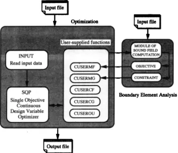
FIG. 3. Architectural framework of the proposed design tool, where CUSœRXXs are user-supplied functions. CUSœRMF and CUSœRMG compute the value of objective and constraint functions, respectively. CUSERCF and CUSERCG calculate the gradient of objective and con- straint functions, respectively. CUSœROU can provide additional data for

verification.

success in solving a large number of engineering design

problems.

•7 Additionally,

this function

also

has

the prop-

original objective function.

Step 6. Hessian update: A number of procedures can be applied towards updating the Hessian matrix H. The

BFGS (Broyden-Fletcher-Goldfard-Shanno) form-

ula,

23'24

considered

as a better

strategy,

•8 is selected

in this

paper for guaranteeing a positive definite updated Hessian.

If k=0, let H © be an identity

matrix

I.

Step Z New iteration: Set k=k+ 1, update the design

as XCk+•)=XCk)+akAXCk),

and

go to Step

2.

A certain number of numerical experiences are re- quired in implementing the scheme in terms of robustness and efficiency, despite the fact that the SQP algorithm is apparently well defined. Refer to the research of Tseng and Arora •7 for details. All the elements of the constrained optimization model defined in this paper are incorporated into an architectural framework for the proposed design tool, as exhibited in Fig. 3. The communication between the BEM acoustical analysis and the SQP optimization during the solution procedure is illustrated in this archi-

tectural framework.

III. NUMERICAL SIMULATIONS AND DISCUSSION

The active noise controllers often attempt canceling out a group of related or nonrelated harmonics during practical application by employing the same set of control sources positioned at the same locations in the cavity. Only a single harmonic line is considered in this study since this is sufficient for demonstrating the advantages afforded with the proposed optimization. In linear acoustics, however, the principle of superposition can be applied to compute

the sound field. This sound field then is further utilized in

forming the defined objective function and in optimizing both complex strengths and positions for the control of several harmonic lines in the proposed optimization proce- dure. This procedure is simply implemented by adding an iterative loop in the sound field computation module of boundary element analysis (in the right side of Fig. 3). Also, in practical applications the primary source is often outside the cavity (e.g., engine in a car or propellers in an aircraft). In coping with these applications, the appropri- ate analytical or measuring tool should be utilized first to investigate the impact of outside sources on the boundaries of the cavity (e.g., finding the equivalent primary sources distributed on the boundaries or inside the cavity). The BEM can accurately predict the acoustical field of the cav- ity if the characteristics of a boundary and/or the equiva- lent primary sources are well known. The primary sources are assumed here, for brevity's sake, as known and are positioned randomly anywhere in the cavity.

A geometrical configuration of a box type is most com- mon for medium or small rooms. Consequently, the nu- merical simulations presented here are based on a rectan- gular enclosure with dimensions of 4 m X 5 m X 3 m. The

grid points

that determine

the squared

acoustic

pressure

p2

z= 1.2 m and 1.6 m (approximately the head height of a person seated in the enclosure). A frequency ranging from 30 to 200 Hz is selected to compensate for the limited accuracy of the BEM in determining the lower bound and the constraint of the Schroeder cutoff frequency for the upper bound. The primary and secondary sources are as- sumed here to vibrate with the same frequency and are in a steady state. For cases studied below, the acoustic system has rigid boundaries (i.e., the acoustic velocity normal to

boundaries is zero).

A. Optimal location of secondary source versus frequency

No clear evidence is available in the previous litera- ture, which indicates a specific qualitative relation between the optimal placement of the secondary source and the excitation frequency of the primary source, especially in the three-dimensional cavity. Therefore, this section is de- voted to discovering such a relation. Two caseswone with single and one with multiple primary sources--are inves- tigated. The excitation frequency of the primary source is divided into two categorieswoff-resonance and resonance

excitations of the enclosure. For resonance excitations of the enclosure, six modes are studied: mode (0,1,0)=34.3 Hz, .(1,0,0)=42.9 Hz, (0,0,1) =57.2 Hz, (0,2,0)=68.9

Hz, (2,0,0)=86.1 Hz, and (2,2,0)= 110.6 Hz. Typical re-

sults obtained for these cases are discussed below. 1. Enclosure with single primary source

A primary

source

P• of volume

velocity

1 m3/s

is po-

sitioned close to one corner (3.8,4.5,2.5) of the cavity with a harmonic excitation. The design bounds and constraints,

respectively,

are 0< •bs<

1 m3/s,

- 180<

Os<

180

deg,

0<x< 4

m, 0<y<5 m, 0<z<3 m, 0.1 m<ld-dsl, and SPL at

z I I I Pl S1 0

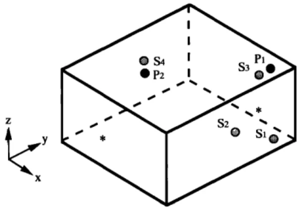
FIG. 4. Schematic diagram of ANC in the enclosure with single primary source. Primary source P1 is positioned at (3.8,4.5,2.5). Optimal candi- date locations of secondary source are as follows: S1=(3.8,4.4,2.5), S2= (3.8,4.5,0.5), and S3= (0.2,0.5,0.5). The asterisk represents the po- sition of specified SPL.

110

I o o

' ' •"

no

control

:,,,

::

: ,,

g

'd ,, ::

',: •

"

• 8o

•; ;'

•

"

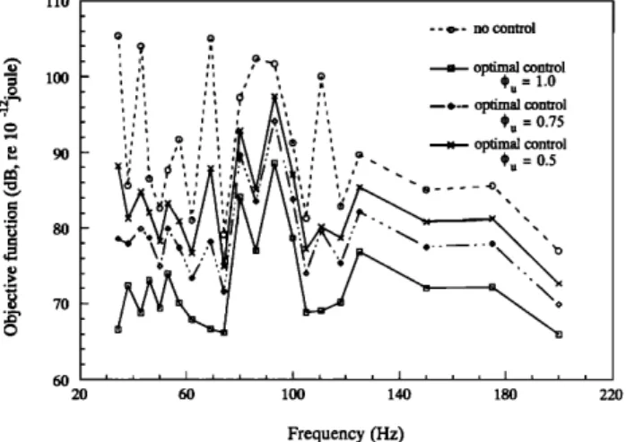
FIG. 5. Objective function as a function of frequency for the case of rectangular enclosure with single primary source (Secs. IIIA 1 and III B). •bu is the upper bound of the strength of the secondary source.

trarily chosen for illustrative purposes. At off-resonances, the optimal secondary source always approaches closely a position of $1 = (3.8,4.4,2.5) with an antiphase (i.e., -- 180 deg), where it approximately forms a dipole with the pri- mary source P1. For a cavity of simple geometrical config- uration (e.g., the rectangular ,•-,• used i, t•i• ••-• t• position of maximum acoustic pressure (globally) is pri- marily located in the vicinity of the primary source at off- resonance excitations. Via this simple geometrical con- straint, the optimal secondary source positioned in or close to this place can effectively attenuate the noise as indicated by the above results. More than one position of peak acous- tic pressure (locally) is available in the cavity at higher excitation frequencies of the primary source [but still below the Schroeder cutoff frequency (in this example 200 Hz)].

The solution can therefore be varied from different initial

designs in light of the algorithm searching for the local minimum. The optimization solutions shown here and af-

ter are selected from the better one of various initial con-

ditions. However, a totally different situation is obtained at resonances of the enclosure. The optimal secondary source of modes (0,1,0), (1,0,0), and (2,0,0) approaches S2= (3.8,4.5,0.5), a mirror image position of P• along an edge, and it approaches S3 = (0.2,0.5,0.5), a mirror image position of P• along a diagonal, for modes of (0,2,0) and

(2,2,0). The optimal secondary source is, however, patched to S• = (3.8,4.4,2.5) for mode (0,0,1 ). Physically, the results for a cavity with a simple geometrical configu- ration can be related to the position of the primary source, and the shape of sound field in the enclosure, in which it is almost of geometrical symmetry and the positions of peak acoustic pressure are close to the boundaries. The relative positions of P•, S•, S2, and S3 are shown in Fig. 4. The complex strength of the optimal secondary source in each

case

is of volume

velocity

1 m3/s

and

phase

-- 180

deg

shift

relative to the primary source. This knowledge of the dis- tribution of the optimal secondary source in the frequency range of interest suggests that a sufficient guideline for setting up an ANC system lies in either attempting an edge or diagonal mirror image position of the primary source for

resonance excitation or placing the secondary source close to the primary source for off-resonance excitation. The mir- ror image strategy is similar to that of efficient coupling into the appropriate mode, as advocated by Bullmore

et al.

25

in a two-dimensional

cavity,

in which

the

placement

of the secondary source is based on the shape analysis of sound field before control. However, for cavities of irregu- lar boundaries it is not easy to predict the positions of peak acoustic pressures in advance. Therefore, an optimization procedure optimizing the positions and complex strengths of the control sources at the same time makes the tool very attractive for practical work in active noise control. Note that this rule is generally valid for simple cavities with geometrical constraints among the sound sources. Figure 5 illustrates that the optimal controller performs well at fre- quencies below 100 Hz, where reduction of total acoustic potential energy is more than 15 dB. All of the constraints are satisfied in these simulations and the SPL at the spec- ified positions is below 90 dB, which implies that this con-

straint is inactive.

2. Enclosure with multiple primary sources

Two primary sources, P1 and P2 of volume velocity 1

m3/s,

in-phase,

and

the same

excitation

frequency,

are po-

sitioned close to (3.8,4.5,2.5) and (0.2,2.5,1.5), respec- tively. The one-on-one approach is chosen as the control technique that attenuates the noise level in a specified re- gion; that is, each primary source is controlled by a corre- sponding secondary source. The design bounds are

O<•bsl,•bs2<l

m3/s,

--180<0s],0s2<180

deg,

O<x],x2<4

m,

O<y•,y2<5 m, and O<z•,z2<3 m, and the constraints are

O.l m<ld.o•-ds•

I, O.l m<ld•--ds2

I, 0.1 m<ld•2--dsl

I,

0.1 m< I d2-ds2 I, 0.1 m< I ds-d2 I, and SPL at positions

of ( 1.5,1.2,1.4) and (3.2,4,1.6) < 100 dB, respectively. At resonance excitations of the enclosure, the optimal locations of the secondary sources are at S1 = (3.8,4.5,0.5) and S2 = (3.8,2.5,1.5) for modes of (0,1,0) and (2,0,0); meanwhile, for other modes they change to S3 = ( 3.8,4.4,2.5 ) and S4 = (0.2,2.5,1.6). Relative positions

z I 0 S4 I p•

• p• I

S3

0

,

¸ S•.:•

FIG. 6. Schematic diagram of ANC in the enclosure with multiple pri- mary sources. Locations of primary sources P• and P2 are positioned at (3.8,4.5,2.5) and (0.2,2.5,1.5), respectively. Optimal candidate locations of secondary sources are as follows: S•---(3.8,4.5,0.5), S2= 3.8,2.5,1.5), S3-- (3.8,4.4,2.5), and S4-- (0.2,2.5,1.6). The asterisk represents the po- sition of specified SPL. 11o no control optimal control 20 60 100 140 180 220 Frequency (Hz)

FIG. 7. Objective function as a function of frequency for the case of rectangular enclosure with multiple primary sources (Sec. IIIA 2).

of S•, S2, S3, and S4 are shown in Fig. 6. The optimal

complex

strength

for all the secondary

sources

is 1 m3/s

in

magnitude and -180 deg in phase shift. Note that at res- onance excitations, the optimal locations of the secondary sources are primarily not at edge or diagonal mirror image positions of the primary sources. However, these locations tend to form a dipole with the corresponding primary source. At off-resonance excitations, the optimal locations of the secondary sources are always at S3 and S4, respec- tively, where they tend to form a dipole with the corre- sponding primary source. The same physical reasoning as in Sec. IIIA 1 can be applied on the basis of the above results. For the case of multiple primary sources, however, the sound field in the enclosure is more complex than the one of a single primary source. Additionally, its locations of maximum and/or peak acoustic pressure are highly de- pendent on the relative positions and phase differences of the primary sources. Unlike the case of a single primary source, predicting the optimal locations of the controllers would be difficult without carrying out simulations such as those described here. However, a general strategy for the placement of secondary sources for the case of multiple primary sources can still be suggested. The secondary source is first patched so as to form a dipole with the cor- responding primary source. If that does not work, one should then attempt to position the secondary source in an edge mirror position of the corresponding primary source. This is somewhat different from the strategy demonstrated in Sec. IIIA 1. The performance of the optimal ANC is verified in Fig. 7 by the reduction of the total acoustic potential energy in the control volume, where it is over 15 dB in the frequency below 110 Hz.

B. Effect of design bound

Table I compares the optimal locations of the second-

ary source at resonance excitations of the enclosure for

different upper bounds on the strength of the secondary source, •b u. The enclosure of a single primary source is again discussed here, assuming that the volume velocity of

the primary

source

is 1 m3/s.

As expected,

for the case

where

•bu>

1 m3/s

the optimal

placement

of the secondary

source

is the same

as that for the case

where

•bu

= 1 m3/s.

This is because for cavities of simple geometrical configu- ration the primary and secondary source having equal but inverse contribution can make the greatest noise reduction in a one-on-one control strategy.

For cases

of •bu

< 1 m3/s,

however,

the location

of the

optimal controller is quite different from that in the case of

•bu

= 1 m3/s.

Because

of the lack

of effective

power,

in most

situations the controller cannot be afforded with the largest

attenuation

at the position

of the case

•bu>•

1 m3/s;

as a

result, the controller converges to the other place (local minimum) by tailoring its strength. As mentioned in Sec. III A, the positions of peak acoustic pressure are in or close to the boundaries of the cavity at resonance excitations.

Hence,

for the case

of •bu

< 1 m3/s

the optimal

location

of

the secondary source is definitely in the vicinity of the

mirror

image

of the primary

source.

For •bu

< 1 m3/s

the

optimal location would generally approach a position some distance away from an edge or a diagonal mirror image position of the primary source. Furthermore, the objective function increases as •bu decreases. For example, at 34.3 Hz the optimal locations of the secondary source for •bu>• 1,

•bu=0.75, and •bu=0.5 m3/s are at (3.8,4.5,0.5),

superscript "+" indicates "in the neighborhood of." At resonances of 68.9 and 110.6 Hz, however, the optimal

controller

of •bu

< 1 m3/s

is located

in the vicinity

of the

position

of •bu>•

1 m3/s

along

with the values

of the objec-

tive

function

for •bu>•

1 m3/s

and

•bu=0.75

m3/s

being

quite

close (at least in the first decimal digit). This infers that for

•bu>/0.75

m3/s

at these

two resonances,

the objective

func-

tion is insensitive to the variation of design variables in the neighborhood of the position (0.2,0.5,0.5).

The upper bound of the strength of the secondary source having a definite impact on the optimal placement of the controller is confirmed by the above results. Also, at the optimum the magnitude •b of the secondary source reaches to •bu in most situations, where only maximum

TABLE I. Comparison of the optimal location of the secondary source with objective function at resonances of the enclosure for various upper bounds on the strength of the secondary source, •u- The superscript "+" indicates "in the neighborhood of."

Frequency •bu•

1

m3/s

•b•=0.75

m3/s

•u=0'5

m3/s

No

control

(Hz) (x,y,z) f (dB) (x,y,z) f (dB) (x,y,z) f (dB) f (dB)

34.3 (3.8,4.5,0.5) 65.3 (0.2,0.5,2.5) + 78.6 (0.2,0.5,0.5) + 88.2 105.4 42.9 (3.8,4.5,0.5) 67.5 (0.2,0.5,2.5) + 79.9 (3.8,0.5,0.5) + 84.8 103.6 57.2 (3.8,4.4,2.5) 77.4 (0.2,4.5,0.5) + 78.3 (0.2,0.5,2.5) + 80.9 92.4 68.9 (0.2,0.5,0.5) 78.2 (0.2,0.5,0.5) + 78.2 x (0.2,0.5,0.5) + 87.9 105.1 86.1 (3.8,4.5,0.5) 77.0 (3.8,0.5,0.5) + 83.6 (0.2,0.5,0.5) + 85.1 102.4 110.6 (0.2,0.5,0.5) 79.6 (0.2,0.5,0.5) + 79.6 (0.2,0.5,0.5) + 80.1 99.9

output of the controller can make the effective noise reduc- tion. The optimal phase 0 is normally either a 0 or --180 deg shift, which depends on the phase of the optimal po- sition in the sound field before control, relative to the pri- mary source. From a practical point of view, the general strategy for placement of the optimal controller obtained in Sec. IIIA must be modified if the power of the secondary source being smaller than that of the primary source is

used.

IV. SENSITIVITY ANALYSIS

Two categories of sensitivity information are generally of interest and significance during and/or after optimiza- tion of engineering systems. Parameter sensitivity analysis is to be performed if system parameters are modified after the optimization is complete. The primary objective of pa- rameter analysis lies in both estimating the sensitivity of an optimum design to some new problem parameter and pro- viding the engineer with a measure of what effect such changes would have on the design. Some useful methods, including the traditional approach based on the Kuhn- Tucker necessary conditions for optimality, are available in

Vanderplaats

and

Yoshida.

26

A systematic

sensitivity

anal-

ysis using a multiobjective optimization approach for the determination of system parameters has also recently been

proposed.

27

Another

kind of sensitivity

information

is the

first and second derivatives of objective and constraint functions on design variables, which are also referred to as the gradient and Hessian, respectively. Such information plays a key role in the search of optimal point. Most search methods require either first- or second-order information. Deriving an explicit expression for gradient and Hessian is often difficult in an engineering design optimization as a consequence of the complexity of engineering systems. Therefore, how this information can be accurately and ef-

28

ficiently obtained has been extensively investigated. One simple but extensively utilized approach is the finite differ- ence method. For a given tolerance, this approach can pro- vide an adequate approximation to either first- or second-

order derivatives.

The estimation of effects of relative small errors

present during the installation and/or operation of the op- timal controller on the optimal design is of primary con- cern in this study. Therefore, the sensitivity of objective function on design variables, i.e., position vector for instal- lation and complex strength for operation, can be practical

for required sensitivity analysis. A case of Sec. IIIA 1 is employed in demonstrating the concept of sensitivity anal- ysis described above. The required sensitivity c•f(x)/o•x for design variables x is shown in Fig. 8 at various frequencies, in which it is divided into three groups because of different dimensions for design variables. Table II is included to compensate for any misconception that has probably arisen from the fact that the sensitivity to position (x, y, and z) actually has not the same dimensions as that for strength (•b and 0). The effect of each design variable on the design objective is presented in Table II under a specified varia- tion of the optimal value. Via this information, more at- tention is drawn to those design variables that have a sig- nificant effect on design requirement in the course of installation and operation. As a result, the required opti- mum design can be correctly implemented. On the other hand, the total resulting variation of objective function can be evaluated on the basis of the deviations of design vari- ables 6x (after final setting up) by 6f=c9f/ C•X 1 •Xl +C• f /c•x 2 •X2+ ' ' ' +c• f /c•x n •X n. An optimal con- figuration is assumed to be reached if this value is within an acceptable range; otherwise, retuning of the controller is necessary. Some conclusions can be drawn from the sensi- tivity information and the effect of each design variable on the objective function given in Fig. 8 and Table II.

(i) For position components, the sensitivity with re- spect to x is generally more significant with all resonant frequencies. This implies that the x component of the po- sition of the controller demands more accuracy during in-

2000 1500 - 1000 - ß 34.3 Hz • 42.9 Hz • 57.2 Hz ß 68.9 Hz • 86.1 Hz IllIll 110.6 Hz I I I I I x y z • 0

position magnitude phase

Design variable

FIG. 8. Sensitivity analysis of the secondary source at optimum.

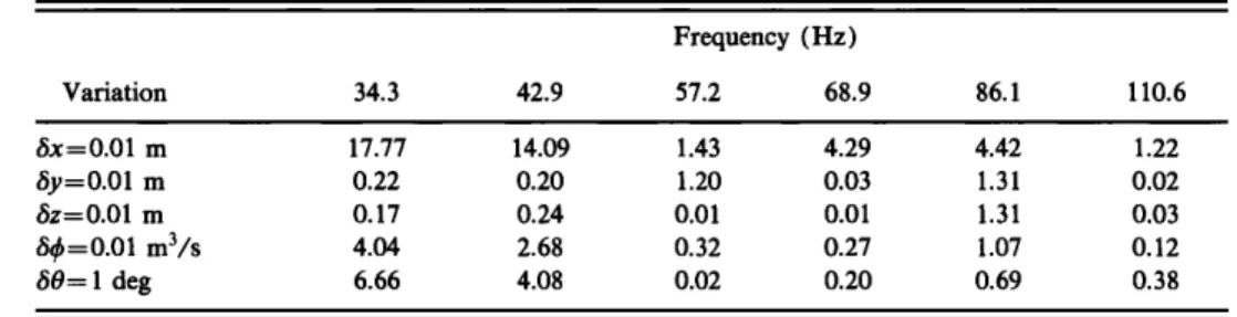
TABLE II. The effect of a small variation of design varables on the objective function at the optimum. The figures provided here represent the increase of objective function in decibels. Note that while one of design variables is varied, the other variables remain unchanged.

Frequency (Hz) Variation 34.3 42.9 57.2 68.9 86.1 110.6 •Sx=0.01 m 17.77 14.09 1.43 4.29 4.42 1.22 •Sy=0.01 m 0.22 0.20 1.20 0.03 1.31 0.02 •Sz=0.01 m 0.17 0.24 0.01 0.01 1.31 0.03 •b=0.01 m3/s 4.04 2.68 0.32 0.27 1.07 0.12 •50= 1 deg 6.66 4.08 0.02 0.20 0.69 0.38

stallation while others may allow some deviations. How- ever, the x dominate can be related to the shape of sound field in this simple cavity. At resonance excitations, the

shape of original sound field in the vicinity of the mirror image of the primary source (such as the positions of S2 and $3 in Fig. 4) is quite fiat along the y or z direction but rather steep along the x direction, especially at resonances

of 34.3 and 42.9 Hz. Hence, a small variation of •Sx with

the optimal value has a larger effect than those of •Sy and on the objective function. Also, the effect of variation •Sx at lower frequencies of 34.3 and 42.9 Hz is more crucial than that at higher frequencies, where reasoning similar to that above can be applied.

(ii) For the characteristics of the controller itself, the

given sensitivity indicates that the design objective is gen- erally insensitive to the variation of •5•b (except for 34.3 and 42.9 Hz) and •50. This sensitivity arises since the optimal placement of the secondary source is of efficient coupling into the appropriate mode, in which the design objective is primarily influenced by the positions of peak acoustic pres- sure (local minima). In light of the different dimensions of •b and 0, the combination of sensitivity analysis (Fig. 8) and the effect of design variable on the objective (Table II) is required for evaluating their influence. For example, at resonance of 34.3 Hz the sensitivity of c•f(x)/o•x for •b is substantially larger than that for 0. From Table II, a vari-

ation of •5•b=0.01

m3/s produces

a 4.04-dB

increase

of

objective function and, however, a 6.66-dB increase for the variation of •50= 1 deg. Further, if the variation is doubled, a 7.85-dB increase of objective function would occur for

/5•b=0.02

m3/s, as compared

to a 11.66-dB

increase

for

•50= 2 deg. Accurately controlling the phase of controller is difficult in application. From this point of view and the results shown above, careful tuning is thus required in set- ting up the phase of the controller.

(iii) The sensitivity with respect to x at 57.2 Hz is significantly less than that at other frequencies. In this case, the objective function is apparently insensitive with respect to all design variables. However, which factor will dominate the design? The optimal location of the second- ary source in this case can be postulated as being so close to the primary source that the former can still produce the proper approximated inversed acoustic field so as to atten-

uate the noise under a small variation of •Sx. This argument

is supported by the observation that the inequality con-

straint, which defines the allowable distance between the

primary and secondary sources, is active in this case. Fur-

ther insight into the sensitivity on the constraint could be obtained by performing a parameter sensitivity analysis with respect to parameter •Sa, i.e., the inequality constraint is changed from g(x)<0 to g(x)<•Sa. The multiobjective

optimization

approach

reported

by Tseng

and Lu 27

is sug-

gested for further details regarding the sensitivity on •Sa. A working instruction on the installation and opera- tion of the active noise control system can be drawn on the basis of the optimal design along with the above sensitivity analysis so as to guide all of the implementations.

V. CONCLUDING REMARKS

An effective software design tool was proposed in this study for solving active noise control problems associated with constraints, in which the complex strength and loca- tion of the secondary source of an active noise control system in an enclosed space are simultaneously optimized. In light of practical considerations, the design of an active noise control system in an enclosure was formulated as a constrained optimization problem but not as an uncon- strained one as proposed in previous research efforts. The approach presented above was found to be straightforward and versatile. The acoustic properties of the enclosure boundaries and the complex strength and location of the primary and secondary sources could easily be varied. The parameters assigned in the optimization scheme SQP proved effective in ensuring the scheme robust as it con- verges quickly (within a few iterations) for all the example cases. Convergence to a local minimum would also be guaranteed by this scheme for various initial designs.

This constrained optimization model was applied to- ward designing ANC systems for a rectangular cavity through computer simulations. Results indicated the opti- mal location of the secondary source generally tends to form a dipole with the primary source at off-resonance excitations and approaches a mirror image position of the primary source at resonance excitations of the enclosure. Furthermore, the optimal location of the controller was observed to change for varied rates of output powers of the secondary source, which corresponds to the upper bound of the strength of the secondary source. The effect of a small variation in •Sx being crucial was confirmed by sen- sitivity analysis at the optimum, especially at lower reso- nant frequencies. Consequently, this effect could be related to the shape of sound field in this simple cavity.

ACKNOWLEDGMENTS

The authors acknowledge the support of the National

Science Council, Taiwan, R.O.C., under Grant No.

NSC82-0401-E009-085. Review of this manuscript by T. W. Lu is also appreciated.

1T. Salava, "Acoustic load and transfer functions in rooms at low fre- quencies," J. Audio Eng. Soc. 36, 763-775 (1988).

2S. Onoda and K. Kido, "Automatic control of stationary noise by means of directivity synthesis," Proc. 6th ICA Congr. Tokyo IV, F185-

188 (1968).

3 p. A. Nelson, A. R. D. Curtis, S. J. Elliott, and A. J. Bullmore, "The minimum power output of free field point sources and the active control

of sound," J. Sound Vib. 116, 397-414 (1987).

4G. E. Warnaka, "Active attenuation of noise--The state of the art," 1982 Noise Contr. Eng. J. 18, 100-110 (1982).

5R. R. Leitch and M. O. Tokhi, "Active noise control systems," IEE

Proc. A 134, 525-546 (1987).

6 j. C. Stevens and K. K. Ahuja, "Recent advances in active noise con-

trol," AIAA J. 29, 1058-1067 (1991).

? P. A. Nelson, A. R. D. Curtis, S. J. Elliott, and A. J. Bullmore, "The active minimization of harmonic enclosed sound fields, part I: Theory,"

J. Sound Vib. 117, 1-13 (1987).

8C. G. Mollo, "A numerical method for analyzing the optimal perfor-

mance of active noise controller," M.Sc. thesis, Purdue University (1987).

9K. A. Cunefare and G. H. Koopmann, "A boundary element approach to optimization of active noise control sources on three-dimensional

structures," J. Vib. Acoust. 113, 387-394 (1991).

1øC. H. Jo and S. J. Elliott, "Active control of low frequency sound

transmission between rooms," J. Acoust. Soc. Am. 92, 1461-1472 (1992).

11j. S. Arora, Introduction to Optimum Design (McGraw-Hill, New

York, 1989).

12T. C. Yang, C. H. Tseng and B. T. Lee, "A Boundary Element and Optimization Approach for Designing of Active Noise Control Systems in Enclosures," Proc. Int. Noise Vib. Contr. Conf., St. Petersburg, Rus-

sia, 3, 269-274 (1993).

13R. L. Clark and C. R. Fuller, "Optimal placement of piezoelectric actuators and polyvinylidence fluoride error sensors in active structural acoustic control approaches," J. Acoust. Soc. Am. 92, 1521-1533

(1992).

14 p. K. Banerjee and R. Butterfield, Boundary Element Methods in En- gineering Science (McGraw-Hill, London, 1981 ).

15 K. Schittkowski, "The nonlinear programming method of Wilson, Han and Powell with an augmented Lagrangian type line search function, part I: Convergence analysis; Part II: An efficient implementation with linear least squares subproblem," Num. Meth. 38, 83-127 (1981). 16 j. Stoer, "Foundations of recursive quadratic programming methods for

solving nonlinear programs," in Proceedings of the NATO Advanced Study Institute on Computational Mathematical Programming, Bad Windshim, Germany (1984).

17 C. H. Tseng and J. S. Arora, "On implementation of computational algorithms for optimal design, part I: Preliminary investigation; Part II: Extensive numerical investigation," Int. J. Num. Meth. Eng. 26, 1365-

1402 (1988).

18C. H. Tseng and W. C. Liao, "Integrated software for multifunction optimization," M.Sc. thesis, National Chiao Tung University, R.O.C.

(1990).

19L. H. Chen and D. G. Schweikert, "Sound radiation from an arbitrary body," J. Acoust. Soc. Am. 35, 1626-1632 (1963).

20 C. R. Kipp, "Prediction of sound fields in acoustical cavities using the boundary element method," M.Sc. thesis, Purdue University (1985). 21C. A. Brebbia and S. Walker, Boundary Element Techniques in Engi-

neering (Newnes-Butterworths, London, 1980).

22 L. E. Kinsler, A. R. Frey, A. B. Coppens, and J. V. Sanders, Funda- mentals of Acoustics (Wiley, New York, 1982).

23M. J. D. Powell, "The convergence of variable metric methods for nonlinearly constrained optimization calculations," in Nonlinear Pro- gramming, Vol. 3, edited by O. L. Mangasarian et al. (Academic, New

York, 1978).

24 p. B. Thanedar, J. S. Arora, and C. H. Tseng, "A hybrid optimization method and its role in computer-aided design," Comp. Struct. 23, 305-

314 (1986).

25 A. J. Bullmore, P. A. Nelson, A. R. D. Curtis, and S. J. Elliott, "The active minimization of harmonic enclosed sound fields, part II: A com- puter simulation," J. Sound Vib. 117, 15-33 (1987).

26 G. N. Vanderplaats and N. Yoshida, "Efficient calculation of optimum design sensitivity," AIAA J. 23, 1798-1803 (1985).

27 C. H. Tseng and T. W. Lu, "Minimax multiobjective optimization in structural design," Int. J. Num. Meth. Eng. 30, 1213-1228 (1990). 28 C. H. Tseng and K. Y. Kao, "Performance of a hybrid design sensitivity

analysis on structural design problems," Comp. Struct. 33, 1125-1131

(1989).