行動無線感測網路下基於色彩理論之改良型動態定位技術

國

立

交

通

大

學

資訊科學與工程研究所

碩

士

論

文

行動無線感測網路下基於色彩

理論之改良型動態定位技術

Enhanced Color-theory-based Dynamic Localization in

Mobile Wireless Sensor Networks

研 究 生：張子建

指導教授：王國禎 教授

行動無線感測網路下基於色彩理論之改良型動態定位技術

Enhanced Color-theory-based Dynamic Localization in Mobile

Wireless Sensor Networks

研 究 生：張子建 Student：Tzu-Chien Chang

指導教授：王國禎 Advisor：Kuochen Wang

國 立 交 通 大 學

資 訊 科 學 與 工 程 研 究 所

碩 士 論 文

Submitted to Institute of Computer Science and Engineering College of Computer Science

National Chiao Tung University in partial Fulfillment of the Requirements

for the Degree of Master

in

Computer Science June 2006

Hsinchu, Taiwan, Republic of China

行動無線感測網路下基於色彩理論

之改良型動態定位技術

學生：張子建 指導教授：王國禎 博士

國立交通大學資訊科學與工程研究所

摘 要

定位資訊在無線感測網路的應用中是不可或缺的，例如

它可

運用於軍事、監測、照護系統上。雖然全球定位系統(GPS)是非常

普及而且實用的，但是它卻非常的昂貴並且不適合應用在無線感

測網路上。此外，如果感測點嵌入了 GPS 的裝置，電源的消耗勢

必成為一個重要的考量。也就是說，傳統上無線感測網路下所使

用的感測點都是屬於小、低負擔、且低耗電的裝置。現有的定位

方法中很少探討有感測點可移動之情況。因此在本篇論文中，我

們提出了一個適用於行動無線感測網路且基於色彩理論的動態定

位演算法(CDL)之改良機制(E-CDL)。原本的 CDL 演算法會利用所

有的參考點廣播的位置資訊和其 RGB 值來幫助伺服器建構位置資

料庫，這些資訊也會傳給感測點來計算它的 RGB 值。然後所有的

感測點會把自己的 RGB 值傳回給伺服器作為定位用的資訊。然而

CDL 這個演算法的正確性卻仰賴於計算平均躍點距離 (average

hop distance) 的準確性。在本論文中，我們提出了兩個新的方法

來估計平均躍點距離。在分析了感測點的通訊行為後，我們計算

出平均躍點距離的期望值為 7r/9, r 為感測半徑。此外，因為 CDL

是基於 DV-Hop 的一個演算法，所以會造成建置的最短路徑長度

通常會大於實際距離的問題。根據實際長度與最短路徑長度的比

值，我們將最短路徑的長度按此比值作一個調整，因此可以進一

步地增加定位的準確性。最後，在行動無線感測網路下，感測點

可能會有離群的現象。藉著行動參考點在周邊的移動，離群點的

問題可以順利地被解決，並且增加定位的準確性。模擬結果顯示，

E-CDL 定位的準確性比 CDL 還要好 50% - 55%，比 MCL 好 75% -

80%。此外，我們在 MICAz Mote Developer’s Kit 上面實作並且驗

證我們的演算法。實驗的結果顯示出定位的誤差值大約在 0.21r 的

範圍。由於實驗樣品的不足，所以這個定位誤差要比模擬的結果

(0.1r) 稍大些。

關鍵詞：平均躍點距離、色彩理論、動態定位、行動無線感測網

路。

Enhanced Color-theory-based

Dynamic Localization in Mobile

Wireless Sensor Networks

Student：Tzu-Chien Chang Advisor：Dr. Kuochen Wang

Department of Computer Science National Chiao Tung University

Abstract

Positioning in wireless sensor networks is essential in many applications, including military, monitoring, and health-care applications. Although GPS is very popular and useful, yet it is very expensive and not feasible in wireless sensor networks. Furthermore, power consumption is a concern if sensor nodes are equipped with GPS devices. That is, wireless sensor networks typically use sensor nodes which are small, low overhead and low power. There are few localization schemes targeted at mobile wireless sensor networks. Therefore, we propose an

Enhanced Color-theory-based Dynamic Localization (E-CDL) which is based on

the CDL algorithm [1]. The original CDL makes use of the broadcast information from all anchor nodes, such as their locations and RGB values, to help the server create a location database and to assist each sensor node to compute its RGB values. Then, the RGB values of all sensor nodes are sent to the server for localization of the sensor nodes. However, the location accuracy of this algorithm depends on the accuracy of the average hop distance derivation. In this thesis, we present two novel schemes to estimate the average hop distance. We analyzed the behavior of sensor nodes communication, and computed the expected value of the average hop distance, which is 7r/9, where r is the radio range. In addition, since CDL is based on the DV-hop scheme, the derived shortest path length is usually larger than the corresponding Euclidean distance. With this observation, the derived shortest path length can be adjusted by the ratio of the Euclidean distance and the shortest path distance to further enhance the location accuracy. Finally, in

mobile wireless sensor networks, sensor nodes may become isolated. By employing mobile anchor nodes, the isolation problem can be relieved and hence the location accuracy can be improved. Simulation results have shown that the location accuracy of E-CDL is 50% - 55% better than that of CDL, and 75% - 80% better than that of MCL [2]. In addition, we have implemented and verified our algorithm on the MICAz Mote Developer’s Kit [3]. Experimental results show that the location error is about 0.21r which is larger than that of the simulation result (0.1r). This is due to small sample sizes.

Keywords: average hop distance, color theory, dynamic localization, mobile

Acknowledgements

Many people have helped me with this thesis. I deeply appreciate my thesis advisor, Dr. Kuochen Wang, for his intensive advice and instruction. I would like to thank all the classmates in Mobile Computing and Broadband Networking

Laboratory for their invaluable assistance and suggestions. The support by the

National Science Council under Grant NSC94-2213-E-009-043 is also grateful acknowledged.

Contents

Abstract (in Chinese) ... i

Abstract (in English) ... iii

Acknowledgements...v

Contents ... vi

List of Figures ... viii

List of Tables... ix 1. Introduction ...1 1.1 Hop Counts ...2 1.2 Measurement Methods ...2 1.3 Coordinate Systems...4 1.4 Mobility...4 1.5 Mobile Anchors...4 2. Related Work ...6 2.1 MCL ...6 2.2 CDL...7

2.2.1 The Information Delivery of Anchors...8

2.2.2 The Establishment of Location Database...9

2.2.3 Mobility...10

3.1 Average Hop Distance Estimation ...12

3.2 Mobility...15

4. Simulation Results and Discussion ...17

4.1 Simulation Model...17

4.2 Simulaiton Results ...18

5. Experiments ...22

5.1 Experimental Setup ...22

5.2 Experimental Results ...22

5.2.1 Anchor nodes deployed randomly...22

5.2.2 Anchor nodes deployed in the corners ...24

5.3 Comparison of Simulation and Experiment Results ...25

6. Conclusions and Future Work ...26

6.1 Concluding Remarks...26

6.2 Future Work...26

List of Figures

Fig. 1. The process of MCL algorithm...7

Fig. 2. The expected value of the average hop distance...13

Fig. 3. The shortest path length and the Euclidean dsitance . ...14

Fig. 4. Sensor nodes movements ...15

Fig. 5. E-CDL flowchart. ...16

Fig. 6. Location errors of CDL1 via simulations ...19

Fig. 7. Location errors of CDL2 via simulations ...19

Fig. 8. Location errors of CDL3 via simulations ...20

Fig. 9. Location accuracy comparison via simulations ...20

Fig. 10. Impact of sensor density on location errors via simulations...21

Fig. 11. Location errors of CDL via experiments with random anchors...23

Fig. 12. Location errors of CDL2 via experiments with random anchors ...23

Fig. 13. Location errors of CDL via experiments with anchors in the corners ...24

Fig. 14. Location errors of CDL2 via experiments with anchor in the corners ...25

List of Tables

Table 1：Comparison of different localization approaches...11 Table 2：Simulation parameters...18

Chapter 1

Introduction

A wireless sensor network (WSN) consists of a collection of wireless sensor nodes operating in an ad hoc manner within a particular area. Due to the properties of low overhead, small size, and low power consumption, WSNs can be applied to areas such as military, monitoring, health-care systems and smart home. However, localization in WSNs is a critical issue for these applications. By exploiting location information, routing protocols can function more efficiently. In order to obtain location information, nodes may be equipped with a GPS device; however, it is expensive and not feasible for sensor nodes due to its high power consumption.

Existing localization approaches can be classified into centralized and

distributed schemes. A centralized localization algorithm needs global information

to improve the quality of position estimates [4]. A centralized server must maintain all of the sensor data and sensors only route their aggregate data to the server without computation. Therefore, the server in the centralized scheme must have a powerful computing capability and a large data structure in order to maintain collected sensor data. But it is not fault tolerant if the centralized server crashes. Relatively, a distributed localization algorithm can not only provide distribute computing and resources but has load balance and fault tolerance capabilities. Sensors make use of local data for localization and exchanging information between each other [4].

Hop counts, measurement methods, mobility and coordinate systems can also

be used to classify different localization algorithms [4]. A node that knows its position is called a landmark. In the following, we use landmarks, anchors, and beacons interchangeably.

1.1 Hop

In the process of localization, sensor nodes need to communicate with their neighbors. A node with a GPS device makes use of satellites to obtain location information directly. We call this kind of localization as one-hop, because it depends on powerful landmarks (such as satellites) for directly measuring the range. In contrast, if a node obtains location information via multi-hop (hop by hop), it means that the node can not directly measure the range to a landmark. The ad hoc localization system (AhLOS) [5] is a distributed multi-hop localization scheme. It defines three types of multilateration: atomic, iterative, and

collaborative. In the atomic multilateration, a node directly employs neighboring

landmarks to locate itself if it has at least three landmarks. If a sensor obtains its location, it can become a landmark which can provide localization information to other sensors. This is iterative. If a sensor has two landmarks, it can turn into a candidate landmark for supplying localization information to other candidate. This is collaborative. AhLOS identified two main problems: (1) iterative multilateration is sensitive to beacon densities and can easily get stuck in places where beacon densities are sparse; (2) error propagation becomes an issue in large networks [6].

1.2 Measurement Methods

Unlike one-hop solutions, multi-hop solutions must receive neighbors’ information to locate a node by using triangulation. Generally, landmarks supply

range or angle information to these sensors for localization. We can measure the range between sensors by radio signal strength and time of flight. When using the

radio signal strength to measure the range, we must consider the obstructions and disturbances of electromagnetic waves. Hence measuring signal strength may be imprecise. If we measure the range by time of flight for sound, nodes must be equipped with ultrasound beepers and microphones. In the embedded system, sensors should be very small and low cost such that it cannot allow being equipped with this hardware. Same as the range method, the angle method must equip with compasses in order to measure the angle. But this method may be inaccurate in indoor environments because obstacles may affect the measurement of an angle. The ad hoc positioning system [7] is a DV-hop algorithm [8]. Its measurable parameters include orientation and range. This method needs hardware devices to measure the range or angle. We call it a range-based or

angle-based method. But there is another method that does not exploit range for

localization, called a range-free method. It needs no extra hardware for range or angle measurement. This kind of localization scheme only depends on sensing flooding messages of neighboring landmarks. Thus, this method is popular among localization methods in WSNs. The centroid method [9] is a simple range-free scheme for estimating a position. In the centroid method, a fixed number of reference points in the networks with overlapping regions of coverage transmit periodic beacon signals. Nodes localize themselves to the centroid of their proximate reference points [9]. HiLoc [10] is another range-free scheme called high-resolution range-independent localization. In HiLoc, sensors determine their locations based on the intersection of the areas covered by beacons transmitted by

1.3 Coordinate Systems

In local coordinate system, it has only local coherence and might be used by a position-centric scheme in which only the communicating parties position themselves with respect to each other [4]. The local positioning system (LPS) [11] which is a method that makes use of local node capabilities – angle of arrival, range estimations, compasses and accelerometers, in order to internally position only the group of nodes involved in particular conversations. An absolute coordinate system has global coherence and is desirable for most situations, being aligned to popular coordinate systems used in commercial and military references, such as GPS [4]. There are also the most expensive approach in terms of communication cost and is usually based on landmarks that have known positions [4].

1.4 Mobility

Localization schemes can also be classified into stationary and mobile. In a repository system, stationary sensor nodes are used to monitor an inventory of goods. In the military, mobile objects such as soldiers, tanks, radar detectors must be located. However, GPS is not suitable for military use, so the military units should have their own localization systems. The MCL algorithm [2] is a mobile sensor localization scheme exploiting Monte Carlo Localization. Although mobility may increase the complexity of the localization system, it also raises the robustness because mobile nodes will decrease the disconnection in the multihop environment [12].

1.5 Mobile Anchors

There are some localization schemes making use of mobile anchor nodes. In [13], it uses four anchor nodes which form a square to position sensor nodes.

Ideally, the centroid of the square is the sensor node which we want to localize and we can efficiently compute the coordinate of centroid of the square. In [14], it describes a localization scheme that a sensor node using mobile anchor nodes to localize itself based on Cramer’s rule. Each anchor node equipped with a GPS device broadcasts its current position periodically. It is a simple localization method, but broadcasting scheduling, chord selection, and obstacle tolerance would be important factors to affect the location accuracy.

Chapter 2

Related Work

In this chapter, we first review two existing most related localization methods for mobile wireless sensor networks. Then different localization approaches are compared.

2.1 MCL

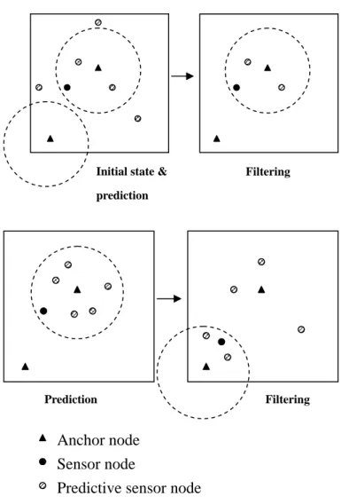
The key idea of MCL is to represent the posterior distribution of possible locations using a set of weighted samples. Each step is divided into a prediction phase and filtering phase. In the prediction phase, the sensor node makes a movement and the uncertainty of its position increases. In the filtering phase, new measurements (such as observations of new landmarks) are incorporated to filter and update data. The process repeats and the sensor node continually updates its predicted location [2].

In Figure 1, initially, a sensor node unknown of its location generates five samples in the prediction phase. Then, some anchor nodes observe two samples and filter out three impossible samples. In order to maintain five samples, this sensor node must resample three predictive sensor nodes. Finally, the other anchor nodes observe two samples and filter out three impossible samples. Over and over again, a sensor node can compute its location by these samples.

Figure 1. The process of the MCL algorithm.

2.2 CDL [1]

The CDL algorithm is a centralized localization algorithm that is based on the color theory to perform positioning in mobile WSNs. It builds a location database in the server, which maps a set of RGB values to a geographic position. And the distance measurements by sensor nodes are based on the DV-Hop [12]. When a sensor node receives anchors’ RGB values, it calculates its own RGB values. The node then sends its RGB values to the server so that the server can find the most possible location by looking up in the location database.

Prediction Filtering

Anchor node Sensor node

Predictive sensor node

Initial state & prediction

2.2.1 The Information Delivery of Anchors [1]

In this section, we introduce some notations that are defined in CDL:

¾ Each sensor i maintains an entry of (R_ik,G_ik,B_ik) and D , where k _ik

represents the kth anchor.

¾ D_avg is the average hop distance, which is based on DV-Hop [12]. ¾ h is the hop counts between sensors i and j. _ij

¾ D represents the hop distance from anchor k to node i; _ik D_ik =D_avg×h_ik

¾ Range represents the maximum distance that a color (brightness) can be propagated.

¾ (R_k,G_k,B_k) is the RGB value of anchor k.

¾ (Hik,Sik,Vik) is the HSV value of anchor k received by the i

th

sensor.

The RGB values of anchors are assigned randomly from 0 to 1. After a sensor i

obtains each anchor’s RGB value and hop count (h ), the RGB value is first _ik

converted to the HSV value by equation (1) [15]: )

, ,

(H_k S_k V_k = RGBtoHSV(R_k,G_k,B_k) (1) With h , ik D can be computed. The updated HSV value corresponding to ik

sensor i of anchor k is calculated by equation (2):

k ik H H = , Sik =Sk, k ik ik V Range D V =(1− )× (2)

The RGB value of sensor i corresponding to anchor k is then calculated: )

, ,

(R_ik G_ik B_ik = HSVtoRGB (H_ik,S_ik,V_ik) (3) The RGB value of sensor i is the mean of the RGB values corresponding to all

∑

where n is the number of anchors that sensor i received their RGB values.

2.2.2 The Establishment of Location Database [1]

A location database is established when the server obtains the RGB values and location of all anchors. The mechanism is based on the theorem of the mixture of different colors. With the RGB values of all anchors, the RGB values of all locations can be computed by exploiting the ideas of color propagation and the mixture of different colors. In the first place, the distance between each location i and anchor k is obtained:

ik d =

(

)

)

(

x

y

y

x

−

+

−

anchor k. First of all, we have to calculate the HSV value of each location i corresponding to anchor k: ) , , (H_k S_k V_k = RGBtoHSV(R_k,G_k,B_k) (6) k ik H H = , Sik =Sk , k ik ik V Range d V =(1− )• (7) The RGB value of location i corresponding to anchor k can be derived by equation (8):

) , ,

(R_ik G_ik B_ik = HSVtoRGB(H_ik,S_ik,V_ik) (8) Then the RGB value of location i can be calculated by averaging all RGB values of location i corresponding to N anchors.

∑

location database by maintaining the coordinate(x_i,y_i) and the RGB value )

, ,

(Ri Gi Bi at each location i. Then the location of a sensor node can be acquired

by looking up the location database based on the derived RGB value.

2.2.3 Mobility [1]

When a mobile node arrives at a new location, it sends an anchor information request to neighbor nodes. If the neighbor nodes have the anchors’ RGB values, they transmit packets that include the RGB value of each anchor and the hop count from the anchor to the node. After receiving the packets from neighbors, node i compares and calculates the D to the k_ik th anchor and get the smallestD . _ik

With the RGB values and D to all anchors, node i can update its RGB values ik

using equation (1), (2), (3), and (4). The new RGB values are then transmitted to the server and the position of node i will be updated by looking up the location database.

2.3 Comparison of Different Localization

Approaches

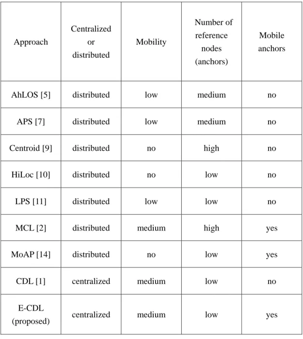
Some existing localization approaches are compared in Table 1. We take the following metrics into account: centralized or distributed, mobility, number of

reference nodes, and mobile anchors. The proposed E-CDL, which will be

described in Chapter 4, is also included in this table. The metric of centralized or distributed indicates it there is a central server taking responsibility for localization. Mobility indicates nodes in the network system are mobile or not. Number of reference nodes indicates the number of reference points required in each approach. Mobile anchors indicate that if the landmarks are mobile or not.

Approach Centralized or distributed Mobility Number of reference nodes (anchors) Mobile anchors

AhLOS [5] distributed low medium no

APS [7] distributed low medium no

Centroid [9] distributed no high no

HiLoc [10] distributed no low no

LPS [11] distributed low low no

MCL [2] distributed medium high yes

MoAP [14] distributed no low yes

CDL [1] centralized medium low no

E-CDL

(proposed) centralized medium low yes

Chapter 3

Design Approach

In this chapter, we propose a novel method, called E-CDL, to enhance the location accuracy of the CDL algorithm. Since CDL is based on the DV-hop approach [12], correct estimation of the average hop distance is very critical to location accuracy. Besides, by employing mobile anchor nodes, we can decrease possible isolations of sensor nodes in the multihop environment [12]. We will discuss these enhancements as follows.

3.1 Average Hop Distance Estimation

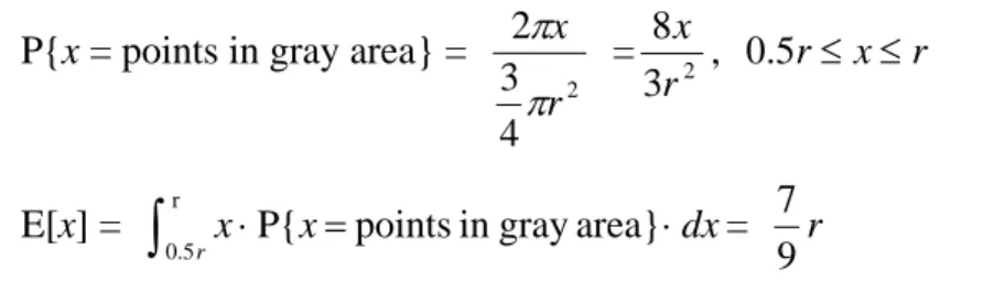
The first scheme is described below. We propose two simple and quick schemes to enhance the average hop distance estimate. When a sensor node intends to route data to some destination, it would select a nearby node that is close to the destination. According to this characteristic, we analyzed the behavior of sensors and discovered that they would select the next hop located between 0.5r and r (r is the radio range). As shown in Figure 2(a), sensor node S should choose a neighbor node 1 which is located larger than half of the radio range, as the next hop. However, in Figure 2(b), if sensor node S choose a neighbor nodes 1, which is located less than half of the radio range, as its next hop, the following hop (node 2) must be larger than half of the radio range; otherwise it will result in the situation of Figure 2 (c), where node 1 and 2 both are within the radio range. So it is expected that the candidate of the next hop should be located within the

area. We compute the expected value of the next hop distance as follows:

P{x = points in gray area} =

2 4 3 2 r x π π = ₂ 3 8 r x , 0.5r≤x≤r E[x] =

∫

0.5rx P{x pointsin gray area} dx= ₉r

7

The advantage of this enhancement is that it is simple and quick for estimating the average hop distance. Unlike the DV-Hop scheme, it must wait until the convergence of the topology to obtain a better average hop distance estimate.

Figure 2. (a) Sensor node S chooses node 1, which is located within the gray area, as the next hop; (b) Sensor node S chooses node 1, which is located less than half of the radio range, as the next hop; (c) Sensor node S chooses nodes 1 and 2 as its next two hops.

(a) (b) (c) S 1 2 S S 1 1 2 2 r: radio range S: sensor node

1, 2: next two hops

r r

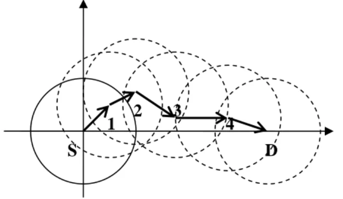
We now present our second scheme to further enhance the average hop distance estimate. In Figure 3, it is obvious that the shortest path length (S→1→2 →3→4→D) is larger than the Euclidean distance, SD, especially when the node density is low [16]. Apparently if the node density is large enough, the shortest path length will be close to the Euclidean distance. We have verified this observation via simulation. The average hop distance will be adjusted based on the ratio of the Euclidean distance to the shortest path length. We will derive such a ratio via simulation offline.

Figure 3. S→1→2→3→4→D is the shortest path from S to D. The straight line, SD, is apparently shorter than the shortest path.

S D

3.2 Mobility

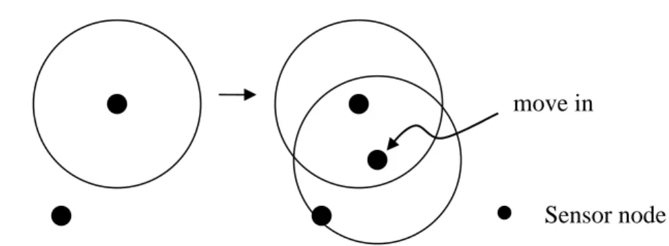
In order to further improve the location accuracy, we let anchor nodes as well as regular sensor nodes mobile in order to reduce possible isolations of sensor nodes in the multihop environment. As shown in Figure 4, sensor node movements can help reduce possible isolations of sensor nodes in the multihop environment. We put anchor nodes in the four corners of the square. And anchor nodes will move a radio range (r) along the square in every time slot. Some sensors may decrease their hop counts to anchor nodes, but other may increase. By employing mobile anchor nodes, we can reduce possible disconnections and the isolation problem of sensor nodes can be relieved. Therefore, the location accuracy can be improved. Finally, we summarize the E-CDL algorithm in Figure 5.

Figure 4. Sensor node movements can help reduce possible disconnections in the multihop environment.

move in

Start

1. Anchor nodes move a radio range r.

2. Anchor nodes deliver their RGB values and coordinates information to the sensor nodes and server

Location database is constructed by the server using Eq. (5), (6), (7), (8) and (9)

Each node obtains an average hop distance to each anchor node by (7r/9)×R

Sensor nodes update RGB values using Eq. (1), (2), (3) and (4)

Sensor nodes transmit the updated RGB values to the server

The server receives the RGB values from sensor nodes

The server calculates the coordinate of each sensor node by looking up the location database

Compute the ratio (R) of the Euclidean distance to the shortest path length offline.

To the server To sensor nodes

Chapter 4

Simulation Results and Discussions

In this chapter, we evaluate the proposed E-CDL algorithm. Besides, we have also implemented CDL [1] and MCL [2] for comparison.

4.1 Simulation Model

Our simulation model is a mobile WSN where all nodes are put in a 500 m × 500 m area and anchor nodes are placed in four corners. The simulation parameters are defined as follows:

z Sensor maximum speed (vmax): The maximum speed of sensor nodes.

z Sensor minimum speed (vmin): The minimum speed of sensor nodes.

z Anchor density (A ): The average number of anchor nodes in the radio _d

range.

z Sensor density (s ): The average number of sensor nodes in the radio range. _d

z Radio range (r): The radio transmission range.

z Ratio (R): The ratio of the Euclidean distance to the shortest path length. z CDL1: An enhanced CDL that sets the average hop distance to 7r/9. z CDL2: An enhanced CDL that adjusts the average hop distance by R. z CDL3: An enhanced CDL with mobile anchor nodes.

z E-CDL: CDL with the three enhancements.

We adopted the modified random waypoint model [2], in which nodes randomly choose their speed during each movement instead of choosing a speed for each destination. With this model, the average speed can be maintained at

addition, we assume the radio range is a perfect circle [2] and sensor nodes are uniformly distributed in the area. The simulation parameters are shown in Table 2. In addition, we compute the location error(ε)by,

(

) (

)

where

(

)

(

)

Parameter Value

Area size 500×500 m 2

Node speed Randomly choose from [Vmin,Vmax].

Radio range (r) 50 m

Pause time 0

Number of samples maintained

(MCL) 50

Measurement period 50 t_u

Time slot length (time unit) t_u

Anchor speed (E-CDL) r t_u

Table 2. Simulation parameters [2].

4.2 Simulation Results

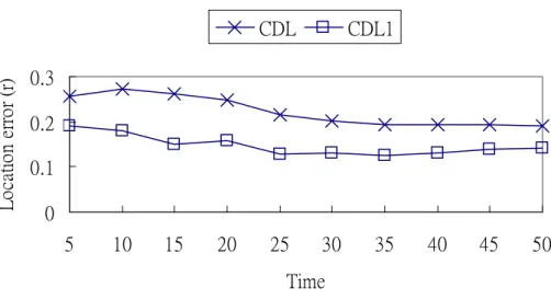
Based on Figure 2, our first enhancement is to set the average hop distance to 7r/9. In Figure 6, the location error has been reduced from 0.22r (CDL) to 0.15r (CDL1) in average.

0 0.1 0.2 0.3 5 10 15 20 25 30 35 40 45 50 Time L ocat io n er ro r (r ) CDL CDL1

Figure 6. Location errors of CDL1 via simulations. (s_d =10,v_max =r).

Our second enhancement is to compute the ratio of the Euclidean distance to the shortest path length (called hop distance adjusting ratio) offline for different source and destination pairs. Based on the sensor density (sd= 10), we randomly

generated different distribution of sensor nodes and compute the ratio(R) which is about 0.9. We used this ratio to adjust the average hop distance. In Figure 7, the location error has been reduced form 0.22r (CDL) to 0.13r (CDL2) in average.

0 0.1 0.2 0.3 5 10 15 20 25 30 35 40 45 50 Time L ocat io n er ro r (r ) CDL CDL2

Figure 7. Location errors of CDL2 via simulations. (s_d =10,v_max =r).

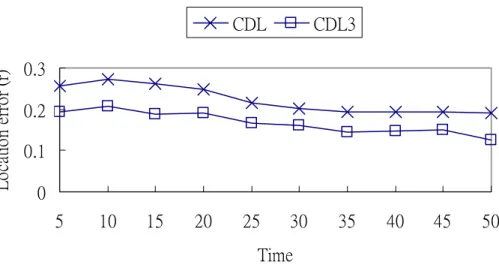
The last enhancement is to employ mobile anchor nodes. By allowing four mobile anchor nodes to move around the corners, the location error can be

reduced from 0.22r (CDL) to 0.17r (CDL2) in average. 0 0.1 0.2 0.3 5 10 15 20 25 30 35 40 45 50 Time L ocat io n er ro r (r ) CDL CDL3

Figure 8. Location errors of CDL3 via simulations. (s_d =10,v_max =r).

Finally, compare E-CDL, CDL, and MCL. These three range-free localization approaches are designed for mobile WSNs. Note that E-CDL is a CDL with the three enhancements. Figure 9 shows that location error of E-CDL (0.1r) is better than CDL (0.22r) and MCL (0.44r). Because MCL would exploit past information, its location error improves over time [2], and E-CDL and CDL perform stable over time [1].

0 0.5 1 1.5 2 5 10 15 20 25 30 35 40 45 50 Time L ocat io n er ro r (r ) CDL E-CDL MCL

Figure 9. Location accuracy comparison via simulations. s_d =10,v_max =r

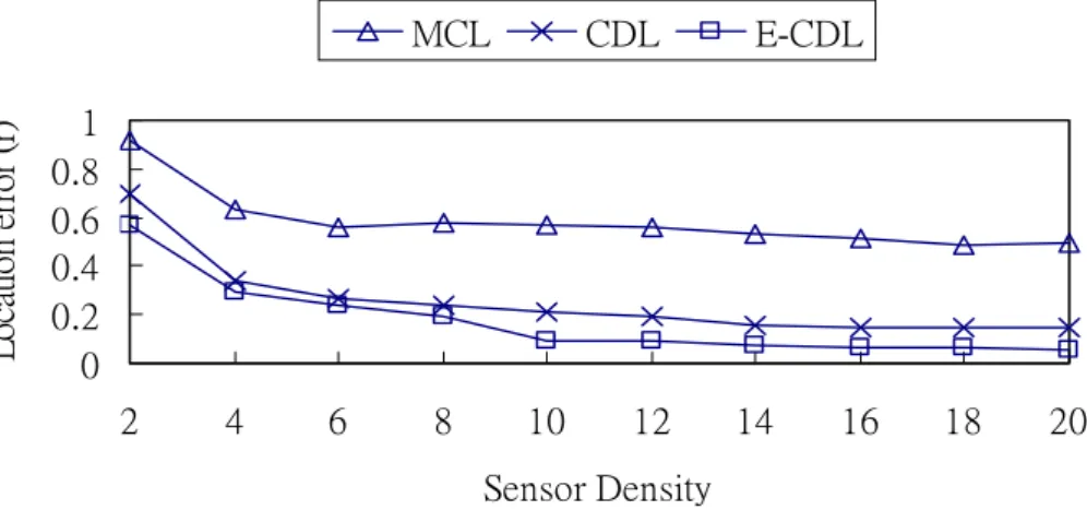
But if the sensor density is low, sensor nodes might not be uniformly distributed in the local area and the average hop distance would be inaccurate. Hence, when the sensor density is below 8, the location accuracy of E-CDL is close to CDL.

0 0.2 0.4 0.6 0.8 1 2 4 6 8 10 12 14 16 18 20 Sensor Density L o cat io n er ro r (r ) MCL CDL E-CDL

Figure 10. Impact of sensor density on location errors via simulations. (v_max =r).

We also evaluated the impact of anchor density on the location error of E-CDL. From simulation results, the location error of E-CDL with four anchor nodes in the corners is about 0.1r. If we place more anchor nodes (A_d =0.5), the location error stays within 0.09r. Therefore, we only placed four anchor nodes in the corners for localization.

Chapter 5

Experiments

5.1 Experimental Setup

We have implemented and evaluated E-CDL on the MICAz Mote Development Kit [3]. The MICAz is a 2.4GHz, Zigbee compliant Mote module used for enabling low-power, wireless sensor networks [3]. The MICAz uses the nesC language [17] on the TinyOS platform. It can be used for residential or building monitoring and security, and hospital health-care systems. We can easily construct a localization system with this kit. We conducted several experiments in a 20 m × 20 m area with seven motes. And, we chose three motes as anchor nodes and four as sensor nodes. Sensor nodes were randomly deployed in the area; however, there are two ways to deploy anchor nodes: (1) anchor nodes deployed randomly and (2) anchor nodes deployed in the corners. We will compare these two schemes in section 5.2.

5.2 Experimental Results

5.2.1 Anchor nodes deployed randomly

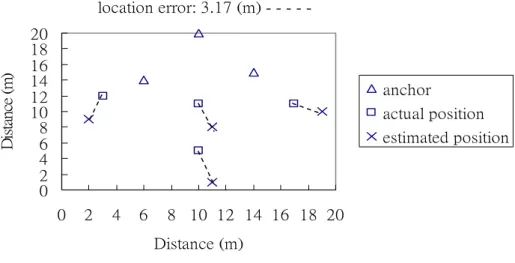
In this experiment, we first implemented the CDL algorithm with sensor and anchor nodes randomly deployed. In Figure 11, the location error of CDL is about 4.76 m. To enhance the localization accuracy, we computed the hop distance adjusting ratio (R) offline for different distribution of source and destination pairs.

In Figure 12, the location error of CDL2 is about 3.17 m which is better than that of CDL (4.76 m). location error: 4.76 (m) -0 2 4 6 8 10 12 14 16 18 20 0 2 4 6 8 10 12 14 16 18 20 Distance (m) Di st an ce ( m ) anchor actual position estimated position

Figure 11. Location errors of CDL via experiments with random anchors.

location error: 3.17 (m) -0 2 4 6 8 10 12 14 16 18 20 0 2 4 6 8 10 12 14 16 18 20 Distance (m) Di st an ce ( m) _anchor actual position estimated position

Figure 12. Location errors of CDL2 via experiments with random anchors.

5.2.2 Anchor nodes deployed in the corners

adjust the average hop distance. In Figure 14, the location error of CDL2 is about 1.87 m. This demonstrated that the location error of CDL has been reduced from 4.76 m to 2.38 m and that of CDL2 has been reduced from 3.17 m to 1.87 m by placing the anchor nodes in the corners. Therefore putting anchor nodes in the corners can improve the location accuracy.

location error: 2.38 (m) ---0 2 4 6 8 10 12 14 16 18 20 22 0 2 4 6 8 10 12 14 16 18 Distance (m) Di st an ce ( m ) anchor actual position estimated position

Figure 13. Location errors of CDL via experiments with anchor in the corners.

location error: 1.87 (m) ---0 2 4 6 8 10 12 14 16 18 20 22 0 2 4 6 8 10 12 14 16 18 Distance (m) Di st an ce ( m ) anchor actual position estimated position

5.3 Comparison of Simulation and Experiment

Results

In Chapter 4, the location errors of E-CDL from simulation results are about 0.1r, which is apparently better than the location error (0.21r) from experimental results. This is because the sample size for experiments was small and sensor nodes were stationary. In this situation, sensor nodes might not be uniformly distributed and might result in possible disconnections. In the future work, we will use a large sample size and mobile sensors to further validate the location accuracy of E-CDL.

Chapter 6

Conclusions and Future Work

6.1 Concluding Remarks

Localization is a critical issue in mobile WSNs. With the aid of location information of sensor nodes, for instance, the efficiency of routing can be improved. In this thesis, we have presented an E-CDL algorithm which is an enhanced color-theory-based dynamic localization algorithm, which uses three enhancements to improve the location accuracy of the original CDL algorithm. The basic idea of the enhancements is more accurate estimate of the average hop distance and with the assistance of mobile anchor nodes that are placed in the corners. Simulation results have shown that the location error is about 0.1r when the sensor density is 10 and the maximum speed is r t_u . However, the experimental results show that the location error is only 0.21r. This is due to a limited sample size. In addition, the location accuracy of E-CDL is 50% - 55% better than that of CDL, and 75% - 80% better than that of MCL. In summary, E-CDL is an efficient range-free and centralized localization scheme and is therefore very suitable for health-care and hospital monitoring systems.

6.2 Future Work

We have proposed three enhancements to further enhance the original CDL algorithm. However, routing is not considered in the thesis. Therefore, we are going to combine our localization method with a routing algorithm to propose an efficient location-aware routing algorithm. In addition, in the experiments,

might not be uniformly distributed and might result in the possible isolations of sensor nodes. We will use a larger sample size and mobile nodes to further validate the location accuracy of E-CDL. Finally, we will implement our algorithm combing with a routing algorithm in a heath-care system to further evaluate the effectiveness of E-CDL in real systems.

Bibliography

[1] S.-H. Shee, K.-C. Wang and I.-L. Hsieh “Color-theory-based Dynamic Localization in Mobile Wireless Sensor Networks,” in Proceedings of

Workshop on Wireless Ad Hoc Sensor Networks, Aug 2005.

[2] H. Lingxuan and E. David, “Localization for Mobile Sensor Networks,” in

Proceedings of International Conference on Mobile Computing and Networking, Sept 2004, pp. 45–57.

[3] Crossbow Technology, Inc. http://www.xbow.com/.

[4] D. Niculescu, “Positioning in Ad Hoc Sensor Networks,” IEEE Network, July-Aug. 2004, pp. 24–29.

[5] A. Savvides, C.-C. Han, and M. Srivastava, “Dynamic Fine-grained Localization in Ad-hoc Networks of Sensors,” in Proceedings of ACM

MOBICOM, 2001, pp. 166–179.

[6] A. Savvides, H. Park, and M. Srivastava, “The n-Hop Multilateration Primitive for Node Localization Problems,” Mobile Networks and

Applications, Volume 8, Issue 4, 2003, pp. 443–451.

[7] D. Niculescu and B. Nath, “Position and Orientation in Ad Hoc Networks,”

Elsevier Ad Hoc Networks, vol. 2, no. 2, Apr. 2004, pp. 133–51.

[8] D. Niculescu and B. Nath, “Ad Hoc Positioning System(APS), ” In

Proceeding of IEEE GLOBECOM’01, Volume 5 , Nov 2001, pp. 2926–2931. [9] N. Bulusu, J. Heidemann and D. Estrin, “GPS-less Low Cost Outdoor

[10] L. Lazos and R. Poovendran, “HiRLoc: High-resolution Robust Localization for Wireless Sensor Networks,” IEEE Journal on Selected Areas in

Communications, Volume 24, Issue 2, Feb. 2006, pp. 233–246.

[11] D.Niculescu and B. Nath, “Localized Positioning in Ad Hoc Networks,”

Elsevier Ad Hoc Networks, vol. 1, no. 2–3, Sept. 2003, pp. 247–59.

[12] J.-G. Lim and S.-V. Rao, “Mobility-enhanced Positioning in Ad Hoc Networks”, WCNC 2003, vol.3, Mar. 2003, pp. 1832–1837.

[13] R.-K. Patro,” Localization in Wireless Sensor Network with Mobile Beacons,” in Proceedings of 23rd IEEE Convention of Electrical and

Electronics Engineers, Sept. 2004, pp. 22–24.

[14] K.-F. Ssu, C.-H. Ou and H.-C. Jiau, “Localization with Mobile Anchor Points in Wireless Sensor Networks,” IEEE Transactions on Vehicular Technology, May 2005, pp. 1187–1197.

[15] E. Vishnevsky, “RGB to HSV & HSV to RGB” [Online] Available: http://www.cs.rit.edu/~ncs/color/t_convert.html

[16] H. Wu, C. Wang and N.-F. Tzeng, “Novel Self-configurable Positioning Technique for Multihop Wireless Networks,” IEEE/ACM Transactions on

Networking (TON), v.13, no.3, pp. 609–621, June 2005.

[17] D. Gay, P. Levis and R. Behren, “The nesC Language: A Holistic Approach to Networked Embedded Systems,” in Proceedings of Programming