類別資料在兩個經驗貝氏模型中的模型選取技術

全文

(1)國立交通大學統計學研究所碩士論文. 類別資料在兩個經驗貝氏模型中的模型選取技術 A Model Selection Technique between Two Empirical Bayes Models for Categorical Data. 研究生：劉振熒指導教授：陳志榮. 教授. 中華民國九十四年六月.

(2) 類別資料在兩個經驗貝氏模型中的模型選取技術 A Model Selection Technique between Two Empirical Bayes Models for Categorical Data. 研究生：劉振熒. Student：Chen-Ying Liu. 指導教授：陳志榮博士. Advisor：Dr. Chih-Rung Chen. 國立交通大學統計學研究所碩士論文. A Thesis Submitted to Department of Computer and Information Science College of Electrical Engineering and Computer Science National Chiao Tung University in partial Fulfillment of the Requirements for the Degree of Master in. Statistics June 2005 Hsinchu, Taiwan, Republic of China. 中華民國九十四年六月.

(3) 類別資料在兩個經驗貝氏模型中的模型選取技術. 指導教授：陳志榮. 學生：劉振熒. 教授. 國立交通大學統計學研究所碩士班. 摘. 要. 在本篇論文中，首先我們提出一個對於製程中的類別資料在兩個經驗貝氏模型中的模型選取技術。然後我們簡介可用於製程中類別資料的兩個有用的經驗貝氏模型。最後舉一個例子並透過模擬實驗來展示所提出的方法之表現。. 關鍵字: 經驗貝氏; 製程監控; 類別資料; beta-二項式; Dirichlet-多項式; 變換-常態-二項式; 變換-常態-多項式; 管制圖; 品質管制.. i.

(4) A Model Selection Technique between Two Empirical Bayes Models for Categorical Data student：Chen-Ying Liu. Advisors：Dr. Chih-Rung Chen. Institute of Statistics National Chiao Tung University. ABSTRACT. In the paper, first of all, a model selection technique between two empirical Bayes models for categorical data in manufacturing is proposed. Next, two useful empirical Bayes models for categorical data in manufacturing are introduced. Finally, the performance of the proposed method is illustrated by an example through simulations.. KEY WORDS: Empirical Bayes; Process monitoring; Categorical data; Beta-binomial; Dirichlet-multinomial; Transformed-normal-binomial; Transformed-normal-multinomial; Control chart; Quality control.. ii.

(5) 誌. 謝. 光陰荏苒，轉眼已至鳳凰花開和驪歌清唱時分，興奮愉悅與悵然不捨的情緒參雜交錯，心中感慨萬千。回首統研所兩年歲月的風風雨雨，品嚐到生命的酸甜苦辣，仍記憶猶新，歷歷在目。研究室的熱烈討論聲跟球場上揮灑的汗水，隨著時間緣起緣滅，終究要劃下一個美麗的句點。首先，所上每位老師孜孜不倦的教導，如沐春風，除了富含高深的專業學問和不懈的研究精神外，其待人接物跟處事哲學，皆惠我良多且開闊了寬廣的視野，誠可作為學習的榜樣。特別要由衷感激指導教授陳志榮老師，不但教學認真與治學嚴謹，更熱心地為學生解惑。感謝這一年多來不遺餘力的悉心教誨和指點，鉅細靡遺地傾囊相授，不厭其煩地耐心幫忙審稿校正，實在是令人敬佩不已。師恩浩瀚，永銘於心。同時，承蒙洪慧念老師、黃榮臣老師以及許文郁老師能撥冗抽空來蒞臨指教，並提供許多寶貴的建議，使論文更臻完美。其次，感謝助理們於行政事務跟電腦方面的支援，使其能順利畢業。對於已畢業的小慧與姿吟學姊所提供的協助及經驗分享，銘感五內，而學長姐、同學、朋友跟學弟妹們的陪伴與關心，互相切磋和砥礪，培養出彌足珍貴的友誼，在艱辛的生活中備感溫暖且不顯孤單。另外，還需感謝家人們的照顧與栽培，尤其是含辛茹苦的母親，多年來無怨無悔的付出，在我學習低潮、碰到瓶頸或挫敗氣餒時，適時給予了精神上的關懷跟鼓勵，化作堅實的後盾，令我提起勇氣堅強面對諸多挑戰，得以心無旁鶩地焚膏繼晷、披荊斬棘，潛心於研究，以致完成論文。也因為有您，才能造就今日的我。最後，感謝交大優良的求學環境、師長父母的教養恩澤及同窗好友的勉勵扶持，不過心中的謝意難以用隻字片語表達，只好奉上最誠摯的祝福，願各位順心如意，謹將此拙著獻給大家，一同分享這份成就和喜悅。此刻，即將揮別研究所的生涯，懷抱著美好的回憶繼續邁入人生的另一段旅程，雖說天下無不散的筵席，但冀望未來的路途能有緣與你們相聚。. 劉振熒謹誌于國立交通大學統計學研究所中華民國九十四年六月. iii.

(6) 目. 錄. Abstract in Chinese ..................................................................................... i Abstract in English..................................................................................... ii Acknowledgement .................................................................................... iii Contents .................................................................................................... iv 1. Introduction......................................................................................... 1 2. A model selection technique............................................................... 4 3. An example ....................................................................................... 12 4. A simulation study ............................................................................ 15 5. Conclusions and future work ............................................................ 24 Appendix.................................................................................................. 25 References................................................................................................ 26. iv.

(7) 1. INTRODUCTION. In a manufacturing process, suppose that there are k possible types of defects in a product for some known positive integer k. For each tested product item, the result could be classified as one and only one of the following k + 1 disjoint categories: {the first defect type, . . ., the kth defect type, pass}. Such data are called either binary for k = 1 or polytomous for k ≥ 2. In the paper, categorical data denote either binary data for k = 1 or polytomous data for k ≥ 2. See, e.g., McCullagh and Nelder (1989, Chapters 4 and 5) or Agresti (2002) for the categorical data analysis. In the Bayesian framework, it is assumed that the unknown random parameters have a known prior distribution. In practice, choosing an appropriate subjective or objective prior distribution is usually a non-trivial task for practitioners. Instead of a Bayesian approach, an empirical Bayes approach is commonly used in the literature. For an empirical Bayes inference, the marginal distribution of the observed data is utilized to estimate the unknown hyperparameters and then a Bayesian inference is made for the random parameters as if the estimated prior distribution were the prior distribution. There are some researches for the empirical Bayes process monitoring techniques for categorical data in manufacturing. For example, Yousry et al. (1991) used the beta-binomial empirical Bayes model for binary data utilizing the method of moments for estimation of the hyperparameters. Recently, Shiau et al. (2005) used the Dirichlet-multinomial empirical Bayes model for polytomous data utilizing both the method of moments and the pseudo-. 1.

(8) likelihood method for estimation of the hyperparameters. Chen et al. (2004) used the betabinomial or Dirichlet-multinomial empirical Bayes model for categorical data utilizing the maximum likelihood (ML) method for estimation of the hyperparameters and the likelihood ratio (LR) method for monitoring the manufacturing process. Similarly, Chen et al. (2005) used the transformed-normal-binomial or transformed-normal-multinomial empirical Bayes model for categorical data utilizing the same methods as Chen et al. (2004). To proceed the discussion, we first briefly introduce a Bayesian inference as follows: In the Bayesian framework, it is assumed that the unknown random parameter vector θ has a known prior probability density function (p.d.f.) or probability mass function (p.m.f.) π(θ) and that the response vector y has a known conditional p.d.f. or p.m.f. f (y|θ) given θ. Then a Bayesian inference is based on the posterior p.d.f. or p.m.f., p(θ|y), of θ given y, where. p(θ|y) ∝ f (y|θ) π(θ).. It is common practice to estimate θ by the posterior mean, E(θ|y), or the posterior mode, mode(θ|y), of θ given y, where R P θ f (y|θ) π(θ) dθ θ f (y|θ) π(θ) Θ or Pθ∈Θ E(θ|y) = R θ∈Θ f (y|θ) π(θ) Θ f (y|θ) π(θ) dθ and mode(θ|y) = arg sup p(θ|y) = arg sup f (y|θ) π(θ) θ∈Θ. θ∈Θ. with P ({θ ∈ Θ}) = 1. See, e.g., Gelman et al. (2004) or O’Hagan and Forster (2004) for the Bayesian data analysis.. 2.

(9) Next, we briefly introduce an empirical Bayes inference as follows: In the empirical Bayes framework, it is assumed that the unknown random parameter vector θ has a prior p.d.f. or p.m.f. π(θ; λ) and that the response vector y has a known conditional p.d.f. or p.m.f. f (y|θ) given θ, where λ is an unknown hyperparameter vector and π(·; ·) is a known function. Then an empirical Bayes inference is based on the estimated posterior p.d.f. or p.m.f., p(θ|y; λ)|λ=λ(y) , of θ given y, where ˆ p(θ|y; λ) ∝ f (y|θ) π(θ; λ) ˆ ˆ and λ(y) is an estimator of λ. In practice, λ(y) is frequently chosen as the maximum likelihood estimator (MLE) or a method-of-moments estimator (MME) of λ. Similarly, it is common practice to estimate θ by the estimated posterior mean, E(θ|y; λ)|λ=λ(y) , or the ˆ estimated posterior mode, mode(θ|y; λ)|λ=λ(y) , of θ given y, where ˆ R P θ f (y|θ) π(θ; λ) dθ θ f (y|θ) π(θ; λ) Θ or Pθ∈Θ E(θ|y; λ) = R θ∈Θ f (y|θ) π(θ; λ) Θ f (y|θ) π(θ; λ) dθ and mode(θ|y; λ) = arg sup p(θ|y; λ) = arg sup f (y|θ) π(θ; λ) θ∈Θ. θ∈Θ. with P ({θ ∈ Θ}; λ) = 1. See, e.g., Carlin and Louis (2000) for the empirical Bayes data analysis. The remaining part of the paper is organized as follows. A model selection technique between two empirical Bayes models for categorical data in manufacturing is proposed in Section 2. In Section 3, two useful empirical Bayes models for categorical data are. 3.

(10) introduced. The performance of the proposed method is illustrated by an example through simulations in Section 4. Some concluding remarks and future work are given in Section 5.. 2. A MODEL SELECTION TECHNIQUE. Assume that each tested product item is classified as one and only one of the following k + 1 categories: {the first defect type, . . ., the kth defect type, pass}, where k is a known positive integer. Let t be any positive integer. Suppose that there are nt tested product items manufactured at time t, where nt is a known positive integer. For i ∈ {1, . . . , k}, let θit denote the probability that a product item manufactured at time t is of the ith defect type. Then 1 −. Pk. i=1 θit. (≡ θk+1,t ) is the probability that a product item manufactured at. time t passes the test. Assume that θit > 0 for i ∈ {1, . . . , k + 1}. For i ∈ {1, . . . , k}, let yit denote the number of the tested product items which are of the ith defect type among the nt tested product items manufactured at time t. Then nt −. Pk. i=1 yit. (≡ yk+1,t ) is the. number of the tested product items which pass the test among the nt tested product items manufactured at time t. Set θt ≡ (θ1t , . . . , θkt )T , yt ≡ (y1t , . . . , ykt )T , Θ ≡ {θt : θ1t , . . . , θkt > 0 and. Pk. i=1 θit. < 1}, and Ynt ≡ {yt : y1t , . . . , ykt ∈ {0, 1, . . . , nt } and. Pk. i=1 yit. ≤ nt }.. Assume that yt has the conditional binomial(nt ; θt ) or multinomial(nt ; θt ) distribution given θt . Let Fθt and Fyt |θt denote, respectively, the prior cumulative distribution function (c.d.f.) of θt and the conditional c.d.f. of yt given θt . Then yt has the conditional p.m.f. nt !. f (yt |θt ) = 1Ynt (yt ) · Qk+1 i=1. 4. yit !. ·. k+1 Y i=1. yit θit. (1).

(11) given θt , where 1Ynt (yt ) = 1 for yt ∈ Ynt and 0 otherwise. Thus, yt has the marginal p.m.f. nt ! f (yt ; Fθt ) = 1Ynt (yt ) · Qk+1 i=1. yit !. ·. Z k+1 Y Θ i=1. yit θit dFθt (θt ).. (2). Throughout the paper, we say that the manufacturing process is in control at time t when Fθt = F , where F is a c.d.f. on Θ with some unknown p.d.f. π(·). For any positive integer m, set Rm ≡ (−∞, ∞)m , let 0m×1 denote the m × 1 vector (0, . . . , 0)T , and let 1m×1 denote the m × 1 vector (1, . . . , 1)T . For u ∈ {1, 2}, let model u denote the parametric family {Fu,λu : λu ∈ Λu }, where λu is a qu ×1 hyperparameter vector for some known positive integer qu , each Fu,λu is a c.d.f. on Θ with known p.d.f. πu (·; λu ), and Λu is a known open subset of Rqu . Without loss of generality, assume that q1 ≤ q2 . Assume that ∂ 2 πu (θt ; λu )/∂λu ∂λTu exists for θt ∈ Θ, λu ∈ Λu , and u ∈ {1, 2}. For λu ∈ Λu and u ∈ {1, 2}, let Fyt ;u,λu denote the marginal c.d.f. of yt when Fθt = Fu,λu . Then yt has the marginal p.m.f. nt ! f (yt ; Fu,λu ) = 1Ynt (yt ) · Qk+1 i=1. yit !. ·. Z k+1 Y Θ i=1. yit θit dFu,λu (θt ). (3). when Fθt = Fu,λu for some λu ∈ Λu and u ∈ {1, 2}. For λu ∈ Λu and u ∈ {1, 2}, the Kullback-Leibler distance between F and Fu,λu is ·. Z d (F, Fu,λu ) ≡. log Θ. ¸ π(θt ) dF (θt ) (≡ du (λu )). πu (θt ; λu ). By the Jensen inequality, ¸ ¸ ·Z πu (θt ; λu ) πu (θt ; λu ) · π(θt ) dθt dF (θt ) ≥ − log du (λu ) = − log π(θt ) π(θt ) Θ Θ "Z # ¸ ·Z = − log πu (θt ; λu ) dθt = 0, πu (θt ; λu ) dθt ≥ − log. Z. ·. Θ. {θt :π(θt )>0}. 5. (4).

(12) where du (λu ) = 0 if and only if Fu,λu = F . For λu ∈ Λu and u ∈ {1, 2}, assume that all of the following conditions hold: du (λu ) < ∞, ∂ 2 du (λu )/∂λu ∂λTu exists, Z. ∂du (λu ) = ∂λu. Θ. ∂ ∂λu. ½ · log. π(θt ) πu (θt ; λu ). ¸¾ dF (θt ),. and ∂ 2 du (λu ) = ∂λu ∂λTu. Z Θ. ∂2 ∂λu ∂λTu. ½ · log. π(θt ) πu (θt ; λu ). ¸¾ dF (θt ).. For u ∈ {1, 2}, assume that there exists a unique λ0u ∈ Λu such that λ0u = arg inf du (λu ). λu ∈Λu. (5). Suppose that we are interested in choosing either model 1 or model 2 as an approximate model for monitoring the manufacturing process. For this purpose, we would like to consider the hypothesis testing problem with the null hypothesis H0 : d1 (λ01 ) ≤ d2 (λ02 ) versus the alternative H1 : d1 (λ01 ) > d2 (λ02 ). Then we choose model 2 if and only if we reject H0 in favor of H1 . Note that ∂du (λu )/∂λu |λu =λ0u = 0qu ×1 for u ∈ {1, 2}. For λu ∈ Λu and u ∈ {1, 2}, set gu (λu ) ≡ −∂du (λu )/∂λu and hu (λu ) ≡ −∂gu (λu )/∂λTu . Then, for λu ∈ Λu and u ∈ {1, 2}, Z gu (λu ) =. Θ. Z ≡. Θ. ∂πu (θt ; λu )/∂λu dF (θt ) πu (θt ; λu ) Su (λu ; θt ) dF (θt ) ≡ E (Su (λu ; θt ); F ). 6. (6).

(13) and Z hu (λu ) =. − Θ. Z ≡. Θ. ∂Su (λu ; θt ) dF (θt ) ∂λTu. Ju (λu ; θt ) dF (θt ) ≡ E (Ju (λu ; θt ); F ) .. (7). When both gu (λu ) and hu (λu ) have closed-form formulas for λu ∈ Λu and u ∈ {1, 2} in a simulation study, we may utilize the following Newton-Raphson method to obtain λ0u : First 0(0). choose a good initial value λu. for λ0u and then iterate the following equations. h ³ í−1 ³ ´ λ0(v+1) = λ0(v) + hu λ0(v) gu λ0(v) u u u u 0(v). for v = 0, 1, . . . until λu. (8). converges to λ0u . When gu (λu ) or hu (λu ) does not have a closed-. form formula for some λu ∈ Λu and u ∈ {1, 2} in a simulation study, we may first simulate (1). (R). an i.i.d. sample {θt , . . . , θt } of size R, e.g., R = 100 000, from the c.d.f. F and then numerically evaluate gu (λu ) and hu (λu ) by R−1 ·. PR. (r) r=1 Su (λu ; θt ). and R−1 ·. PR. (r) r=1 Ju (λu ; θt ),. respectively. Suppose that there is an available in-control historical data set {y1 , . . . , yT } in the manufacturing process for some known positive integer T , where (θ1T , y1T )T , . . . , (θTT , yTT )T are independent 2k × 1 random vectors. Set θ ≡ (θ1T , . . . , θTT )T , y ≡ (y1T , . . . , yTT )T , and Y ≡ Yn1 × · · · × YnT . Given y and under model u for u ∈ {1, 2}, the log-likelihood function for λu is. ù (λu ; y) ≡ log. "T Y t=1. # f (yt ; Fu,λu ). =. T X t=1. 7. log[f (yt ; Fu,λu )] ≡. T X t=1. ù (λu ; yt ),. (9).

(14) the score function for λu is. Su (λu ; y) ≡. ∂ù (λu ; y) ∂λu. =. T X ∂ù (λu ; yt ) t=1. T X ∂f (yt ; Fu,λu )/∂λu = f (yt ; Fu,λu ). ∂λu ≡. t=1. T X. Su (λu ; yt ),. (10). t=1. and the observed (Fisher) information for λu is. Ju (λu ; y) ≡ −. ∂Su (λu ; y) ∂λTu. =. T X. −. t=1. ∂Su (λu ; yt ) ∂λTu. ≡. T X. Ju (λu ; yt ).. (11). t=1. ˆ u (y) (≡ λ ˆ u ) of λu solves the Given y and under model u for u ∈ {1, 2}, the MLE λ ˆ u ) = 0q ×1 for u ∈ {1, 2}. We may score equation Su (λu ) = 0qu ×1 for λu . That is, Su (λ u ˆ u for u ∈ {1, 2}: First choose a utilize the following Newton-Raphson method to obtain λ ˆ (0) ˆ good initial value λ u for λu and then iterate the following equations ´ í−1 ³ h ³ ˆ (v) ; y ˆ (v) ; y ˆ (v+1) = λ ˆ (v) + Ju λ λ S λ u u u u u. (12). ˆ u(v) converges to λ û. for v = 0, 1, . . . until λ Let Fy denote the c.d.f. of y with p.m.f. f (y; F ). For λu ∈ Λu and u ∈ {1, 2}, let Fy;u,λu denote the c.d.f. of y with p.m.f. f (y; Fu,λu ) when Fθ1 = . . . = FθT = Fu,λu . For λu ∈ Λu and u ∈ {1, 2}, the Kullback-Leibler distance between Fy and Fy;u,λu is ¸ f (y; F ) f (y; F ) d (Fy , Fy;u,λu ) ≡ log f (y; Fu,λu ) y∈Y   ¸ · T  X  X f (yt ; F ) f (yt ; F ) = log   f (yt ; Fu,λu ). X. t=1. ≡. T X. ·. yt ∈Ynt. d (Fyt , Fyt ;u,λu ) (≡ dun1 ,...,nT (λu )).. t=1. 8. (13).

(15) For u ∈ {1, 2}, assume that there exists a unique λun1 ,...,nT ∈ Λu such that λun1 ,...,nT = arg inf dun1 ,...,nT (λu ).. (14). λu ∈Λu. When n1 = . . . = nT , set dnu1 (λu ) ≡ dun1 ,...,nT (λu ) and λnu1 ≡ λun1 ,...,nT for λu ∈ Λu and u ∈ {1, 2}. Then dnu1 (λu ) = T · d (Fy1 , Fy1 ;u,λu ) for λu ∈ Λu and u ∈ {1, 2}. Note that ∂dun1 ,...,nT (λu )/∂λu |λu =λnu1 ,...,nT = 0qu ×1 for u ∈ {1, 2}. For λu ∈ Λu and u ∈ {1, 2}, set gun1 ,...,nT (λu ) ≡ −T −1 ·∂dun1 ,...,nT (λu )/∂λu and hun1 ,...,nT (λu ) ≡ −T −1 ·∂gun1 ,...,nT (λu ) /∂λTu . Then, for λu ∈ Λu and u ∈ {1, 2},   ! Ã T T X X X 1 1 n1 ,...,nT  · Su (λu ; yt ); F Su (λu ; yt ) f (yt ; F ) = E gu (λu ) = · T T t=1. (15). t=1. yt ∈Ynt. and   ! Ã T T X X X 1 1  · Ju (λu ; yt ); F . Ju (λu ; yt ) f (yt ; F ) = E hun1 ,...,nT (λu ) = · T T t=1. (16). t=1. yt ∈Ynt. When n1 = . . . = nT , set gun1 (λu ) ≡ gun1 ,...,nT (λu ) and hnu1 (λu ) ≡ hun1 ,...,nT (λu ) for λu ∈ Λu and u ∈ {1, 2}. Then gun1 (λu ) =. X. Su (λu ; y1 ) f (y1 ; F ) = E (Su (λu ; y1 ); F ). (17). Ju (λu ; y1 ) f (y1 ; F ) = E (Ju (λu ; y1 ); F ). (18). y1 ∈Yn1. and hnu1 (λu ) =. X y1 ∈Yn1. ˆ u = λn1 + for λu ∈ Λu and u ∈ {1, 2}. When n1 = . . . = nT , it can be shown that λ u √ Op (1/ T ) as T → ∞ for λu ∈ Λu and u ∈ {1, 2}. Thus, it is very likely that λun1 ,...,nT ≈ ˆ u ≈ λ0 for large T and min{n1 , . . . , nT }. λ0u for large min{n1 , . . . , nT } and λ u 9.

(16) When both gun1 ,...,nT (λu ) and hun1 ,...,nT (λu ) have closed-form formulas for λu ∈ Λu and u ∈ {1, 2} in a simulation study, we may utilize the following Newton-Raphson method to n ,...,nT (0). obtain λun1 ,...,nT : First choose a good initial value λu1. for λun1 ,...,nT and then iterate. the following equations h ³ í−1 ³ ´ λun1 ,...,nT (v+1) = λun1 ,...,nT (v) + hun1 ,...,nT λun1 ,...,nT (v) gun1 ,...,nT λun1 ,...,nT (v) n ,...,nT (v). for v = 0, 1, . . . until λu1. (19). converges to λun1 ,...,nT . When gun1 ,...,nT (λu ) or hun1 ,...,nT (λu ). does not have a closed-form formula for some λu ∈ Λu and u ∈ {1, 2} in a simulation study, we may first simulate an i.i.d. sample {y(1) , . . . , y(R) } of size R, e.g., R = 100 000, from the c.d.f. Fy and then numerically evaluate gun1 ,...,nT (λu ) and hun1 ,...,nT (λu ) by R−1 · PT. (r) t=1 Su (λu ; yt )]. and R−1 ·. PR. r=1 [T. −1. ·. PT. (r) t=1 Ju (λu ; yt )],. PR. r=1 [T. −1. ·. respectively.. When n1 = . . . = nT and both gun1 (λu ) and hnu1 (λu ) have closed-form formulas for λu ∈ Λu and u ∈ {1, 2} in a simulation study, we may utilize the following Newton-Raphson n (0). method to obtain λnu1 : First choose a good initial value λu1. for λnu1 and then iterate the. following equations h ³ í−1 ³ ´ λun1 (v+1) = λun1 (v) + hnu1 λun1 (v) gun1 λun1 (v) n (v). for v = 0, 1, . . . until λu1. (20). converges to λnu1 . When gun1 (λu ) or hnu1 (λu ) does not have a. closed-form formula for some λu ∈ Λu and u ∈ {1, 2} in a simulation study, we may simply (1). (R). simulate an i.i.d. sample {y1 , . . . , y1 } of size R, e.g., R = 100 000, from the c.d.f. Fy1 and then numerically evaluate gun1 (λu ) and hnu1 (λu ) by R−1 · (r). Ju (λu ; y1 ), respectively. 10. PR. (r) r=1 Su (λu ; y1 ). and R−1 ·. PR. r=1.

(17) Now, consider the simple case where F belongs to either model 1 or model 2. For λ1 ∈ Λ1 , λ2 ∈ Λ2 , and y ∈ Y, set ½ φ∗λ1 ,λ2 (y). ≡. 1 for f (y; F1,λ1 ) < f (y; F2,λ2 ), 0 otherwise.. (21). Then φ∗λ1 ,λ2 |λ1 =λ01 ,λ2 =λ02 (≡ φ∗λ0 ,λ0 ) is the likelihood ratio test (LRT) for testing the new 1. 2. hypothesis testing problem with the null hypothesis H00 : F = F1,λ01 versus the alternative H10 : F = F2,λ02 . Let φ be any randomized test, i.e., 0 ≤ φ(y) ≤ 1 for y ∈ Y. When y is observed and the randomized test φ is used for this new hypothesis testing problem, we reject H00 in favor of H10 with probability φ(y). For any randomized test φ, let αφ and βφ denote, respectively, the type I error and the type II error of φ for this new hypothesis testing problem. Then, for any randomized test φ, X. αφ + βφ = = 1+. X y∈Y. ≥ 1+. X. y∈Y. y∈Y. ´ X ³ ´ ³ φ(y) f y; F1,λ01 + [1 − φ(y)] f y; F2,λ02 y∈Y. í ´ ³ h ³ φ(y) f y; F1,λ01 − f y; F2,λ02 í ´ ³ h ³ = αφ∗ 0 φ∗λ0 ,λ0 (y) f y; F1,λ01 − f y; F2,λ02 1. λ1 ,λ0 2. 2. + βφ∗ 0. λ1 ,λ0 2. .. (22). Thus, φ∗λ0 ,λ0 is a test which minimizes αφ + βφ among all randomized tests for this new 1. 2. hypothesis testing problem. Note that dun1 ,...,nT (λu ) → 0 as du (λu ) → 0 for u ∈ {1, 2} and that d1n1 ,...,nT (λ1 ). −. d2n1 ,...,nT (λ2 ). ¸ ¶ µ · f (y; F2,λ2 ) ;F = E log f (y; F1,λ1 ). (23). for λ1 ∈ Λ1 and λ2 ∈ Λ2 . When f (y; F1,λ1 )|λ1 =λˆ 1 < f (y; F2,λ2 )|λ2 =λˆ 2 , it is very likely that d1n1 ,...,nT (λ1n1 ,...,nT ) > d2n1 ,...,nT (λ2n1 ,...,nT ) and d1 (λ01 ) > d2 (λ02 ). Thus, in the paper, 11.

(18) we suggest to use the test φ∗λ1 ,λ2 |λ1 =λˆ 1 ,λ2 =λˆ 2 (≡ φ∗λˆ. ˆ. 1 ,λ2. ) for the original hypothesis test-. ing problem with the null hypothesis H0 : d1 (λ01 ) ≤ d2 (λ02 ) versus the alternative H1 : d1 (λ01 ) > d2 (λ02 ). That is, we choose model 2 for f (y; F1,λ1 )|λ1 =λˆ 1 < f (y; F2,λ2 )|λ2 =λˆ 2 and model 1 otherwise.. 3. AN EXAMPLE. For λ1 ∈ Λ1 , let F1,λ1 denote the c.d.f. of the beta(λ1 ) or Dirichlet(λ1 ) distribution, a conjugate prior of the binomial(nt ; θt ) or multinomial(nt ; θt ) distribution, where λ1 ≡ (λ11 , . . . , λ1,k+1 )T and Λ1 = (0, ∞)k+1 . In this case, q1 = k + 1. For λ1 ∈ Λ1 , k+1 Y λ −1 Γ(λ1s ) · θit1i , π1 (θt ; λ1 ) = 1Θ (θt ) · Qk+1 Γ(λ ) 1i i=1 i=1. where 1Θ (θt ) = 1 for θt ∈ Θ and 0 otherwise. Set λ1s ≡. Pk+1 i=1. λ1i and λ01 ≡ λ1 /λ1s .. Set ηt ≡ (log(θ1t /θk+1,t ), . . . , log(θkt /θk+1,t ))T (≡ (η1t , . . . , ηkt )T ). Then θit = exp(ηit )/ [1 +. Pk. i0 =1 exp(ηi0 t )]. for i ∈ {1, . . . , k}. Let N (µ, Σ) denote the k-variate normal distribu-. tion with mean vector µ and k × k positive definite covariance matrix Σ. When ηt has the N (µ, Σ) distribution for some µ (≡ (µ1 , . . . , µk )T ) ∈ Rk and positive definite covariance matrix Σ (≡ (Σii0 )k×k ), we say that θt has the transformed-normal(λ2 ) distribution, where λ2 ≡ (µT , Σ11 , . . . , Σ1k , Σ22 , . . . , Σ2k , . . . , Σkk )T (≡ (λ21 , . . . , λ2,k(k+3)/2 )T ) with 0. (Σii )k×k = Σ−1 . For λ2 ∈ Λ2 , let F2,λ2 denote the c.d.f. of the transformed-normal(λ2 ) dis0. tribution, where Λ2 = Rk ×{(Σ11 , . . . , Σ1k , Σ22 , . . . , Σ2k , . . . , Σkk )T : (Σii )k×k is a k ×k positive definite covariance matrix}. Then Λ2 is an open subset of Rk(k+3)/2 . In this case,. 12.

(19) q2 = k(k + 3)/2 = q1 + (k − 1)(k + 2)/2 ≥ q1 , where q1 = q2 if and only if k = 1. For λ2 ∈ Λ2 , π2 (θt ; λ2 ) = =. ¶¯ µ ¸ ¯ ¯ ¯ ∂η 1 t T −1 ¯ · exp − (ηt − µ) Σ (ηt − µ) ·¯¯ det T k/2 2 ∂θt ¯ (2π) |Σ|1/2 ¸ · 1 1 T −1 · exp − (ηt − µ) Σ (ηt − µ) , Q 2 (2π)k/2 |Σ|1/2 k+1 i=1 θit. ·. 1. where ½. ∂ηt ∂θtT. = diag. ¾. 1 1 ,..., θkt θ1t. +. 1 θk+1,t. · 1k×1 1Tk×1 .. For λ1 ∈ Λ1 , it follows from Johnson et al. (1997, pages 80 and 81) that . nX t −1. f (yt ; F1,λ1 ) = 1Ynt (yt ) · exp . µ log. j=0. j+1 λ1s + j. ¶ −. k+1 yX it −1 X i=1 j=0. µ log.  ¶ j+1  . λ1i + j. For λ2 ∈ Λ2 , let φλ2 and Φλ2 denote, respectively, the p.d.f. and the c.d.f. of the N (µ, Σ) distribution. For λ2 ∈ Λ2 , Z. nt !. f (yt ; F2,λ2 ) = 1Ynt (yt ) · Qk+1 i=1. nt ! ≡ 1Ynt (yt ) · Qk+1 i=1. yit ! yit !. · Rk. exp(ytT ηt ) d Φλ2 (ηt ) Pk [1 + i=1 exp(ηit )]nt. · a(λ2 ; yt ).. For λ2 ∈ Λ2 , set b(λ2 ; yt ) ≡ ∂a(λ2 ; yt )/∂λ2 and c(λ2 ; yt ) ≡ ∂b(λ2 ; yt )/∂λT2 . Then Z b(λ2 ; yt ) =. Rk. exp(ytT ηt ) ∂φλ2 (ηt )/∂λ2 d Φλ2 (ηt ) · Pk φλ2 (ηt ) [1 + i=1 exp(ηit )]nt. and Z c(λ2 ; yt ) =. Rk. exp(ytT ηt ) ∂ 2 φλ2 (ηt )/∂λ2 ∂λT2 d Φλ2 (ηt ) · Pk φλ2 (ηt ) [1 + i=1 exp(ηit )]nt. for λ2 ∈ Λ2 . A quick way to numerically evaluate a(λ2 ; yt ), b(λ2 ; yt ), and c(λ2 ; yt ) for t ∈ {1, . . . , T } is to utilize the method of the multivariate Gauss-Hermite integration, e.g., 13.

(20) see Fahrmeir and Tutz (2001, pages 447-449). All of nodes and weights of the Hermite polynomial of 32 degrees are shown in the appendix for the method of the multivariate Gauss-Hermite integration. Observe that, for λ1 ∈ Λ1 , λ2 ∈ Λ2 , and yt ∈ Ynt , `1 (λ1 ; yt ) =. nX t −1. µ log. j=0. j+1 λ1s + j. `2 (λ2 ; yt ) = log (nt !) −  S1 (λ1 ; yt ) = . −. k+1 yX it −1 X. µ log. i=1 j=0. j+1 λ1i + j. yX 1t −1. ¶ ,. log (yit !) + log [a(λ2 ; yt )] ,. i=1. j=0. S2 (λ2 ; yt ) =. k+1 X. ¶. 1 ,..., λ11 + j. T. yk+1,t −1. X. 1. j=0. λ1,k+1 + j. . . nX t −1.  −. j=0. 1  · 1(k+1)×1 , λ1s + j. b(λ2 ; yt ) , a(λ2 ; yt )  1t −1 yX.  . yk+1,t −1. X. 1 1 ,..., 2  (λ1,k+1 + j)2  (λ11 + j) j=0 j=0   nX t −1 1  · 1(k+1)×1 1T − (k+1)×1 , (λ1s + j)2. J1 (λ1 ; yt ) = diag. j=0. and J2 (λ2 ; yt ) =. b(λ2 ; yt ) bT (λ2 ; yt ) − a(λ2 ; yt ) · c(λ2 ; yt ) . [a(λ2 ; yt )]2. For λ1 ∈ Λ1 and y ∈ Y, set J1 (λ1 ; y) ≡ diag {b1 (y), . . . , bk+1 (y)} − bs · 1(k+1)×1 1T(k+1)×1 . Then bs =. PT. t=1. Pnt −1 j=0. 1/(λ1s + j)2 and bi (y) =. PT. t=1. Pyit −1 j=0. k + 1} and y ∈ Y. When b1 (y), . . . , bk+1 (y) > 0 and 1/bs 6=. 1/(λ1i + j)2 for i ∈ {1, . . . , Pk+1 i=1. 1/bi (y) for y ∈ Y, we. have ¾ 1 1 ,..., = diag bk+1 (y) b1 (y) ¶ ¶T µ µ 1 1 1 1 1 . , . . . , , . . . , + P b (y) b (y) b (y) b (y) 1 1 k+1 k+1 1/bs − k+1 1/b (y) i i=1. ½. −1. [J1 (λ1 ; y)]. 14.

(21) 4. A SIMULATION STUDY In this section, consider the situation where F = p∗ · F1,λ∗1 + (1 − p∗ ) · F2,λ∗2 , i.e., π(·) = p∗ · π1 (·; λ∗1 ) + (1 − p∗ ) · π2 (·; λ∗2 ), for some p∗ ∈ [0, 1], λ∗1 ∈ Λ1 , and λ∗2 ∈ Λ2 . For λu ∈ Λu and u ∈ {1, 2}, ¢ ¢ ¡ ¡ gu (λu ) = p∗ · E Su (λu ; θt ); F1,λ∗1 + (1 − p∗ ) · E Su (λu ; θt ); F2,λ∗2 and ¡ ¢ ¡ ¢ hu (λu ) = p∗ · E Ju (λu ; θt ); F1,λ∗1 + (1 − p∗ ) · E Ju (λu ; θt ); F2,λ∗2 . For the simulation study, we choose T = 300 and n1 = . . . = nT = 35. Consider the following three possible cases. Case 1 : F = F1,λ∗1 , i.e., p∗ = 1 and λ∗1 = λ01 . Observe that, for λ2 ∈ Λ2 , !# Ã " ∂ (ηt − µ)T Σ−1 (ηt − µ) ∂ log(|Σ−1 |) 1 ; F1,λ01 −E g2 (λ2 ) = · ∂λ2 ∂λ2 2 and !# Ã " ∂ 2 (ηt − µ)T Σ−1 (ηt − µ) ∂ 2 log(|Σ−1 |) 1 , ; F1,λ01 −E h2 (λ2 ) = − · 2 ∂λ2 ∂λT2 ∂λ2 ∂λT2 where ´ ´ ³ ´ ³ ³ E ηit ; F1,λ01 = E log(θit ); F1,λ01 − E log(θk+1,t ); F1,λ01. 15.

(22) and ´ ³ E ηit ηi0 t ; F1,λ01 ´ ´ ³ ³ = E log(θit ) log(θi0 t ); F1,λ01 − E log(θk+1,t ) [log(θit ) + log(θi0 t )] ; F1,λ01 ³ ´ +E [log(θk+1,t )]2 ; F1,λ01 for i, i0 ∈ {1, . . . , k} with k ≥ 2. When θt has the beta(λ01 ) or Dirichlet(λ01 ) distribution, θit has the beta(λ01i , λ01s − λ01i ) distribution and Z 0. 1. 0 0 Γ(λ01s ) λ01i −1 (1 − θit )λ1s −λ1i −1 d θit = 1 θ it Γ(λ01i ) Γ(λ01s − λ01i ). for i ∈ {1, . . . , k + 1}. Taking the derivative with respect to λ01i for i ∈ {1, . . . , k + 1}, we have ´ ³ ¡ ¢ ¡ ¢ E log(θit ); F1,λ01 = ψ λ01i − ψ λ01s , where ψ(x) ≡ d log [Γ(x)] /dx for x > 0. For x > 0,. ψ(x) = −c + (x − 1) ·. ∞ X i=1. 1 , i(i + x − 1). where c (≈ 0.5772156649) is the Euler constant. See, e.g., Abramowitz and Stegun (1964, page 259). Taking the derivative with respect to λ01i twice for i ∈ {1, . . . , k + 1}, we have ´ ³ ¡ ¢ ¡ ¢ £ ¡ ¢ ¡ ¢¤2 E [log(θit )]2 ; F1,λ01 = ψ 0 λ01i − ψ 0 λ01s + ψ λ01i − ψ λ01s , where ψ 0 (x) ≡ dψ(x)/dx for x > 0, For x > 0.. ψ 0 (x) =. ∞ X i=0. 16. 1 . (x + i)2.

(23) See, e.g., Abramowitz and Stegun (1964, page 260). Since θt has the Dirichlet(λ01 ) distribution for k ≥ 2, (θit , θi0 t )T has the Dirichlet(λ01i , λ01i0 , λ01s − λ01i − λ01i0 ) distribution and Z 0. 1.  Z . Γ(λ01s ). 1−θi0 t. 0. ·. 0 0 0 λ0 −1 λ0 0 −1 (1 − θit − θi0 t )λ1s −λ1i −λ1i0 −1 θit1i θi01i t Γ(λ01i ) Γ(λ01i0 ) Γ(λ01s − λ01i − λ01i0 ).  dθit  dθi0 t = 1. for i 6= i0 and i, i0 ∈ {1, . . . , k + 1} with k ≥ 2. Taking the derivative with respect to λ01i and then λ01i0 , we have ´ ³ ¡ ¢ £ ¡ ¢ ¡ ¢¤ £ ¡ 0 ¢ ¡ ¢¤ ψ λ1i0 − ψ λ01s E log(θit ) log(θi0 t ); F1,λ01 = −ψ 0 λ01s + ψ λ01i − ψ λ01s for i 6= i0 and i, i0 ∈ {1, . . . , k + 1} with k ≥ 2. Finally, λ02 can be numerically evaluated by utilizing the Newton-Raphson method. We simulate an i.i.d. sample {y(1) , . . . , y(R) } of size R, e.g., R = 100 000, from the c.d.f. Fy;1,λ01 . Since all of λ01 , λ02 , and λn2 1 are known in a simulation study, we can numerically evaluate P ({φ∗λ0 ,λ0 (y) = 1}; F1,λ01 ) and P ({φ∗λn1 ,λn1 (y) = 1}; F1,λ01 ) by |{r : φ∗λ0 ,λ0 (y(r) ) = 1. 2. 1. 1. 2. 2. 1}|/R and |{r : φ∗λn1 ,λn1 (y(r) ) = 1}|/R, respectively, where |S| denotes the number of 1. 2. elements in S for any set S. Since both λ01 and λ02 are unknown in a real problem, we can numerically evaluate P ({φ∗λˆ. ˆ. 1 ,λ2. (y) = 1}; F1,λ01 ) by |{r : φ∗λˆ. 1 (y. (r) ),λ ˆ. 2 (y. (r) ). (y(r) ) = 1}|/R.. For the simulation study, consider the case where F = F1,λ01 with λ01 = (7, 2, 1)T . We (1). (R). simulate an i.i.d. sample {θt , . . . , θt } of size R, e.g., R = 100 000, from the c.d.f. F1,λ01 . 0(0). Set µ0(0) ≡ (µ1. 0(0) T ). , . . . , µk. 0(0). and Σ0(0) ≡ (Σii0 )k×k , where 0(0). µi. ≡.   R (r) X θit  1 · log  (r) R θ r=1. 17. k+1,t.

(24) and 0(0). Σii0. ≡. 1 · R−1. R X. . . . . (r) log  θit  (r) θk+1,t r=1. −. . . (r) θi0 t 0(0)     log µi (r) θk+1,t.  0(0) − µi0 . for i, i0 ∈ {1, . . . , k}. Iterating equation (8), we obtain λ02 = (−1.450, −2.450, 1.273, −0.109, 0.565)T . Iterating equation (20), λn2 1 is obtained and shown in Table 1 for n1 ∈ {35, 70, 140}. It is easily seen from Table 1 that ||λn2 1 − λ02 ||2 decreases as n1 increases, where ||λn2 1 − λ02 ||2 ≡ [(λn2 1 − λ02 )T (λn2 1 − λ02 )]1/2 . Finally, we obtain P ({φ∗λ0 ,λ0 (y) = 1}; F1,λ01 ) ≈ 0.007, 1. P ({φ∗λ35 ,λ35 (y) = 1}; F1,λ01 ) ≈ 0.064, and P ({φ∗λˆ 1. 2. ˆ. 1 ,λ2. 2. (y) = 1}; F1,λ01 ) ≈ 0.127 which are less. than 0.5 and shown in Table 3. Case 2 : F = F2,λ∗2 , i.e., p∗ = 0 and λ∗2 = λ02 , where F2,λ∗2 6∈ {F1,λ1 : λ1 ∈ Λ1 }. Observe that, for λ1 ∈ Λ1 , g1 (λ1 ) = ψ(λ1s ) · 1(k+1)×1 − (ψ(λ11 ), . . . , ψ(λ1,k+1 ))T ´´T ´ ³ ³ ³ + E log(θ1t ); F2,λ02 , . . . , E log(θk+1,t ); F2,λ02 and © ª h1 (λ1 ) = diag ψ 0 (λ11 ), . . . , ψ 0 (λ1,k+1 ) − ψ 0 (λ1s ) · 1(k+1)×1 1T(k+1)×1 , where ³ ´ ³ ´ E log(θit ); F2,λ02 = µ0i + E log(θk+1,t ); F2,λ02 for i ∈ {1, . . . , k} and ³ E log(θk+1,t ); F2,λ02. Ã. ´ = −E. ". log 1 +. k X i=1. 18. # exp(ηit ) ; F2,λ02. ! ..

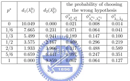
(25) Here E(log[1+. Pk. i=1 exp(ηit )]; F2,λ02 ). can be numerically evaluated by the method of the mul-. tivariate Gauss-Hermite integration. Finally, λ01 can be numerically evaluated by utilizing the Newton-Raphson method. We simulate an i.i.d. sample {y(1) , . . . , y(R) } of size R, e.g., R = 100 000, from the c.d.f. Fy;2,λ02 . Since all of λ01 , λ02 , and λn1 1 are known in a simulation study, we can numerically evaluate P ({φ∗λ0 ,λ0 (y) = 0}; F2,λ02 ) and P ({φ∗λn1 ,λn1 (y) = 0}; F2,λ02 ) by |{r : 1. 2. 1. 2. φ∗λ0 ,λ0 (y(r) ) = 0}|/R and |{r : φ∗λn1 ,λn1 (y(r) ) = 0}|/R, respectively. Since both λ01 and λ02 are 1. 2. 1. 2. unknown in a real problem, we can numerically evaluate P ({φ∗λˆ. ˆ. 1 ,λ2. φ∗λˆ. 1 (y. (r) ),λ ˆ 2 (y(r) ). (y) = 0}; F2,λ02 ) by |{r :. (y(r) ) = 0}|/R.. For the simulation study, consider the case where F = F2,λ02 with λ02 = (−1.450, −2.450, (1). (R). 1.273, −0.109, 0.565)T . We simulate an i.i.d. sample {θt , . . . , θt } of size R, e.g., R = 0(0). 100 000, from the c.d.f. F2,λ02 . Set λ1. 0(0). 00(0). ≡ λ1s ·λ1. 0(0). , where λ1s is the MME of λ1s proposed. in Shiau et al. (2005) and 00(0) λ1. R 1 X (r) θt . ≡ · R r=1. Iterating equation (8), we obtain λ01 = (5.771, 1.707, 0.884)T . Iterating equation (20), λn1 1 is obtained and shown in Table 2 for n1 ∈ {35, 70, 140}. Similarly, it is easily seen that ||λn1 1 − λ01 ||2 decreases as n1 increases, where ||λn1 1 − λ01 ||2 ≡ [(λn1 1 − λ01 )T (λn1 1 − λ01 )]1/2 . Finally, we obtain P ({φ∗λ0 ,λ0 (y) = 0}; F2,λ02 ) ≈ 0.021, P ({φ∗λn1 ,λn1 (y) = 0}; F2,λ02 ) ≈ 0.008, 1. and P ({φ∗λˆ. ˆ. 1 ,λ2. 2. 1. 2. (y) = 0}; F2,λ02 ) ≈ 0.014 which are all less than 0.5 and shown in Table 3.. Case 3 : F = p∗ · F1,λ∗1 + (1 − p∗ ) · F2,λ∗2 for some 0 < p∗ < 1, λ∗1 ∈ Λ1 , and λ∗2 ∈ Λ2 , 19.

(26) where p∗ · F1,λ∗1 + (1 − p∗ ) · F2,λ∗2 6∈ {Fu,λu : λu ∈ Λu and u ∈ {1, 2}}. We simulate an i.i.d. sample {y(1) , . . . , y(R) } of size R, e.g., R = 100 000, from the c.d.f. Fy . The initial value of λ0u for u ∈ {1, 2} can be obtained by the same methods in Case 1 and 2. Iterating equation (8), λ0u can be numerically evaluated. When d1 (λ01 ) ≤ d2 (λ02 ), we can numerically evaluate P ({φ∗λ0 ,λ0 (y) = 1}; F ), P ({φ∗λ35 ,λ35 (y) = 1}; F ), and P ({φ∗λˆ. 1 ,λ2. = 1}; F ) by |{r : φ∗λ0 ,λ0 (y(r) ) = 1}|/R, |{r : φ∗λ35 ,λ35 (y(r) ) = 1}|/R, and |{r : φ∗λˆ. 2 (y. 1. 1. 1. 2. 1. 2. 2. 1 (y. 2. (r) ),λ ˆ. ˆ. (y). (r) ). (y(r) ). = 1}|/R, respectively. When d1 (λ01 ) > d2 (λ02 ), we can numerically evaluate P ({φ∗λ0 ,λ0 (y) = 1. 0}; F ), P ({φ∗λ35 ,λ35 (y) = 0}; F ), and P ({φ∗λˆ 1. 2. |{r : φ∗λ35 ,λ35 (y(r) ) = 0}|/R, and |{r : φ∗λˆ 1. 2. 1 (y. ˆ. 1 ,λ2. (r) ),λ ˆ. 2. (y) = 0}; F ) by |{r : φ∗λ0 ,λ0 (y(r) ) = 0}|/R, 1. 2 (y. (r) ). 2. (y(r) ) = 0}|/R, respectively.. First, consider the case where F = p∗ ·F1,λ∗1 +(1−p∗ )·F2,λ∗2 for p∗ ∈ {1/6, 1/3, 1/2, 2/3, 5/6} with λ∗1 = (7, 2, 1)T and λ∗2 = (−1.450, −2.450, 1.273, −0.109, 0.565)T . Iterating equation (8), we can numerically evaluate λ0u for u ∈ {1, 2}. d1 (λ01 ), d2 (λ02 ), and the probability of choosing the wrong hypothesis for each of φ∗λ0 ,λ0 , φ∗λ35 ,λ35 , and φ∗λˆ 1. 2. 1. 2. ˆ. 1 ,λ2. are shown in Table 3.. It is easily seen from Table 3 that d1 (λ01 ) decreases and d2 (λ02 ) increases as p∗ increases. The probability of choosing the wrong hypothesis is less than 0.5 except for φ∗λˆ. ˆ. 1 ,λ2. with p∗ = 2/3.. Next, consider the case where F = p∗ ·F1,λ∗1 +(1−p∗ )·F2,λ∗2 for p∗ ∈ {1/6, 1/3, 1/2, 2/3, 5/6} with λ∗1 = (5.771, 1.707, 0.884)T and λ∗2 = (−1.450, −2.450, 1.273, −0.109, 0.565)T . Iterate equation (8), we can numerically evaluate λ0u for u ∈ {1, 2}. d1 (λ01 ), d2 (λ02 ), and the probability of choosing the wrong hypothesis for each of φ∗λ0 ,λ0 , φ∗λ35 ,λ35 , and φ∗λˆ 1. 2. 1. 2. ˆ. 1 ,λ2. are shown. in Table 4. Similarly, it is easily seen from Table 4 that d1 (λ01 ) decreases and d2 (λ02 ) increases as p∗ increases. The probability of choosing the wrong hypothesis is less than 0.5 except 20.

(27) for φ∗λ0 ,λ0 with p∗ = 1/2. The main reason is that d1 (λ01 ) (≈ 2.980) and d2 (λ02 ) (≈ 2.944) are 1. 2. nearly the same. Finally, we would like to investigate the results of the empirical Bayes process monitoring scheme proposed in Chen et al. (2004) and Chen et al. (2005) by ignoring the fact that the model used is only an approximate model. Let γ denote the false alarm rate, i.e., the probability that an out-of-control signal occurs when the manufacturing process is in control. Conventionally, γ is taken to 2Φ(−3) (≈ 0.0026998). ˆ u ’s in decreasing order of d(Fu,λ0 , Fu,λ )| For u ∈ {1, 2}, we order the 100 000 λ û u λu =λ u (≡ d(Fu,λ0u , Fu,λˆ u )), a measure of how close Fu,λˆ u is to Fu,λ0u in our study, where ´ ³ d F1,λ01 , F1,λ1 # k+1 # " " X¡ ¢£ ¡ ¢ ¡ ¢¤ Γ(λ1s ) Γ(λ01s ) λ01i − λ1i ψ λ01i − ψ λ01s + − log Qk+1 = log Qk+1 0 i=1 Γ(λ1i ) i=1 Γ(λ1i ) i=1 for λ1 ∈ Λ1 and ´ ³ d F2,λ02 , F2,λ2 =. 1 2. ¸ ½ · ´¾ ³ ¡ ¢ ¡ 0 ¢−1 ¡ ¢ |Σ| T −1 0 T 0 + E (ηt − µ) Σ (ηt − µ) − ηt − µ Σ ηt − µ ; F2,λ02 log |Σ0 |. for λ2 ∈ Λ2 . Set ξt ≡ Σ1/2 (ηt − µ0 ), µ0 ≡ Σ1/2 (µ − µ0 ), and V ≡ (Σ0 )1/2 Σ−1 (Σ0 )1/2 . Then. E. ´ ³¡ ¢T ¡ ¢ ξt − µ0 V ξt − µ0 ; F2,λ02. ´´ ³ ³¡ ¡ ¡ ¢¢ ¢¡ ¢T = tr V I + µ0 µ0T = tr V · E ξt − µ0 ξt − µ0 ; F2,λ02. 21.

(28) and ´ ³ d F2,λ02 , F2,λ2 = =. ó ´ ³ ³¡ ¡ ¢ ¢T ¡ ¢ 1n log (|Σ|) − log |Σ0 | + E ξt − µ0 V ξt − µ0 ; F2,λ02 − E ξtT ξt ; F2,λ02 2 o ¡ ¢ ¡ ¢ ¡ ¢T ¡ ¢ 1n log (|Σ|) − log |Σ0 | + tr Σ0 Σ−1 + µ − µ0 Σ−1 µ − µ0 − k . 2. Thus, we pick the MLE’s corresponding to the best 10th, 30th, 50th, 70th, and 90th percentiles of these 100 000 MLE’s based on this measure. For the true λu and each MLE picked, compute the in-control probability and the average run length ARL0 when the process is in control. When the process is out of control, compute the out-of -control probability and the average run length ARL1 . Consider the case where F = F1,λ01 with λ01 = (7, 2, 1)T . Utilizing model 2 with λ02 = (−1.450, −2.450, 1.273, −0.109, 0.565)T for monitoring, the in control probability and ARL0 ˆ 2 ’s are shown in Table 5. It is easily seen for λ02 and the best 10%, 30%, 50%, 70%, 90% λ from Table 5 that the γλ02 and all the γλˆ 2 are less than γ. When θt has an out of control ˜ 1 = (5, 3, 2)T different from the in-control c.d.f. F 0 . The out of control c.d.f. F1,λ˜ 1 with λ 1,λ1 ˆ 2 ’s are shown in probability and ARL1 for λ02 and the best 10%, 30%, 50%, 70%, 90% λ Table 6. Consider the case where F = F2,λ02 with λ02 = (−1.450, −2.450, 1.273, −0.109, 0.565)T . Utilizing model 1 with λ01 = (5.771, 1.707, 0.884)T for monitoring, the in control probability ˆ 2 ’s are shown in Table 7. It is and ARL0 for λ02 and the best 10%, 30%, 50%, 70%, 90% λ easily seen from Table 7 that the γλ01 and all the γλˆ 1 are larger than γ. 22.

(29) First, consider the case where F = p∗ ·F1,λ∗1 +(1−p∗ )·F2,λ∗2 for p∗ ∈ {1/6, 1/3, 1/2, 2/3, 5/6} with λ∗1 = (7, 2, 1)T and λ∗2 = (−1.450, −2.450, 1.273, −0.109, 0.565)T . Utilizing model 2 for monitoring, the in control probability and ARL0 for λ02 and the best 10%, 30%, 50%, ˆ 2 ’s are shown in Table 8. It is easily seen from Table 8 that the γ 0 and 70%, 90% λ λ2 all the γλˆ 2 are less than γ. Utilizing model 1 for monitoring, the in control probability ˆ 1 ’s are shown in Table 9. It and ARL0 for λ01 and the best 10%, 30%, 50%, 70%, 90% λ is easily seen from Table 9 that the γλ01 and all the γλˆ 1 are large than γ. When θt has an ˜1 = out of control c.d.f. F = p˜ · F1,λ˜ 1 + (1 − p˜) · F2,λ˜ 2 for p˜ ∈ {1/6, 1/3, 1/2, 2/3, 5/6} with λ ˜ 2 = (−0.583, −1.083, 1.787, −0.456, 1.271)T different from the in control (5, 3, 2)T and λ c.d.f. F = p∗ · F1,λ∗1 + (1 − p∗ ) · F2,λ∗2 . Utilizing model 2 for monitoring, the out of control ˆ 2 ’s are shown in probability and ARL1 for λ02 and the best 10%, 30%, 50%, 70%, 90% λ Table 10 and 11, respectively. Next, consider the case where F = p∗ ·F1,λ∗1 +(1−p∗ )·F2,λ∗2 for p∗ ∈ {1/6, 1/3, 1/2, 2/3, 5/6} with λ∗1 = (5.771, 1.707, 0.884)T and λ∗2 = (−1.450, −2.450, 1.273, −0.109, 0.565)T . Utilizing model 2 for monitoring, the in control probability and ARL0 for λ02 and the best 10%, ˆ 2 ’s are shown in Table 12. It is easily seen from Table 12 that 30%, 50%, 70%, 90% λ the γλ02 and all the γλˆ 2 are less than γ. Utilizing model 1 for monitoring, the in control ˆ 1 ’s are shown in Table probability and ARL0 for λ01 and the best 10%, 30%, 50%, 70%, 90% λ 13. It is easily seen from Table 13 that the γλ01 and all the γλˆ 1 are large than γ. When θt has ˜1 = an out of control c.d.f. F = p˜·F1,λ˜ 1 +(1− p˜)·F2,λ˜ 2 for p˜ ∈ {1/6, 1/3, 1/2, 2/3, 5/6} with λ ˜ 2 = (−0.583, −1.083, 1.787, −0.456, 1.271)T different from the in-control (5, 3, 2)T and λ 23.

(30) c.d.f. F = p∗ · F1,λ∗1 + (1 − p∗ ) · F2,λ∗2 . Utilizing model 2 for monitoring, the out of control ˆ 2 ’s are shown in probability and ARL1 for the λ02 and the best 10%, 30%, 50%, 70%, 90% λ Table 14 and 15, respectively.. 5. CONCLUSIONS AND FUTURE WORK. In the paper, we develop a model selection technique for categorical data in manufacturing process. Then an example of choosing two empirical Bayes models for categorical data is discussed. If F = p∗ ·F1,λ∗1 +(1−p∗ )·F2,λ∗2 , for p∗ ∈ [0, 1], λ∗1 ∈ Λ1 , and λ∗2 ∈ Λ2 , then the probability of choosing the wrong hypothesis are almost less than 0.5. For the process monitoring, since these two parametric models under consideration are only approximate models, the critical point is incorrect such that the probability of signaling out-of-control is different from the γ. What we want to do next is to utilize the resampling method to find an approximate critical point for monitoring.. 24.

(31) APPENDIX All of nodes and weights of the Hermite polynomial of 32 degrees are shown in the following table. This table is obtained from the following website: http://www.efunda.com/math/num integration/findgausshermite.cfm. No.i 1 2 3 4 5 6 7 8 9 10 11 12 13 14 15 16 17 18 19 20 21 22 23 24 25 26 27 28 29 30 31 32. abscissas xi −7.12581390983 −6.40949814928 −5.81222594946 −5.27555098664 −4.77716450334 −4.30554795347 −3.85375548542 −3.41716749282 −2.99249082501 −2.57724953773 −2.16949918361 −1.76765410946 −1.37037641095 −0.97650046359 −0.58497876544 −0.19484074157 0.19484074157 0.58497876544 0.97650046359 1.37037641095 1.76765410946 2.16949918361 2.57724953773 2.99249082501 3.41716749282 3.85375548542 4.30554795347 4.77716450334 5.27555098664 5.81222594946 6.40949814928 7.12581390983 25. weights wi 7.31067642754 × 10−23 9.23173653482 × 10−19 1.19734401957 × 10−15 4.21501019491 × 10−13 5.93329148347 × 10−11 4.09883215841 × 10−9 1.57416779440 × 10−7 3.65058512533 × 10−6 5.41658405999 × 10−5 5.36268365495 × 10−4 3.65489032677 × 10−3 1.75534288315 × 10−2 6.04581309559 × 10−2 1.51269734077 × 10−1 2.77458142303 × 10−1 3.75238352593 × 10−1 3.75238352593 × 10−1 2.77458142303 × 10−1 1.51269734077 × 10−1 6.04581309559 × 10−2 1.75534288315 × 10−2 3.65489032677 × 10−3 5.36268365495 × 10−4 5.41658405999 × 10−5 3.65058512533 × 10−6 1.57416779440 × 10−7 4.09883215841 × 10−9 5.93329148347 × 10−11 4.21501019491 × 10−13 1.19734401957 × 10−15 9.23173653482 × 10−19 7.31067642754 × 10−23.

(32) REFERENCES. 1. Abramowitz, M. and Stegun, I. A. (1964). Handbook of Mathematical Functions: with Formulas, Graphs, and Mathematical Tables. Dover Publications, New York.. 2. Agresti, A. (2002). Categorical Data Analysis, 2nd ed. John Wiley & Sons, New York.. 3. Carlin, B. P. and Louis, T. A. (2000). Bayes and Empirical Bayes Methods for Data Analysis, 2nd ed. Chapman & Hall/CRC, Boca Raton.. 4. Chen, C.-R., Shiau, J.-J. H., Liao, H.-H., and Feltz, C. J. (2004). A process monitoring technique for categorical data under the beta-binomial or Dirichlet-multinomial empirical Bayes model. Technical Report, Institute of Statistics, National Chiao Tung University, Hsinchu, Taiwan.. 5. Chen, C.-R., Shiau, J.-J. H., Lin, T.-Y., and Feltz, C. J. (2005). A process monitoring technique for categorical data under the transformed-normal-binomial or transformednormal-multinomial empirical Bayes model. Technical Report, Institute of Statistics, National Chiao Tung University, Hsinchu, Taiwan.. 6. Fahrmeir, A. and Tutz, G. (2001). Multivariate Statistical Modelling Based on Generalized Linear Models, 2nd ed. Springer-Verlag, New York.. 7. Gelman, A., Carlin, J. B., Stern, H. S., and Rubin, D. B. (2004). Bayesian Data Analysis, 2nd ed. Chapman & Hall/CRC, Boca Raton.. 26.

(33) 8. Johnson, N. L., Kotz, S., and Balakrishnan, N. (1997). Discrete Multivariate Distributions. John Wiley & Sons, New York.. 9. McCullagh, P. and Nelder, J. A. (1989). Generalized Linear Models, 2nd ed. Chapman and Hall, London.. 10. O’Hagan, A. and Forster, J. (2004). Kendall’s Advanced Theory of Statistics, Volume 2B: Bayesian Inference, 2nd ed. Arnold, London.. 11. Shiau, J.-J. H., Chen, C.-R., and Feltz, C. J. (2005). An empirical Bayes process monitoring technique for polytomous data. Quality and Reliability Engineering International, 21, 13-28.. 12. Yousry, M. A., Sturm, G. W., Feltz, C. J., and Noorossana, R. (1991). Process monitoring in real time: empirical Bayes approach - discrete case. Quality and Reliability Engineering International, 7, 123-132.. Table 1: λn2 1 and ||λn2 1 − λ02 ||2 for n1 ∈ {35, 70, 140} with λ02 = (−1.450, −2.450, 1.273, −0.109, 0.565)T . λn2 1 n1 35 (−1.430, −2.344, 1.475, −0.194, 0.862)T 70 (−1.435, −2.366, 1.423, −0.172, 0.798)T 140 (−1.440, −2.387, 1.376, −0.154, 0.741)T. 27. ||λn2 1 − λ02 ||2 0.385 0.296 0.218.

(34) Table 2: λn1 1 and ||λn1 1 − λ01 ||2 for n1 ∈ {35, 70, 140} with λ01 = (5.771, 1.707, 0.884)T . λn1 1 n1 35 (6.935, 1.991, 1.004)T 70 (6.779, 1.953, 0.990)T 140 (6.597, 1.909, 0.973)T. ||λn1 1 − λ01 ||2 0.229 0.172 0.121. Table 3: d1 (λ01 ), d2 (λ02 ), and the probability of choosing the wrong hypothesis for each of φ∗λ0 ,λ0 , φ∗λn1 ,λn1 , and φ∗λˆ ,λˆ for p∗ ∈ {0, 1/6, 1/3, 1/2, 2/3, 5/6, 1} with λ∗1 = (7, 2, 1)T , 1. 2. 1. 1. 2. 2. λ∗2 = (−1.450, −2.450, 1.273, −0.109, 0.565)T , T = 300, and n1 = . . . = nT = 35. p∗. d1 (λ01 ). d2 (λ02 ). 0 1/6 1/3 1/2 2/3 5/6 1. 10.049 7.665 5.499 3.575 1.933 0.659 0.000. 0.000 0.231 0.941 2.167 3.966 6.441 9.859. the probability of choosing the wrong hypothesis ∗ φ∗λˆ ,λˆ φ∗λn1 ,λn1 φλ0 ,λ0 1. 2. 0.021 0.071 0.189 0.409 0.317 0.097 0.007. 1. 2. 0.008 0.064 0.147 0.296 0.488 0.247 0.064. 1. 2. 0.014 0.041 0.100 0.219 0.589 0.351 0.127. Table 4: d1 (λ01 ), d2 (λ02 ), and the probability of choosing the wrong hypothesis for each of φ∗λ0 ,λ0 , φ∗λn1 ,λn1 , and φ∗λˆ ,λˆ for p∗ ∈ {0, 1/6, 1/3, 1/2, 2/3, 5/6, 1} with λ∗1 = 1. 2. 1. 1. 2. 2. (5.771, 1.707, 0.884)T , λ∗2 = (−1.450, −2.450, 1.273, −0.109, 0.565)T , T = 300, and n1 = . . . = nT = 35. p∗. d1 (λ01 ). d2 (λ02 ). the probability of choosing the wrong hypothesis φ∗λˆ ,λˆ φ∗λn1 ,λn1 φ∗λ0 ,λ0. 0 1/6 1/3 1/2 2/3 5/6 1. 10.049 7.290 4.930 2.980 1.466 0.433 0.000. 0.000 0.333 1.319 2.944 5.209 8.141 11.841. 0.021 0.085 0.249 0.515 0.211 0.049 0.004. 1. 28. 2. 1. 2. 0.008 0.072 0.172 0.340 0.429 0.190 0.049. 1. 2. 0.014 0.049 0.132 0.285 0.497 0.264 0.116.

(35) Table 5: γλ02 , γλˆ 2 , ARL0,λ02 , and ARL0,λˆ 2 for the best 10%, 30%, 50%, 70%, 90% of these 100 000 i.i.d. experiments in a decreasing order by d(F2,λ02 , F2,λˆ 2 ) with λ02 = (−1.450, −2.450, 1.273, −0.109, 0.565)T , T = 300, and n1 = . . . = nT = 35 when F = F1,λ01 with λ01 = (7, 2, 1)T . 90% 70% 30% 50% 10% γλˆ 2 γλˆ 2 γλˆ 2 γλˆ 2 γλˆ 2 γλ02 0.0005 0.0003 0.001 0.001 0.0003 0.001 90% 70% 50% 30% 10% ARL0,λ02 ARL0,λˆ 2 ARL0,λˆ 2 ARL0,λˆ 2 ARL0,λˆ 2 ARL0,λˆ 2 2073.867 2921.422 1280.703 1168.032 3826.315 1000.012. Table 6: Pout,λ0 ,λ˜ 1 , Pout,λˆ 2 ,λ˜ 1 , ARL1,λ0 ,λ˜ 1 , and ARL1,λˆ 2 ,λ˜ 1 for the 2 2 best 10%, 30%, 50%, 70%, 90% of these 100 000 i.i.d. experiments in a decreasing order by the d(F2,λ02 , F2,λˆ 2 ) with λ02 = (−1.450, −2.450, 1.273, −0.109, 0.565)T , T = 300, ˜ 1 = (5, 3, 2)T . and n1 = . . . = nT = 35 when F = F ˜ with λ 1,λ1. Pout,λ0 ,λ˜ 1 2 0.017 ARL1,λ0 ,λ˜ 1 2 60.267. 30% Pout,λˆ 2 ,λ˜ 1 0.024. 10% Pout,λˆ 2 ,λ˜ 1 0.012. 10% ARL1,λˆ 2 ,λ˜ 1 80.561. 30% ARL1,λˆ 2 ,λ˜ 1 42.014. 70% Pout,λˆ 2 ,λ˜ 1 0.009. 50% Pout,λˆ 2 ,λ˜ 1 0.024 50% ARL1,λˆ 2 ,λ˜ 1 41.456. 90% Pout,λˆ 2 ,λ˜ 1 0.027. 70% ARL1,λˆ 2 ,λ˜ 1 115.074. 90% ARL1,λˆ 2 ,λ˜ 1 36.492. Table 7: γλ01 , γλˆ 1 , ARL0,λ01 , and ARL0,λˆ 1 for the best 10%, 30%, 50%, 70%, 90% of these 100 000 i.i.d. experiments in a decreasing order by the d(F1,λ01 , F1,λˆ 1 ) with λ01 = (5.771, 1.707, 0.884)T , T = 300, and n1 = . . . = nT = 35 when F = F1,λ02 with λ02 = (−1.450, −2.450, 1.273, −0.109, 0.565)T . 10% 30% 50% 70% 90% γλˆ 1 γλˆ 1 γλˆ 1 γλˆ 1 γλˆ 1 γλ01 0.010 0.009 0.016 0.015 0.012 0.012 ARL0,λ01 97.912. 10% ARL0,λˆ 1 110.413. 30% ARL0,λˆ 1 62.723. 50% ARL0,λˆ 1 68.348. 29. 70% ARL0,λˆ 1 86.875. 90% ARL0,λˆ 1 83.515.

(36) Table 8: γλ02 , γλˆ 2 , ARL0,λ02 , and ARL0,λˆ 2 for the best 10%, 30%, 50%, 70%, 90% of these 100 000 i.i.d. experiments in a decreasing order by the d(F2,λ02 , F2,λˆ 2 ) with T = 300 and n1 = . . . = nT = 35 when F = p∗ · F1,λ∗1 + (1 − p∗ ) · = = (7, 2, 1) and λ∗2 ∈ {1/6, 1/3, 1/2, 2/3, 5/6} with λ∗1 F2,λ∗2 for p∗ T (−1.450, −2.450, 1.273, −0.109, 0.565) . p∗ 1/6 1/3 1/2 2/3 5/6. γλ02 0.002 0.002 0.002 0.001 0.001. 10% γλˆ 2 0.002 0.002 0.001 0.001 0.001. 30% γλˆ 2 0.002 0.003 0.001 0.001 0.001. 50% γλˆ 2 0.002 0.002 0.001 0.001 0.001. 70% γλˆ 2 0.002 0.002 0.003 0.002 0.001. 90% γλˆ 2 0.002 0.003 0.001 0.002 0.001. 90% 70% 50% 30% 10% p∗ ARL0,λ02 ARL0,λˆ 2 ARL0,λˆ 2 ARL0,λˆ 2 ARL0,λˆ 2 ARL0,λˆ 2 1/6 429.149 458.667 452.298 617.770 428.381 668.522 1/3 510.049 572.669 309.477 407.377 405.927 369.132 1/2 628.538 714.295 1096.739 828.135 316.158 681.330 2/3 818.737 1333.622 848.331 734.249 554.763 617.768 5/6 1173.996 1013.322 1345.436 1156.539 1151.260 689.321. 30.

(37) Table 9: γλ01 , γλˆ 1 , ARL0,λ01 , and ARL0,λˆ 1 for the best 10%, 30%, 50%, 70%, 90% of these 100 000 i.i.d. experiments in a decreasing order by the d(F1,λ01 , F1,λˆ1 ) with T = 300 and n1 = . . . = nT = 35 when F = p∗ · F1,λ∗1 + (1 − p∗ ) · = = (7, 2, 1) and λ∗2 ∈ {1/6, 1/3, 1/2, 2/3, 5/6} with λ∗1 F2,λ∗2 for p∗ T (−1.450, −2.450, 1.273, −0.109, 0.565) . p∗ 1/6 1/3 1/2 2/3 5/6. γλ01 0.010 0.008 0.007 0.006 0.004. 10% γλˆ 1 0.013 0.010 0.013 0.006 0.006. 30% γλˆ 1 0.011 0.009 0.008 0.006 0.003. 50% γλˆ 1 0.007 0.009 0.006 0.006 0.009. 70% γλˆ 1 0.008 0.008 0.006 0.005 0.004. 90% γλˆ 1 0.008 0.005 0.006 0.009 0.004. 90% 70% 50% 30% 10% p∗ ARL0,λ01 ARL0,λˆ 1 ARL0,λˆ 1 ARL0,λˆ 1 ARL0,λˆ 1 ARL0,λˆ 1 93.531 136.475 120.389 119.532 78.989 1/6 104.101 1/3 118.335 104.301 107.397 113.588 133.027 187.852 78.626 132.239 170.435 179.943 181.045 1/2 133.595 2/3 169.300 163.799 166.018 178.248 195.913 117.159 5/6 226.574 179.740 330.658 113.433 268.169 222.592. 31.

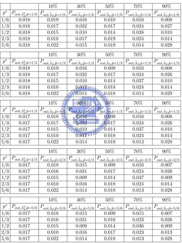
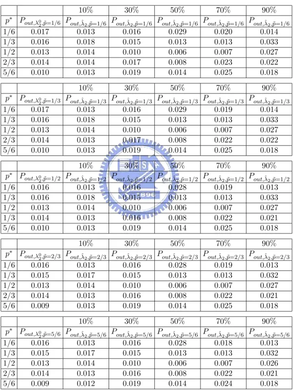
(38) Table 10: Pout,λ02 ,˜p and Pout,λˆ 2 ,˜p for the best 10%, 30%, 50%, 70%, 90% these 100 000 i.i.d. experiments in a decreasing order by the d(F2,λ02 , F2,λˆ 2 ) with p∗ {1/6, 1/3, 1/2, 2/3, 5/6}, T = 300, and n1 = . . . = nT = 35 when F ˜ 1 = (5, 3, 2)T and λ ˜2 p˜ · F1,λ˜ 1 + (1 − p˜) · F2,λ˜ 2 for p˜ ∈ {1/6, 1/3, 1/2, 2/3, 5/6} with λ T (−0.583, −1.083, 1.787, −0.456, 1.271) . 90% 70% 50% 30% 10% p∗ Pout,λ02 ,˜p=1/6 Pout,λˆ 2 ,˜p=1/6 Pout,λˆ 2 ,˜p=1/6 Pout,λˆ 2 ,˜p=1/6 Pout,λˆ 2 ,˜p=1/6 Pout,λˆ 2 ,˜p=1/6 0.008 0.016 0.010 0.016 0.019 0.018 1/6 0.027 0.024 0.017 0.032 0.017 0.018 1/3 0.010 0.038 0.014 0.010 0.015 0.018 1/2 0.014 0.024 0.019 0.017 0.010 0.018 2/3 0.029 0.014 0.019 0.015 0.022 0.018 5/6 10% p∗ 1/6 1/3 1/2 2/3 5/6. 1/6 1/3 1/2 2/3 5/6. 70%. 90%. Pout,λ02 ,˜p=1/3 Pout,λˆ 2 ,˜p=1/3 Pout,λˆ 2 ,˜p=1/3 Pout,λˆ 2 ,˜p=1/3 Pout,λˆ 2 ,˜p=1/3 Pout,λˆ 2 ,˜p=1/3 0.008 0.016 0.009 0.016 0.019 0.018 0.026 0.024 0.017 0.032 0.017 0.018 0.010 0.037 0.014 0.010 0.015 0.018 0.014 0.024 0.018 0.017 0.010 0.018 0.029 0.014 0.018 0.015 0.022 0.018 10%. p∗. 50%. 30%. 50%. 30%. 70%. 90%. Pout,λ02 ,˜p=1/2 Pout,λˆ 2 ,˜p=1/2 Pout,λˆ 2 ,˜p=1/2 Pout,λˆ 2 ,˜p=1/2 Pout,λˆ 2 ,˜p=1/2 Pout,λˆ 2 ,˜p=1/2 0.008 0.016 0.009 0.016 0.018 0.017 0.026 0.024 0.017 0.032 0.017 0.017 0.010 0.037 0.014 0.010 0.015 0.017 0.014 0.024 0.018 0.017 0.010 0.017 0.028 0.013 0.018 0.014 0.022 0.017. 90% 70% 50% 30% 10% p∗ Pout,λ02 ,˜p=2/3 Pout,λˆ 2 ,˜p=2/3 Pout,λˆ 2 ,˜p=2/3 Pout,λˆ 2 ,˜p=2/3 Pout,λˆ 2 ,˜p=2/3 Pout,λˆ 2 ,˜p=2/3 0.007 0.016 0.009 0.015 0.018 0.017 1/6 0.026 0.024 0.017 0.031 0.016 0.017 1/3 0.009 0.037 0.014 0.009 0.015 0.017 1/2 0.014 0.024 0.018 0.016 0.010 0.017 2/3 0.028 0.013 0.018 0.014 0.022 0.017 5/6 10% p∗ 1/6 1/3 1/2 2/3 5/6. 50%. 30%. 70%. 90%. Pout,λ02 ,˜p=5/6 Pout,λˆ 2 ,˜p=5/6 Pout,λˆ 2 ,˜p=5/6 Pout,λˆ 2 ,˜p=5/6 Pout,λˆ 2 ,˜p=5/6 Pout,λˆ 2 ,˜p=5/6 0.007 0.015 0.009 0.015 0.018 0.017 0.026 0.023 0.016 0.031 0.016 0.017 0.009 0.036 0.014 0.009 0.015 0.017 0.013 0.023 0.017 0.016 0.010 0.017 0.028 0.013 0.018 0.014 0.022 0.017 32. of ∈ = =.

(39) Table 11: ARL1,λ02 ,˜p and ARL1,λˆ 2 ,˜p for the best 10%, 30%, 50%, 70%, 90% of these 100 000 i.i.d. experiments in a decreasing order by the d(F2,λ02 , F2,λˆ 2 ) with p∗ ∈ {1/6, 1/3, 1/2, 2/3, 5/6}, T = 300, and n1 = . . . = nT = 35 when F = p˜ · ˜ 1 = (5, 3, 2)T and λ ˜2 = F1,λ˜ 1 + (1 − p˜) · F2,λ˜ 2 for p˜ ∈ {1/6, 1/3, 1/2, 2/3, 5/6} with λ T (−0.583, −1.083, 1.787, −0.456, 1.271) . 90% 70% 50% 30% 10% p∗ ARL1,λ02 ,˜p=1/6 ARL1,λˆ 2 ,˜p=1/6 ARL1,λˆ 2 ,˜p=1/6 ARL1,λˆ 2 ,˜p=1/6 ARL1,λˆ 2 ,˜p=1/6 ARL1,λˆ 2 ,˜p=1/6 129.189 61.277 104.086 63.070 53.492 56.099 1/6 37.370 41.165 57.219 30.879 58.840 56.099 1/3 99.071 26.646 71.053 102.242 64.748 56.099 1/2 69.115 41.032 53.786 58.573 98.407 56.099 2/3 34.400 72.064 53.632 67.726 44.761 56.099 5/6 10%. 30%. 50%. 70%. 90%. p∗. ARL1,λ02 ,˜p=1/3 ARL1,λˆ 2 ,˜p=1/3 ARL1,λˆ 2 ,˜p=1/3 ARL1,λˆ 2 ,˜p=1/3 ARL1,λˆ 2 ,˜p=1/3 ARL1,λˆ 2 ,˜p=1/3 131.093 62.250 105.968 63.773 54.063 56.886 1/6 37.813 41.538 58.061 31.224 59.566 56.886 1/3 101.090 26.864 71.634 103.591 65.411 56.886 1/2 70.506 41.509 54.676 59.329 99.995 56.886 2/3 34.747 73.222 54.315 68.392 45.038 56.886 5/6 10%. 30%. 50%. 70%. 90%. p∗. ARL1,λ02 ,˜p=1/2 ARL1,λˆ 2 ,˜p=1/2 ARL1,λˆ 2 ,˜p=1/2 ARL1,λˆ 2 ,˜p=1/2 ARL1,λˆ 2 ,˜p=1/2 ARL1,λˆ 2 ,˜p=1/2 133.053 63.255 107.918 64.492 54.646 57.695 1/6 38.266 41.919 58.927 31.577 60.310 57.695 1/3 103.192 27.086 72.224 104.976 66.087 57.695 1/2 71.954 41.997 55.596 60.105 101.634 57.695 2/3 35.100 74.418 55.017 69.072 45.318 57.695 5/6 90% 70% 50% 30% 10% p∗ ARL1,λ02 ,˜p=2/3 ARL1,λˆ 2 ,˜p=2/3 ARL1,λˆ 2 ,˜p=2/3 ARL1,λˆ 2 ,˜p=2/3 ARL1,λˆ 2 ,˜p=2/3 ARL1,λˆ 2 ,˜p=2/3 135.073 64.292 109.942 65.227 55.242 58.528 1/6 38.730 42.307 59.820 31.938 61.072 58.528 1/3 105.383 27.313 72.825 106.399 66.778 58.528 1/2 73.463 42.497 56.547 60.901 103.328 58.528 2/3 35.461 75.654 55.736 69.765 45.602 58.528 5/6 10%. 30%. 50%. 70%. 90%. p ARL1,λ02 ,˜p=5/6 ARL1,λˆ 2 ,˜p=5/6 ARL1,λˆ 2 ,˜p=5/6 ARL1,λˆ 2 ,˜p=5/6 ARL1,λˆ 2 ,˜p=5/6 ARL1,λˆ 2 ,˜p=5/6 137.155 65.364 112.044 65.979 55.852 59.385 1/6 39.206 42.702 60.740 32.307 61.855 59.385 1/3 107.670 27.542 73.435 107.860 67.484 59.385 1/2 75.036 43.009 57.531 61.718 105.080 59.385 2/3 35.829 76.931 56.475 70.471 45.889 59.385 5/6 33.

(40) Table 12: γλ02 , γλˆ 2 , ARL0,λ02 , and ARL0,λˆ 2 for the best 10%, 30%, 50%, 70%, 90% of these 100 000 i.i.d. experiments in a decreasing order by the d(F2,λ02 , F2,λˆ 2 ) with T = 300 and n1 = . . . = nT = 35 when F = p∗ · F1,λ∗1 + (1 − p∗ ) · F2,λ∗2 for p∗ ∈ {1/6, 1/3, 1/2, 2/3, 5/6} with λ∗1 = (5.771, 1.707, 0.884) and λ∗2 = (−1.450, −2.450, 1.273, −0.109, 0.565)T . p∗ 1/6 1/3 1/2 2/3 5/6. γλ02 0.002 0.002 0.001 0.001 0.001. 10% γλˆ 2 0.002 0.002 0.001 0.001 0.001. 70% 50% 30% γλˆ 2 γλˆ 2 γλˆ 2 0.002 0.004 0.004 0.002 0.001 0.001 0.002 0.001 0.002 0.001 0.0004 0.001 0.001 0.001 0.002. 90% γλˆ 2 0.001 0.004 0.003 0.002 0.001. 90% 70% 50% 30% 10% p∗ ARL0,λ02 ARL0,λˆ 2 ARL0,λˆ 2 ARL0,λˆ 2 ARL0,λˆ 2 ARL0,λˆ 2 1/6 470.175 595.580 443.966 276.241 239.030 769.612 1/3 592.735 416.511 536.236 846.050 970.737 224.911 1/2 756.675 813.934 649.492 856.887 508.406 305.835 2/3 955.090 959.679 1040.847 2301.318 1769.913 426.967 5/6 1447.122 1089.188 694.365 976.435 504.247 831.356. 34.

(41) Table 13: γλ01 , γλˆ 1 , ARL0,λ01 , and ARL0,λˆ 1 for the best 10%, 30%, 50%, 70%, 90% of these 100 000 i.i.d. experiments in a decreasing order by the d(F1,λ01 , F1,λˆ 1 ) with T = 300 and n1 = . . . = nT = 35 when F = p∗ · F1,λ∗1 + (1 − p∗ ) · F2,λ∗2 for p∗ ∈ {1/6, 1/3, 1/2, 2/3, 5/6} with λ∗1 = (5.771, 1.707, 0.884) and λ∗2 = (−1.450, −2.450, 1.273, −0.109, 0.565)T . p∗ 1/6 1/3 1/2 2/3 5/6. γλ01 0.009 0.008 0.006 0.005 0.004. 10% γλˆ 1 0.012 0.014 0.011 0.005 0.006. 30% γλˆ 1 0.008 0.009 0.008 0.010 0.005. 50% γλˆ 1 0.008 0.008 0.008 0.007 0.004. 70% γλˆ 1 0.011 0.006 0.006 0.004 0.004. 90% γλˆ 1 0.01 0.005 0.006 0.004 0.003. 90% 70% 50% 30% 10% p∗ ARL0,λ01 ARL0,λˆ 1 ARL0,λˆ 1 ARL0,λˆ 1 ARL0,λˆ 1 ARL0,λˆ 1 86.373 92.973 86.314 131.813 117.975 1/6 111.595 69.299 106.714 127.448 155.697 182.420 1/3 129.723 87.955 133.345 128.392 168.520 162.005 1/2 154.883 2/3 192.150 208.536 102.868 138.559 232.638 244.044 5/6 253.034 164.246 188.869 259.491 274.559 313.108. 35.