驅動壓電式材料之多級放大電路架構研究

國

立

交

通

大

學

機械工程系

博

士

論

文

驅動壓電式材料之多級放大電路架構研究

Multi-Level Amplifier for Driving Piezoelectric Loads

研 究 生：童永成

指導教授：成維華 教授

驅動壓電式材料之多級放大電路架構研究

Multi-level Amplifier for Diving Piezoelectric Loads

研 究 生：童永成 Student：Yung-Cheng Tung 指導教授：成維華 Advisor：Wei-Hua Chieng 國 立 交 通 大 學 機 械 工 程 系 博 士 論 文 A Dissertation

Submitted to Department of Mechanical Engineering College of Engineering

National Chiao Tung University in Partial Fulfillment if the Requirements

for the Degree of Doctor of Philosophy

in

Mechanical Engineering July 2008

Hsinchu, Taiwan, Republic of China

驅動壓電式材料之多級放大電路架構研究 研究生 : 童 永 成 指導教授 : 成 維 華 教授 國立交通大學機械工程研究所 摘要 本研究提出一多級式放大電路架構用以驅動壓電式負載，此放大器利用 多級浮動訊號模組的疊加，產生一高電壓增益的輸出。文中首先介紹壓電 式負載放大器電路的特性以及研究方法，隨後藉由多級式放大電路架構的 分析及模擬，來探討此電路模型的可行性。此多級式放大電路系統，各級 供應相同的輸出電壓以及電流，系統總功率消耗平均分配至各級電路當 中，以致於多級式放大電路擁有高功率輸出的特點。文中提出一由六級浮 動訊號模組所組成的電路原型，用以實現高輸入頻率以及不同電容式負載 下的精密線性操作。其頻寬約為 100 KHz、並可在 400V 的輸出擺幅下驅動 0.1μF 的電容式負載；電路的迴轉率(Slew Rate) 高達 115 V/μs，最大 輸出電流為±2.6 A。

Multi-level Amplifier for Driving Piezoelectric Loads

Student : Yung-Cheng Tung Advisor : Dr. Wei-Hua CHieng Department of Mechanical Engineering

National Chiao Tung University

Abstract

This study proposes a multi-level amplifier with connecting floating signal modules in series to drive piezoelectric devices. The amplifier generates a high voltage gain by summing the individual module gains. In the first instance this literature introduces the characteristic and various researching methods of driving piezoelectric loadings. Then the feasibility of multi-level amplifier topology will be discussed by simulations and analyses. Multi-level amplifier provides a means of achieving high power, and can divide the total power dissipation among the modules, because each module delivers the same output voltage and current. A prototype circuit that consists of six floating signal modules exhibits precise linear operation over a wide range of input frequencies and capacitive loads. The circuit provides a 400V output swing with a corner frequency of around 100 kHz at a driving capacitive load of 0.1 μF. The slew rate is as high as 115 V/μs and the maximum output current is ±2.6 A.

致 謝 時間似白駒過隙，學生永成師事成維華老師已近十年，期間諄諄教誨， 無論課業上，抑或是生活上，老師亦師亦友的相伴，著實是學生在求學生 涯上的重要支柱。本論文的完成，感謝成維華老師一路上不厭其煩的教導， 以及包容。 感謝每位口試委員的指正以及教導，使學生得以順利完成本論文寫作。 求學期間，感謝中山科學研究院楊培基博士、陶吉文博士、黃志方博士 以及各位先進的協助指導，開拓學生在機械領域上的視野。感謝游武璋學 長長期以來的教導，使學生得以學習其它領域的知識，並開啟學習的道路。 感謝鄭時龍學長無私的指正教導，使學生在論文發表上得以一切順遂。感 謝張仰宏、楊嘉豐、黃旭生、潘怡仁以及黃柏瑞同學在學生求學生涯所提 供的一切協助以及相互砥礪。感謝吳秉霖、鄭斌佐、呂昆樺、張淦垚、黃 建成、曹明亮以及實驗室諸位學弟的相互支援與鼓勵。 感謝我的父母親，對學生無私且盡其所能的奉獻，讓學生得以無後顧之 憂的完成學業。最後，感謝英如近十年來的相知相守，跟一路上的支持鼓 勵。 衷心將此學位的榮耀獻與協助過學生的各位，謝謝。

Contents 摘要………i Abstract………..ii 致謝……….…...iii Contents………iv List of Figures………....vi List of Tables………...………..ix Nomenclatures………....x CHAPTER 1 INTRODUCTION……….………...1 1.1 General Introduction……….………1

1.2 Characteristics and Principles of Piezoelectric Actuators……….1

1.3 Driving in Current / Charge Amplifier……….3

1.4 Driving in Voltage Amplifier……….6

1.4.1 Switching Amplifier ……….. 7

1.4.2 Linear Amplifier………..………. 10

1.5 Controlling Strategy for Hysteresis Compensation ……….. 11

CHAPTER 2 MULTI-LEVEL AMPLIFIER………..12

2.1 Introduction………12

2.2 Cascade Amplifier………13

CHAPTER 3 INDIRECT-FLOATING CASCADED TOPOLOGY…….16

3.1 Difference Amplifier………….………..…. 16

3.2 Balanced Isolated Floating Difference Amplifier (BIFDA)…………. 18

3.3 Multi-Level Balanced Isolated Floating Difference Amplifier (MBIFDA) ……….... 20

3.4 Frequency Response Due to Capacitive Loads………..…. 22

3.5 Differential-Mode Gain in Single Level Amplifier………. 23

3.6 Differential-Mode Gain in Multi Level Amplifier………….…………. 26

4.1 Balanced Isolated Floating Difference Amplifier (BIFDA)……… 27 4.2 Multi-Level Balanced Isolated Floating Difference Amplifier (MBIFDA)……….…...………… 27

CHAPTER 5 SIMULATIONS AND EXPERIMENTAL RESULTS....30 5.1 Experimental Setup………..………30

5.2 Results of the Simulation and Experiment……..……….31 5.2.1 Time-Domain Response………..32 5.2.2 Frequency-Domain Response without External/Isolated Resistor..34 5.2.3 Frequency-Domain Response with External/Isolated Resistor……34 5.3 Isolated Power Supply Unit……….……….37

CHAPTER 6 CONCLUSIONS….………39 REFERENCES………41

List of Figures

Figure 1.1 Measured extension of piezoelectric actuator (a) Against applied voltage, (b) Against applied charge [5]…………... 48

Figure 1.2 Generic current source [7]……….. 49

Figure 1.3 Simplified schematic of a compliance feedback current amplifier[7] ….. ……… 49 Figure 1.4 Principle of driving method by using current pulse (a)

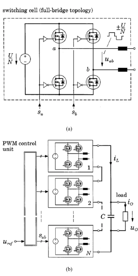
configuration of circuit, (b) displacement [11]…………... 50 Figure 1.5 (a) Inverter block diagram, (b) Full- Bridge inverter [13].. 51 Figure 1.6 Basic circuit topology of the multicell multilevel

switch-mode power amplifier (a) Single switch cell (full-bridge topology), (b) Total multistage amplifier system [15]... 52 Figure 1.7 Wave shapes of interleaved triangular carrier signals for a

multicell (N = 4) switched-mode amplifier [15]... 53 Figure 1.8 Basic circuit topology of linear amplifier with power

stage [19]... 54 Figure 1.9 A pair of bridge-connected power op amps drive the

piezoelectric actuator [20]……….. 55

Figure 2.1 The difference amplifier………. 56

Figure 2.2 Output signals of difference amplifier of different power

supply rail………... 56

Figure 2.3 Isolated floating difference amplifier (IFDA)………….... 57 Figure 2.4 BIFDA in direct-floating cascaded topology……..……... 58 Figure 2.5 Multi-level floating amplifier (a) Indirect-floating

cascaded topology, (b) Direct-floating cascaded topology 59 Figure 2.6 Gain principle of multi-level floating amplifier (a)

cascaded topology………... 60 Figure 3.1 BIFDA module in indirect-floating cascaded topology... 61

Figure 3.2 Flow path of multi-level floating amplifier in

indirect-floating cascaded topology………... 62

Figure 3.3 MBIFDA in indirect-floating cascaded topology……...… 63 Figure 3.4 Equivalent circuit of the difference amplifier with

nonzero output resistance and capacitive load……… 64

Figure 4.1 MBIFDA in direct-floating cascaded topology…..……… 65

Figure 5.1 (a)Experimental setup of direct-floating cascaded

topology……….. 66 Figure 5.1 (b)Experimental setup of indirect-floating cascaded

topology ………. 66 Figure 5.2 Contour plots of the damping ratio and nature frequency 67 Figure 5.3 Input and output signals of each level in six-level

amplifier……….. 68 Figure 5.4 Six-cell amplifier based on the 20 KHz sinusoidal input

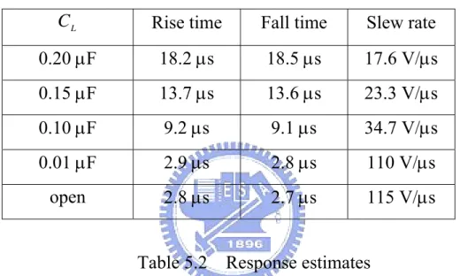
signal (a) Time response, (b) Power dissipation ……….... 69 Figure 5.5 Rise and fall times of the six-level amplifier under

various capacitive loads (a) IsSpice analysis results, (b)

Experimental results ……….. 70

Figure 5.6 Frequency response of direct-floating cascaded circuit topology without external/isolated resistance in six levels (a) Matlab® simulation (A) CL = 10pF, (B) CL = 10nF, (C) CL = 50nF, and (D) CL = 102nF ………... 71 (b) Experimental results: outputs on individual levels of MBIFDA based on the zero loading test ……… 71 (c) Experimental Result: frequency responses based on difference capacitive loadings……… 72

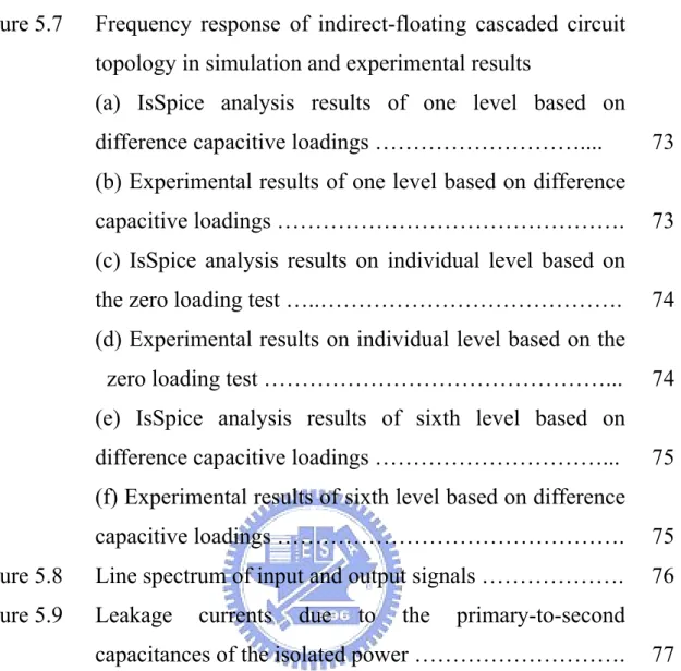
Figure 5.7 Frequency response of indirect-floating cascaded circuit topology in simulation and experimental results

(a) IsSpice analysis results of one level based on

difference capacitive loadings ……….... 73

(b) Experimental results of one level based on difference capacitive loadings ………. 73 (c) IsSpice analysis results on individual level based on the zero loading test …..………. 74 (d) Experimental results on individual level based on the

zero loading test ………... 74 (e) IsSpice analysis results of sixth level based on

difference capacitive loadings ………... 75

(f) Experimental results of sixth level based on difference capacitive loadings ………. 75

Figure 5.8 Line spectrum of input and output signals ………. 76

Figure 5.9 Leakage currents due to the primary-to-second

capacitances of the isolated power ………. 77

List of Tables

Table 1.1 Catalog of stack type piezo actuators [2] ………... 45

Table 4.1 Multi-level linear power amplifier specification ………... 46

Nomenclature

d , o

A , A_o,cm = Open-loop differential mode gain and common mode gain,

respectively d

, CL

A , A_CL,cm = Close-loop differential mode gain and common mode gain,

respectively d

, iso

A , A_iso,cm = Differential and common mode gain of the isolation amplifier,

respectively L

C = Capacitive load

max

f = The maximum operational frequency of piezoelectric actuator

0

f = Resonant frequency of unload actuator

i = The ithlevel of multi-level amplifier )

s (

I_L = Load current of current amplifier in s domain

) s (

I_LC = Actual Current follow through the load capacitor of current

amplifier in s domain T

k = Piezoelectric actuator stiffness

eff

m = Efficient mass applied to the actuator

max

P = The maximum peak power delivered to loads

L

q& ,q _L = The applied charge to piezoelectric load and its differentiation in

s domain L

R = Resistive load

o

R = Open-loop output resistance of the amplifier

s

R = Isolation resistance / Sensing resistor used in current amplifier

+

V , V₋ = Voltages at the non-inverting and inverting input terminals of

the amplifier, respectively b

V = Reference / Biased ground potential of the floating signal

d , in

V , V_in,cm = Differential mode and common mode input voltages,

respectively max

V = The maximum output voltage swing of amplifier

P P

V ₋ = Peak to peak driving voltage of piezoelectric actuator

+

iso , out

V , V_out− _,iso = Positive and negative differential output voltages of the isolation

amplifier, respectively p

, out

V , V_out,n = Output voltages of the floating signal module at non-inverting

and inverting terminals, respectively

) s (

V_ref = Reference voltage of current amplifier in s domain

o , CL

Z = Close-loop output impedance of the amplifier

) s (

A_o,d = Frequency response of the open-loop differential mode gain )

0 (

A_o,d = Differential mode gain at low frequency c

ω = Cut-off frequency

d , o

ω = Dominant pole frequency of the amplifier

n

ω = Natural frequency of the system

Chapter 1 Introduction

1.1 General Introduction

Piezoelectric devices or actuators have been used as positioners or driving motors in many fields such as optics, precision machining and fluid control as well as in optical disk drives, because they offer compactness, high energy density, rapid response and controllable displacement down to nanometers or less. The advantages that piezoelectric actuators offer are the absence of friction that exists in other actuators [1]. This dissertation introduces and proposes a novel circuit concept of driving piezoelectric actuators and two circuit topologies derived from this conception. At the beginning of this dissertation, the characteristic and principle of piezoelectric actuator will be introduced. Two fundamental sorts of driving amplifier, current/charge amplifier and voltage amplifier, and control methods will be introduced in section 1.3, 1.4 and 1.5.

1.2 Characteristics and Principles of Piezoelectric Actuators

The main characteristics of piezoelectric actuators are : extremely high resolution in the nanometer range, high bandwidth up to several kilohertz range, a large force up to a few tons, and very short travel in the sub-millimeter range [2]. Application areas of piezoelectric actuators include: micromanipulation, micro-assembly, add-ons for high-precision cutting machinery and as secondary actuators in macro/micro-motion systems such as dual-stage hard-disk drives. Such actuators are assembled from thin, laminar wafers of ceramic material, electrically connected in parallel. Increasing the voltage increases the length of the stack to a maximum strain for typical maximum input voltage. The applied voltage depends on the thickness of the ceramic and on its material properties. It typically ranges from a few tens of volts to a few hundred volts. The reactive powers induced by the highly capacitive characteristics of the actuators will

detrimentally affect the driving amplifiers [3].

As discussed in [3] and references therein, a piezoelectric actuator behaves as a capacitor when operated well below the resonant frequency. Piezoelectric stack actuators are assembled with thin, laminar wafers of electro-active ceramic material electrically connected in parallel. The equivalent capacitance of piezoelectric stack actuator is N times the capacitance of single layer. And the resonant frequency of piezoelectric stack actuators can be described as

eff T m k f

π

where f₀ [Hz] is the resonant frequency of unloaded actuator, k_T [N/m] is

the piezoelectric actuator stiffness and m_eff [Kg] is the efficient mass applied

to the actuator. The stiffness of a solid body depends on Young’s modulus of the material. Stiffness is normally expressed in terms of the spring constant k , _T

which describes the deformation of the body in response to an external force. Then the capacitance of actuator increases as the number of layer or the electrode surface area increases, a reasonable consideration is that the mass of actuator will also increase. This increasing mass will decrease the resonant frequency of actuator as eq. (1.1) under the condition that they have the same stiffness. So this is why all the product catalogs [3], [4] provided by manufacturers of the piezoelectric stack actuator show a trend that the lager capacitance actuator have a less resonant frequency, as shown in Table-1.1. The capacitance varies from tens nano–farad to tens micro-farad, and the resonant frequency from hundreds kHz to tens kHz.

Piezoelectric stack actuators are applied in many areas, like fiber optics, stabilizing mechanical arrangements, and kilo-hertz scanning and micro-positioning. From the view of application, most of them are operated in

the positioning modes, that piezoelectric actuators are operated well below their resonant frequencies. To sum up that be mentioned above, alternative application of piezoelectric stack actuator is high frequency with low capacitance or low frequency with high capacitance.

And then from the view of power, the delivered peak power [3] , P_max, to

load for sinusoidal operation is

max max

max CV V f

P ≈

π

where C is the capacitance of piezoelectric stack actuator, V_max is the

maximum output voltage swing of amplifier, V_p−p is the peak to peak drive

voltage and f_max is the operational frequency.

1.3 Driving in Current / Charge Amplifier

Several approaches of driving circuit topology have been proposed to reduce the inherent hysteretic nonlinearity by driving piezoelectric actuators with charge or current, rather than voltage [5]-[8]. As mentioned in [5] and referred therein, piezoelectric ceramics are ferroelectric materials and for this reason they are fundamentally nonlinear in their response to applied electric fields, showing hysteresis and also time-dependent creep. Such effects become increasingly noticeable the higher the electric field strength and the higher the piezoelectric sensitivity of the material. C. V. Newcomb et al. in 1982 [5] found that if the extension of such an actuator is plotted as a function of applied charge rather than applied voltage, hysteresis and creep virtually disappear and the characteristic becomes much more linear. Therefore, C. V. Newcomb et al. proposed charge drive for piezoelectric ceramic actuators as a means of improving their behavior as Fig. 1.1 shows.

had been proposed as Fig. 1.2. In the Laplace domain, at frequencies well within the bandwidth of the control loop, the load current I_L(s) is equal to

) ( / ) (s Z s V_{ref s} . If Z_s(s) is a resistor R , _s s ref L s V s R I ( )= ( )/ (1.3)

i.e., we have a current amplifier with gain 1/R_s A/V. If Z_s(s) is a capacitor

s C , s C s V s I q&_L = _L( )= _ref( ) _s (1.4) s ref L V s C q = ( ) (1.5)

i.e., we have a charge amplifier with gain C_s Columbs/V.

The foremost difficulty in employing such devices to drive highly capacitive loads is that of DC current or charge offsets. Inevitably, the voltage measured across the sensing impedance will contain a non-zero voltage offset; this and other sources of voltage or current offset in the circuit will result in a net output offset current or charge. As a capacitor integrates DC current, the uncontrolled output voltage will tend towards infinity and saturate at the power supply rails. Any offset in v_o limits the compliance range of the current source

and will eventually cause saturation. To limit the DC impedance of the load, i.e., limiting the DC compliance offset for a certain output offset current, a parallel

resistance is often used. With _L

L

L R

s C s

Z ( )= 1 || , the actual current I_LC(s)

following through the load capacitor is now,

L L L LC C R s s s I s I 1 ) ( ) ( + = (1.6)

Additional dynamics have been added to the current source, the transfer function now contains a high-pass filter with cutoff

L L c C R 1 =

ω

L L s ref LC C R s s R s V s I 1 1 ) ( ) ( + = (1.7)

In contrast to the infinite DC impedance of a purely capacitive load, the load impedance now flattens out towards DC at

ω

impedance of R_L. Thus, a DC offset current of i_dc results in a compliance

offset of v_dc =i_dcR_L. In a typical piezoelectric driving scenario, with C = _L

100nF, and i_dc =1

μ

compliance offset to 1 V. Refer to Eq. (1.7), phase lead exceeds 5 degrees below 18 Hz. Such poor low frequency response precludes the use of current amplifiers in applications requiring accurate low frequency tracking.

The compliance feedback current amplifier [6], [7] and another driving method [8] proposed by A. J. Fleming et al. discussed mainly how to estimate the DC offsets and a perfect result had been verified. As Fig. 1.3 shows, a compliance feedback current amplifier had been presented which is modified from the traditional structure of the current amplifier in Fig. 1.2, and consists of three stages - the differential input stage, the transconductance stage, and the output current stage. With such compliance feedback, current amplifier can efficiently estimate the DC offset and achieve excellent ultra-low frequency tracking upto 100 mHz. For high power current and charge amplifier, A. J. Fleming et al. suggested that the output stage be replaced with a PWM inverter, but a PWM controlled DC-AC inverter will limit the high frequency bandwidth of the amplifier, thus the output signal contains switching noise and current ripple.

Due to the uncontrolled nature of the output voltage, circuit offsets generally result in the load capacitor being charged up. Saturation and distortion occur when the output voltage reaches the power supply rails. The stated

complexity invariably refers to additional circuitry required to avoid charging of the capacitor. Another popular scheme is to short the loading circuit, or periodically discharge the loading capacitance and reset the DC voltage to ground during handling [9], [10]. The resulting loads induce undesirable high-frequency disturbance and considerably distort the control signal that is applied to the piezoelectric load.

K. Furutani et al. [11] in 2006, proposed a driving method by using current pulses, which aimed at the precise displacement control. This method applied pulse density modulation as shown in Fig. 1.4 and composed of a complex feedback loop with high resolution DAC, DSP and PID controller to achieve a performance in displacement as well as to use the voltage linear amplifier. But the operational frequency also ranges in the low frequency as the results presented by A. J. Fleming et al. [8].

1.4 Driving in Voltage Amplifier

Comparing with current or charge driving, voltage amplifiers can also be used to drive piezoelectric actuators because they can precisely generate any driving waveforms. Two topologies of amplifiers have been realized for driving piezoelectric actuators [12], [13]. One is based on switching and the other is a linear amplifier. As mentioned in [12] and references therein, N. Vujic et al. in 2002, proposed a comparison of linear and switching drive amplifiers for piezoelectric actuators. Therein, the well-known analyses are that the linear amplifiers consume significantly more power than the switching amplifiers. The power dissipations of the linear amplifiers increase with the increasing frequency because the capacitors draw more currents at higher frequency. The switching amplifiers show approximately constant power consumption over frequency because they recycle the current through storage capacitors. The constant power consumption represents (small) fixed losses in the amplifiers.

The following paragraphs 1.4.1 and 1.4.2 introduce both switching and linear amplifiers individually and make the comparison between each other.

1.4.1 Switching Amplifier

In a switching amplifier [13]-[15], a setup stage is initially adopted to generate the constant high voltage required by the piezoelectric actuator. The second stage is a half or full bridge as Fig. 1.5 shown in reference [13], which delivers the output voltage to the actuator as dictated by the reference signal. The output voltage is synthesized by appropriately controlling the power transistors using the pulse width modulator. The switches of the power transistors cause a ripple voltage on the top of these mean waveforms. This ripple voltage acts as a disturbance signal on the actuator, causing high-frequency excitation and undesired heating in the actuator. The ripple noise may be reduced by increasing the switching frequency. However, increasing the switching frequency increases the switching numbers of transistor as well as the switching losses in the power transistors. The switching frequency is typically held constant in a pulse width modulation (PWM) controller and is set to be between a few ten kilohertz and a few hundred kilohertz (20~100 kHz). The bandwidth of the switching amplifier is limited because the signal frequency must be much lower than the switching frequency. For a practical realization and application, the bandwidth of the signal to be amplified must be limited to ten percentage of the switching frequency. In addition the blanking time derived from the bridge circuit of switching amplifier will induce nonlinear outputs [16], and the switching harmonic frequency will impact to the quality of the output signal more or less.

Here, a brief discussion for the influence of blanking time would be introduced below. Referring to Fig. 1.5(b), the combination of T1 and T2 switches is the so-called one leg [16] of the full-bridge inverter, and T3/T4

composes the other leg. The turn-on of the other switch in that inverter leg is delayed by a blanking timet_Δ, which is conservatively chosen to avoid a “shoot

through” or cross-conduction current through the leg. This blanking time is chosen to be just a few microseconds for fast switching devices like MOSFETs and larger for slower switching devices. Therefore, the distortion or nonlinear induced from blanking time is explainable and reasonable. Then a load current is assumed to be sinusoidal and lagging behind the output voltage of full-bridge inverter. The distortion in output voltage at the current zero crossings results in low order harmonics such as third, fifth, seventh, and so on, of the fundamental frequency in the inverter output [16].These entire disturbance sources influence the performance of amplifier more or less, so how to avoid or reduce these influences is also a popular subject to its region.

In some practical cases, several kilowatts of driving power in needed, at a few tens of kilohertz, for loads that electric impedance changes rather abruptly from capacitive to inductive near some resonant frequencies. The amplifier [13] as shown in Fig. 1.6(a), proposed by K. Agbossou et al. in 2000, utilized a class-D amplifier or inverter to drive piezoelectric loads and proposed a duty cycle varied PWM signal to switch the full bridge circuit and provided approximately 2 kW between 10 and 100 kHz. This method successfully solves the limitation of bandwidth and extends its range to 100 kHz. Although K. Agbossou et al. solved the harmonic nuisance problem by utilizing and designing a second-order Butterworth filter in front of the capacitive load, but the full bridge inverter still has nonlinear characteristic induced from the blanking time on the “legs” of inverter.

D. K. Lindner et al. [14] proposed a low-level input voltage switching amplifier for piezoelectric actuators to stabilize rifle gun system that can eliminate the disturbances induced by the shooter in 2002.The inertial stabilized

rifle (INSTAR) utilized flyback circuit to boost the bus voltage from DC battery which is setup inside the gunstock and a half-bridge circuit to amplify the reference signal. Although INSTAR is dapper and efficient but the operating frequency is designed below 1.2 kHz which is not suitable in most applications. The most significant drawback of “digital” switch-mode (class-D) amplifier, however, is their low bandwidth caused by the fundamental compromise which has to be accepted between signal frequencies, filter cutoff frequency and switching frequency. With the turn-off power semiconductor devices being presently available for the kVA-power region (insulated gate bipolar transistors – IGBTs and MOSFETs ), the switching frequency usually is limited to 20-100 kHz. The tasks of the LC filter or other high order filters at the output of the switching stage are the suppression of the switching frequency harmonics without significant influence on the signal components. For the practical realization, this results in the fact that the bandwidth of the signal to be amplified is limited to around 1/10 of the switching frequency, i.e., to values of 2~10 kHz [15].

According to the drawbacks of switch-mode amplifier mentioned above, H. Ertl et al. [15] proposed a Flying-Battery switch-mode amplifier which implements a high power output and reduces efficiently the voltage ripple as Fig. 1.6 shown. This multilevel multicell switch-mode amplifier proposed therein simultaneously solved both output voltage quality and bandwidth of class-D amplifiers. As mentioned in reference [15] and referred therein, a brief introduce of the concept and theory of multilevel multicell switching-mode amplifier would be presented. Figure 1.7 demonstrates the basic stationary operation of the multicell amplifier topology. The control signal s_a,i and s_b,i of the

switching cell i = 1 … N are gained by comparison of the reference voltage

ref

u

s

f (switching frequency of the power MOSFETs). From the top drawing of Fig.

1.7, the triangular waves corresponding to each cell have been phase shifted of T/N in a sequence, then the control signals of switches of each cell will be determined after comparing with the reference voltages, +u_ref or −u_ref . The

output voltage of each cell, uab,1, uab,2, uab,3 and uab,4 and the voltage summation

∑u_ab,i of each cell are shown in Fig. 1.7 clearly. Despite the switching

frequency f used for MOSFETs is low, the switching signal frequency of _s

entire system output is eight times of f_s. Therefore the drawback and nuisance

of insufficient bandwidth of class-D amplifier can be overcome in this topology. Nevertheless, the maximum operational frequency of the system mentioned therein is less than 10 kHz. Also, due to the applied voltage U of system has been divided into N components as U/N which individually serves to each cell as the applied voltage, and a LC filter is used in front of the loading, the output ripple is reasonably and efficiently reduced as described therein.

1.4.2 Linear Amplifier

The linear amplifier has a higher bandwidth, slew rate and linearity a switching amplifier. It also has less noise. However, the linear amplifier consumes more power than the switching amplifier when it is driving capacitive loads which mentioned in [12]. E. Montane et al. [17] found an integrated driving solution based on a full custom design of a high voltage op-amp, compatible with the relevant high-density packaging constraints in 2001. An attractive method proposed in [18] and [19] involves a combination of op-amps and a power stage consists of complementary MOSFETs as Fig. 1.8 shows. The current driving capacity can be readily increased. This method requires appropriate protection circuits to reduce excessive change rates and to operate transistors in the safe working region. As mentioned in [18] and referred therein, this driving amplifier proposed by M. S. Colclough et al. in 2000, provided a

capability of 100 kHz bandwidth, ±200 V output swing, ±340 mA output current and 300 V/μs slew rate. In [19], the driving amplifier proposed by B. Yan et al. in 2003, provided a capability of around 1 kHz bandwidth, ±280 V output swing and ±300 mA output current. S. Robinson [20] proposed a bridge configuration as shown in Fig. 1.9 in 2006, which employs two high voltage op-amps connected in a bridge circuit, can deliver a ±150 V output voltage swing that is double than the voltage delivered by a single device.

1.5 Controlling Strategies for Hysteresis Compensation

Regarding to the nonlinearity caused from hysteresis mentioned in [5]-[8], many methods had been proposed to compensate the hysteresis of the piezoelectric actuator. Y. Okazaki [21] presented a feedback of the displacement of piezoelectric actuators to overcome it in 1990; J. J. Dosch et al. [22] proposed a bridge circuit with additional resistors or capacitors to solve this phenomenon in 1992; C. V. Newcomb et al. [5] address the idea for a supplied charge control by driving a current source in 1982; P. Ge et al. [23] proposed mathematical models with Preisach’s model in 1995; S. Chonan et al. [24] submitted the approach of approximation with polynomials in 1996; H. Kaizuka et al. [25] proposed insertion of an additional capacitance in series to solve this phenomenon in 1988; R. Changhau et al. [26] disclosed the method for an inverse control formed by a hysteresis mathematical model to compensate the hysteresis phenomena in 2005; J. M. Cruz-Hernandez et al. [27] presented a phase controller with Preisach’s model to compensate and reduce hysteresis phenomenon in 2001. J. J. Tzen [28] proposed a controller design for the linear amplifier application. As discussed in [28] and referred therein, the nonlinearity can be solved by control loop. Therefore, this dissertation develops and designs a novel driving amplifier circuit to support the control loop proposed by J. J. Tzen et al.

Chapter 2 Multi-level Amplifier Topology

2.1 Introduction

The multi-level amplifier proposed in this dissertation provides greater flexibility and wider bandwidth than those that rely on high voltage op-amps. The circuit is easily implemented by connecting floating signal modules in series. The general idea of multi-level amplifier is slightly similar to the circuit topology proposed by H. Ertl et al. [15] in 2002. These floating modules are realized using IC-style op-amps. When configured in this way, the multi-level amplifier can deliver output voltage swings that are the sums of the swings of individual modules. The conception of multi-level amplifier can be illustrated briefly in Fig. 2.1 and 2.2. Figure 2.1 shows a generic difference amplifier, where V_b denotes the reference potential of difference amplifier. In a general

application, V is defined as the real ground of system and its value equals to _b

zero. Fig. 2.2(a) illustrates this case when V equals to zero, the output voltage _b

of difference amplifier is bounded approximately in the range of dual power supplies rail, where solid lines indicate the power supplies rail and dotted line is the output voltage. Therefore, if the reference potential V has an un-zero value _b

relative to real ground, then the output voltage of differential amplifier is the value of the summation of V and the pure output voltage relative to reference _b

potential V_b as shown in Fig. 2.2(b).

Hence, the amplifier topology applies an un-zero reference potential V is _b

named as “floating” module in this dissertation. As shown in Fig. 2.3, applying the conception of floating module, the ground reference in the first side and floating reference in the second side are detached from the isolation amplifier. Such a floating module with difference amplifier is named as “Isolated Floating Difference Amplifier” and IFDA is used for its abbreviation in this dissertation.

And a module which consists of non-inverting configuration and inverting configuration isolated floating difference amplifiers is as shown in Fig. 2.4. It is named as “Balanced Floating Difference Amplifier” and BIFDA is used as its abbreviation.

The goal and idea of this study is to construct a circuit topology by utilizing the cascade of multiply floating modules to provide a large output signal and to own a high operational bandwidth. Each independent floating module, BIFDA, in the cascaded circuit topology is named as one level. As the overall gain is increased by adding floating signal modules, the bandwidth does not change. The power dissipated by the amplifier increases with frequency because capacitors draw more current at higher frequencies. The output of each floating signal module can deliver the same current to the load. The maximum output power may be dissipated by each module. According to the conceptions illustrated above, two circuit topologies are proposed as direct-floating cascaded topology and indirect-floating cascaded topology as shown in Fig. 2.3(a) and Fig. 2.3(b). Following sections will describe both topologies in the detail.

2.2 Cascade Amplifier

According to the conceptions illustrated in section 2.1, how to create floating references for each BIFDA is the key point of the floating amplifier topology which is proposed in this dissertation. Figure 2.5(a) and (b) show two topologies to create and construct the floating amplifiers. Figure 2.5(a) is an indirect-floating cascaded module, where the floating references V_b of

non-inverting configuration and inverting configuration in each BIFDA level are connected to each other, and output signal of non-inverting configuration in the

ith level is connected to the output signal of inverting configuration in the (i+1)th

non-inverting configuration of nth _{level into the inverting configuration of the}

first level. Figure 2.5(b) is direct-floating cascaded module, where the floating reference of non-inverting configuration V in the (i+1)_b+ th level is supplied and

maintained by the output voltage of non-inverting configuration V_out,p in the ith

level; the floating reference of inverting configuration −

b

V in the (i+1)th level is

supplied and maintained by the output voltage of inverting configuration V_out,n

in the ith _{level. The total output voltage of direct-floating module is drained}

between the non-inverting and inverting configuration of nth _level.

Figure 2.6(a) and (b) show the gain principle of multi-level balanced isolated floating difference amplifier, which is abbreviated as MBIFDA, in both indirect- and direct-floating cascaded topologies. The indirect-floating cascaded topology as shown in Fig. 2.6(a), each difference amplifier has the same amplified value of G, and a floating reference 'F exists in the ith level and F "

is in the (i+1)th _{level. As mentioned above, the output signal of non-inverting}

configuration in the ith _{level is connected to the output signal of inverting}

configuration in the (i+1)th _level.

" ' G F F G+ =− + (2.1) G F F"= '+2 (2.2)

Hence, the system output signal of indirect-floating cascaded topology can be derived as G F G G F G F G F G V_out = + "−(− + ')= +( '+2 )+ − '=4 (2.3)

The output voltage derivation of MBIFDA in an n level system can analogous with Eq. (2.3) as 2nG. Compared with Fig. 2.6(a), the direct-floating cascaded topology as shown in Fig. 2.6(b) has differences of a floating reference 'F

exists in the non-inverting configuration and "F is in the inverting

configuration of the ith

level. Hence the system output signal drains from the (i+1)th BIFDA is

" ' 4 ) " 2 ( ) ' 2 ( G F G F G F F V_out = + − − + = + − (2.4),

where the floating reference 'F and "F are not equal to each other. But

referring to Fig. 2.5(b), in the first level of direct-floating cascaded MBIFDA, the reference voltages of non-inverting and inverting configuration are identical. Hence, the output voltage derived from direct-floating cascaded MBIFDA is eventually equal to the result of the indirect one, V_out =2nG.

In chapter 3, the indirect-floating cascaded topology will be introduced and analyzed in the detail, and chapter 4 presents the direct-floating cascaded topology.

Chapter 3 Indirect-Floating Cascaded Topology

3.1 Difference Amplifier

Referring to Fig. 2.1, a finite open-loop amplifier gain and a nonzero common-mode gain are introduced to analyze the circuit. The output voltage

o

V of a non-ideal op-amp may be expressed by the sum of the differential-mode

and common-mode signals as follows.

(

)

where A_o,d and A_0,cm are the open-loop differential-mode gain and the

common-mode gain, respectively; V₊ and V₋ are the signals applied to the

non-inverting and inverting terminals of the op-amp. Based on the superposition concept and existed an infinite input resistance, then assumed that the V_i+ and

− i

V equal to zero individually. Two portions of superposition, V_o,1 and V_o,2,

can be derived as

(

)

(

)

− − = ₊ o + ₊ Vi R R R V R R R V 2 1 2 2 , 2 1 1 2 , .

Then using the superposition method

⎟⎟ ⎠ ⎞ ⎜⎜ ⎝ ⎛ + + + + ⎟⎟ ⎠ ⎞ ⎜⎜ ⎝ ⎛ + − + = + = − + − + i i cm O i i d o o o o V R R R R V R R R R M A V R R R R V R R R R M A V V V 1 2 1 2 3 4 3 4 , 1 2 1 2 3 4 3 4 , 2 , 1 , 1 1 2 1 1 (3.4), where ) 1 ( 2 1 1 1 2 , 1 2 , R R A R R A M o d ocm + − + + =

the differential-mode input voltage is defined as

− + − = _{i i} d in V V V _, (3.5)

and the common-mode input voltage is defined as

(

)

,cm = i+ + i−

in V V

V (3.6)

Combining Eqs. (3.5) and (3.6) and substituting the result into Eq. (3.4) yields

M V A A R R R R A A R R R R M V A A R R R R A A R R R R V cm in cm o d o cm o d o d in cm o d o cm o d o o , , , 1 2 1 2 , , 3 4 3 4 , , , 1 2 1 2 , , 3 4 3 4 2 1 2 1 2 2 1 2 1 ⎟⎟ ⎠ ⎞ ⎜⎜ ⎝ ⎛ ⎟⎟ ⎠ ⎞ ⎜⎜ ⎝ ⎛ − + − ⎟⎟ ⎠ ⎞ ⎜⎜ ⎝ ⎛ + + + ⎟⎟ ⎠ ⎞ ⎜⎜ ⎝ ⎛ ⎟⎟ ⎠ ⎞ ⎜⎜ ⎝ ⎛ − + + ⎟⎟ ⎠ ⎞ ⎜⎜ ⎝ ⎛ + + = (3.7)

Equation (3.7) describes the net output voltage of the difference amplifier as the sum of the differential-mode input signal and the common-mode input signal, for various close-loop gains. The differential-mode voltage gain A_CL,d and the

common-mode voltage gain A_CL,cm of the difference amplifier are derived

M A A R R R R A A R R R R A_{CL d o d} ocm _{o d} o cm 2 1 2 1 2 1 , , 1 2 1 2 , , 3 4 3 4 , ⎟⎟ ⎠ ⎞ ⎜⎜ ⎝ ⎛ ⎟⎟ ⎠ ⎞ ⎜⎜ ⎝ ⎛ ₋ + + ⎟⎟ ⎠ ⎞ ⎜⎜ ⎝ ⎛ ₊ + = (3.8) M A A R R R R A A R R R R A_{CL cm o d} ocm _od o cm 1 2 1 2 1 _, , 1 2 1 2 , , 3 4 3 4 , ⎟⎟ ⎠ ⎞ ⎜⎜ ⎝ ⎛ ⎟⎟ ⎠ ⎞ ⎜⎜ ⎝ ⎛ − + − ⎟⎟ ⎠ ⎞ ⎜⎜ ⎝ ⎛ + + = (3.9)

The constraint is proposed that R₄/ R₃=R₂/ R₁ must be met for the

difference amplifier to be able to reject a large common-mode signal and to generate simultaneously an output that is exactly proportional to the difference between the two input signals. In the limits as A_o,d →∞ and A_o,cm →0, the

differential-mode gain of A_CL,d equals the ideal value R₂ / R₁ and the

difference amplifier has zero common-mode gain.

d in out V R R V _, 1 2 ≈ (3.10)

3.2 Balanced Isolated Floating Difference Amplifier (BIFDA)

As presented in Fig. 3.1, a floating signal module comprises an isolation amplifier and a pair of difference amplifiers that are connected in an indirect-floating cascaded form. The output voltages of the difference amplifiers in non-inverting and inverting configuration have the same magnitude but are anti-phase. The output swing across the load is therefore double the swing that would be produced by a single difference amplifier. Any nonlinearity become symmetrical, reducing the second harmonic distortion to less than that associated with a single difference amplifier. Another advantage is that the bridge configuration doubles the slew rate.

The isolation amplifier is used as the input stage and the bridge configurations of the difference amplifiers are the second, or amplifier power stage. The previous results reveal that the input signal V of the isolation _in

amplifier may be separated by the common-mode and differential-mode input signals. Since the inverting input terminal of the isolation amplifier is grounded, the pair of differential output voltages of the isolation amplifier can be written in terms of the input voltage V as follows. All the derived function below can _in

isolated floating difference amplifier in indirect-floating cascaded topology. b in cm iso in d iso iso out A V A V V V+ _, = _, + _, + 2 1 2 1 (3.11) and b in cm iso in d iso iso out A V A V V V− _, =− _, + _, + 2 1 2 1 (3.12) where V_out+ _,iso and V_out− _,iso are positive and negative differential output

voltages, respectively; A_iso,d and A_iso,cm are the differential-mode and

common-mode gains of the isolation amplifier, respectively, and V_b is the

ground potential. The second stage formed by the difference amplifiers subtracts the two output voltages of the isolation amplifier and cancels common-mode signals.

Substituting eqs. (3.11) and (3.12) into Eq. (3.7) yields the output voltage of the upper difference amplifier in the non-inverting configuration:

b in p cm cl cm iso in p d cl d iso p out A A V A A V V V _, = _{, , ,} + _{, , ,} + 2 1 (3.13) An analogous analysis of the inverting configuration achieves similar results,

producing the negative differential-mode output voltage and the same common–mode voltage when the two difference amplifiers are identical.

b in n cm cl cm iso in n d cl d iso n out A A V A A V V V _, =− _{, , ,} + _{, , ,} + 2 1 (3.14) The subscripts after the comma, p and n , refer to the non-inverting and

inverting configurations, respectively. The overall output of the floating signal module is, in cm iso n cm cl p cm cl in d iso n d cl p d cl n out p out out V A A A V A A A V V V , , , , , , , , , , , , ) ( 2 1 ) ( + + − = − = (3.15) The output signal is independent on the ground pin, which is the key to the

flexibility of the floating signal module. Therefore the circuit topology shown in Fig. 3.1 is named as floating signal module.

3.3 Multi-Level Balanced Isolated Floating Difference Amplifier (MBIFDA)

The multi-level balanced isolated floating difference amplifier, MBIFDA, in indirect-floating cascaded topology shown in Fig. 3.3 consists of familiar floating signal modules in a cascaded connection. And the block diagram of one level floating amplifier is shown in Fig. 3.2. The indirect-floating cascaded multi-level amplifier has distinct benefits because of compounding of the voltage levels. Each floating signal module is made from low-voltage devices and provides both positive and negative analogous voltage levels. The resulting connection yields a high voltage and good power quality through the load connection. In the following, the superscript i refers to the ith _{level of a}

floating signal module. The isolated bipolar power sources are required to provide sufficient power to the floating signal module and to deliver a specified power to a load. Previous results indicate that each floating signal module yields two output voltages V_out(i)_,p and V_out(i)_,n, which are equal in magnitude but

anti-phase. As discussed in chapter 2 and referring therein, the non-inverting configuration output terminal of the (i-1)th level of the floating signal module is

directly connected to the inverting configuration output terminal of the ith level

of the floating signal module:

) ( , ) 1 ( , outi n i p out V V − = (3.16)

Substituting Eqs. (3.13) and (3.14) into Eq. (3.16) and rearranging the terms yields the ground potential in the ith level as

in i p cm cl i cm iso in i n cm cl i cm iso in i p d cl i d iso in i n d cl i d iso i b i b V A A V A A V A A V A A V V ) 1 ( , , ) 1 ( , ) ( , , ) ( , ) 1 ( , , ) 1 ( , ) ( , , ) ( , ) 1 ( ) ( 2 1 2 1 − − − − − + − + + = (3.17)

The maximum output voltage between the non-inverting configuration output terminal of the ith level and the inverting configuration output terminal of the

first level of the floating signal module in the cascade form is

) 1 ( ) 1 ( , , ) 1 ( , ) 1 ( , , ) 1 ( , ) ( ) ( , , ) ( , ) ( , , ) ( , ) 1 ( , ) ( , 2 1 2 1 b in n cm cl cm iso in n d cl d iso i b in i p cm cl i cm iso in i p d cl i d iso n out i p out V V A A V A A V V A A V A A V V − − + + + = − (3.18)

Solving the ground potential among each level circuit by recursively commutating from Eq. (3.17) enables Eq. (3.18) to be rewritten as

in k cm iso k n cm cl i k k p cm cl i k in k d iso k n d cl k p d cl n out i p out V A A A V A A A V V ) ( , ) ( , , 1 ) ( , , 1 ) ( , ) ( , , ) ( , , ) 1 ( , ) ( , ) ( 2 1 ) (

∑

∑

Clearly, when difference amplifiers in floating signal modules are identical, or match on each level, common-mode signals formed by the internal op-amp devices or tolerances among discrete resistors may appear almost constant at the non-inverting and inverting terminals. The final term in Eq. (3.19) is the net common-mode signal, and approaches zero. The differential-mode signal represented by the first term in Eq. (3.19) is double that which would be generated by the non-inverting or inverting configuration single output voltages. The synthesized voltage waveform may be specified as a sum of output voltages of floating signal modules. Any number of floating signal modules may have in general any number of levels.

A prototype amplifier with six floating signal modules is implemented and experimental results presented in chapter 4 will verify the results of multi-level floating amplifier which were analyzed above. This prototype offers high-precision, high slew rate, high power density and a wide, safe operating region. Voltage driver capability can be readily increased further as required by

the piezoelectric application. The multi-level amplifier provides high-fidelity performance levels that were previously offered by high-quality linear amplifiers.

3.4 Frequency Response Due to Capacitive Loads

As the above mentioned, the external/isolated resistor R plays an _s

important role in the system response. Despite the analyses and discussions presented in this chapter only take the external/isolated resistor R into _s consideration, but the following experimental and simulated results will present the effects and differences caused by this parameter.

Capacitive loads commonly cause problems, in part because they can greatly reduce the output bandwidth and slew rate, but primarily because the phase lag generated in the feedback loop can cause the amplifier to oscillate. The frequency response of the difference amplifier in the output portion is initially studied to determine the stability of the multi-level amplifier with the capacitive loads. The open-loop output resistance, R , is the factor that most _o strongly influences the variation in output performance with capacitive load. Figure 3.4 presents the equivalent circuit of the difference amplifier. An external resistor R is placed between the output of the difference amplifier and the _s load. The resistor isolates the op-amp output and the feedback network from the capacitive load, potentially eliminating the oscillation or reducing ringing. The combination of the isolation resistor and the load capacitor introduces a pole to increase stability of the overall system. The equivalent circuit has a finite open-loop gain A_o,d and a nonzero output resistance R . The open-loop input _o resistance between the two input terminals of the op-amp is assumed to be ideal, which approaches to infinite, and so in most cases is assumed to be very large. Rearranging terms in Kirchhoff's Current Law (KCL) equations in S-domain for

nodes a, b, c, d and e, yields Y AX = (3.20), where ⎥ ⎥ ⎥ ⎥ ⎥ ⎥ ⎦ ⎤ ⎢ ⎢ ⎢ ⎢ ⎢ ⎢ ⎣ ⎡ − + + − − − − + − + − + = 1 ) 1 ( 1 0 0 0 0 ) 1 ( 1 1 1 1 0 1 0 0 1 2 2 0 0 0 1 0 0 0 0 1 2 2 , , , , 4 3 2 1 2 1 s L L s o o d o cm o d o cm o R SC SC R R R R R A A A A R R R R R R A ,

[

]

[

]

Then the output voltage can be derived as

' ) 2 ( ) / 1 ( / ) 2 ( ) / 1 ( / ' 2 ) 2 ( ) / 1 ( / ) 2 ( ) / 1 ( / , 2 0 , , 1 2 1 2 , , 3 4 3 4 , 2 0 , , 1 2 1 2 , , 3 4 3 4 M V R R A A R R R R A A R R R R R M V R R A A R R R R A A R R R R V cm in cm o d o cm o d o o d in cm o d o cm o d o out ⎟⎟ ⎠ ⎞ ⎜⎜ ⎝ ⎛ − − + − + + + ⎟⎟ ⎠ ⎞ ⎜⎜ ⎝ ⎛ − − + + + + = (3.21) where ) 1 )( / 1 ) / 1 ( 2 / 1 1 ( ' 2 1 1 2 , 1 2 , s C R s C R R R R R R R A R R A M _{s L} L s o o cm o d o ₊ + + + + + − + + =

and s is Laplace operator.

3.5 Differential-Mode Gain in Single Level Amplifier

The open-loop common-mode gain A_o,cm(s) is neglected because a linear op-amp can readily reject a common-mode signal. The two resistance ratios

1 2 / R

R and R₄/ R₃ must be exactly equal to enable the difference amplifier to

reject a large common-mode signal and to generate simultaneously an output that is exactly proportional to the difference between the two input signals. Rearranging the factor M appears in Eq. (3.21), then '

) / 1 ( || ) ( || ) ( 1 ) / 1 ( || ) ( || ) 1 ( 1 ' 1 2 1 2 1 , 1 2 1 s C R R R R R R R A R s C R R R R s C R R M L s o o d o L s o L s o + + + + + + + = (3.22)

Therefore, the overall differential-mode gain expressed in the first portion of Eq. (3.21) is reduced to ) ) / 1 ( || ) ( || ( ) / 1 ( || ) ( || ) 1 ( 1 ' 1 ' 1 2 / ) ( , 2 1 2 1 1 2 2 1 , 2 2 1 , 2 , o CL L s o L s o L s d o o d o d CL Z S C R R R R s C R R R R s C R R R M R R A R M R R R A R s A + + + + + + = + ≈ + − = (3.23)

where the closed-loop output impedance Z_CL,o of the difference amplifier, to

a good approximation, is given by ) ( ) / 1 ( ) ( , 1 2 , s A R R R s Z d o o o CL + ≈ (3.24) 1

R + R is typically in the kilo-Ohm range, and the two resistances ₂ R and _o

s

R are both of the order of 10 ohm. The effective resistance of combinations of

o

R and R is smaller than _s R + ₁ R . Therefore, Eq. (3.23) can be rewritten ₂

as ) )) / 1 ( || (( ) / 1 ( || ) 1 ( 1 ) ( , 1 2 , o CL L s o L s o L s d CL Z s C R R s C R R s C R R R s A + + + + ≈ (3.25)

The frequency response of the open-loop differential-mode gain A_o,d(s) for a linear op-amp device can be characterized by inserting a dominant pole, as follows. d o d o d o s A s A , , , _{1 /} ) 0 ( ) (

ω

where )A_{0 d,} (0 is the low-frequency differential mode gain in open loop and

d o,

ω

2 2 2 1 2 , 2 ) ( n n n d CL s s R R s A

ω

ξω

ω

where the natural frequency

ω

ξ

L s o d o d o n C R R R R A ) )( / 1 ( ) 0 ( 1 2 , , 2 + + =

ω

ω

ω

ω

ω

ξ

Since )A_o,d(0 typically greatly exceeds the value of 1+R₂ /R₁, negative

feedback drives the closed-loop output impedance Z_CL,o in Eq. (3.24) to some

low value at low frequency. The third term on the right-side of Eq. (3.25), which is expressed in an impedance divider format approaches unity. The limiting low frequency of differential-mode gain, given by Eq. (3.25), is R₂ / R₁. As the frequency increases, the open-loop gain declines but Z_CL,o increases. The

factor of impedance divider in the differential-mode gain expression of Eq. (3.25) becomes less than one. And the other explicit pole introduced by the capacitive load C_L is important in the drop of the magnitude of differential-mode gain

with increasing frequency. This pole may dominate the high frequency response when the amplifier is used to drive a heavy capacitive load. At high frequency, the impedance of C_L declines and acts as a shunt between the output and

ground. The differential-mode gain tends toward zero. The expression for the transfer function of differential-mode gain is a second order, low-pass response, given by Eq. (3.27). The damping ratio in Eq. (3.29) characterizes the transient response of the two-pole amplifier. For a very low damping ratio, the response is oscillatory, while for a large damping ratio, the response does not oscillate. The

desired performance depends on the value of the isolation resistor; a larger isolation resistor corresponds to a more damped pulse response.

3.6 Differential-Mode Gain in Multi Level Amplifier

Equation (3.19) in the previous analysis reveals that the overall differential-mode gain is the sum of the individual levels of gain factors;

) ( )) ( ) ( ( ) ( 1 ) ( , ) ( , , ) ( , , , s A s A s A s A i k k d iso k n d cl k p d cl d tot

∑

The pole introduced by the isolation amplifier is assumed to be a low-frequency dominant pole, such that the poles of the difference amplifiers are far apart, and the isolation amplifier dominates the corner frequency of the overall differential-mode gain. As the overall gain is increased by increasing the number of levels of floating signal modules, the bandwidth is kept constant and the gain-bandwidth product multiplied by the number of levels. Trade-offs must be made between gain and the bandwidth in the design of a floating single module. As the output swing of the difference amplifier increases, both the levels of the multi-level amplifier used to reach the desired output swing and the corner frequency drop. The multi-level amplifier can operate effectively with fewer levels when the floating single module provides a higher voltage gain. The two poles introduced by capacitive loading and the difference amplifier gain move toward the dominant pole of the isolation amplifier and reduce the bandwidth as the gain factor increases. Evaluating the overall bandwidth requirement and preserving signal integrity during amplification are critical to design. The benefit of reducing the level greatly outweighs the disadvantage of reducing the bandwidth.