國
立
交
通
大
學
資訊科學與工程研究所
碩
士
論
文
自 動 建 構 在 無 偏 頗 三 維 量 度
空 間 中 的 磁 振 造 影 腦 模 板
Automated Construction of MRI Brain Templates in
Unbiased Stereotaxic Space
研 究 生:張煙玉
指導教授:陳永昇 博士
Automated Construction of MRI Brain Templates in
Unbiased Stereotaxic Space
研 究 生:張煙玉 Student:Yen-Yu Chang
指導教授:陳永昇 Advisor:Yong-Sheng Chen
國 立 交 通 大 學
資 訊 科 學 與 工 程 研 究 所
碩 士 論 文
A ThesisSubmitted to Institute of Computer Science and Engineering College of Computer Science
National Chiao Tung University in partial Fulfillment of the Requirements
for the Degree of Master
in
Computer Science August 2008
Hsinchu, Taiwan, Republic of China
摘要
在人腦分析研究中,腦模板對於提供一個標準座標空間是不可或缺的。藉由 人腦空間正規化(spatial normalization),將腦部磁振造影(MRI)對應到腦 模板的標準空間中,可對應出腦部功能與結構資訊。並且,將不同受試者的腦部 磁振造影對應到同一標準空間中,才能進行合理的統計分析和比較。MNI305 和 ICBM152 是目前被廣泛使用的腦模板,然而因為不同研究群(study group)的 腦部結構差異性,例如不同種族、性別和年齡的腦部結構差異,利用非此研究群 所建立的腦模板進行空間正規化會導致對位(registration)的不精準性,因此, 自定義模板(customized template)對於特定研究群的腦部分析中是必須的。 因此,我們提出了一個自動化建立腦模板的方法,基於不需人工定義重要結構 (landmark)自動化的流程,本方法可用於建造標準腦模板或自定義腦模板,此 外,所建立之腦模板與研究群為無偏頗的(unbiased)。 論文的主要內容是有關腦模板的建立方法。首先,我們利用一現有的工具- Non-uniform intensity Normalization (N3)來校正腦部磁振造影的影像亮度不均勻 性(nonuniformity)。從研究群中挑選一個參考腦,此參考腦具有最小方差的非 線性形變量度(nonlinear deformation magnitude)。接著我們利用參考腦與其 他受試者的腦部磁振造影來計算一個屬於此研究群的無偏頗空間(unbiased space),最後,將研究群中所有腦經過對位到此無偏頗空間後作平均,以建立無 偏頗的腦模板。此外,藉由使用 MNI 腦模板作為媒介,我們也提供了自所建立的 腦模板自動化對應到 Talairach 空間的座標轉換。 我們的研究中,提出了一個自動化建構無偏頗腦模板的流程。在實驗中證明 了,使用研究群所建立的腦模板確實能減少空間正規化所造成的形變量,無偏頗 的腦模板與研究群之間的變異亦減少,此外也提升了對位的準確性。
感謝陳永昇老師和陳麗芬老師兩年的辛苦指導,老師不僅在課業上帶領我作 研究,更在我低潮時給我支持和打氣,研究所這兩年有老師的指導實在非常幸 運。也要感謝我身邊的朋友和實驗室同學,不論是一起玩耍、一起跑跑、一起唱 歌還是一同作研究的朋友,有你們的陪伴,讓我度過了快樂的兩年。 最要感謝的是我的家人和男友,家人永遠是我動力的來源和精神上的支柱。 謝謝可愛的男友無微不至的照顧和陪伴,身邊有你們讓我覺得自己是個幸福的研 究生,謝謝你們!
Automated Construction of MRI Brain
Templates in Unbiased Stereotaxic Space
A thesis presented by
Yen-Yu Chang
to
Institute of Computer Science and Engineering
College of Computer Science
in partial fulfillment of the requirements for the degree of
Master in the subject of
Computer Science
National Chiao Tung University Hsinchu, Taiwan
Copyright c 2008 by
Abstract
In brain diagnosis, brain template coordinate system, which serves a standard stereotactic space, is indispensable to providing a common space for pathology detection in individu-als or groups. Inter-subject brain comparison can be achieved by registering different MR images to the standard space. Furthermore, it also guides algorithms for knowledge-based image labeling by registering individual brain to the template space containing a set of anatomical and functional labels annotated at specific coordinates. There are many widely-used templates, such as MNI305 and ICBM152. However, normalizing brains to these templates arbitrarily may cause structure artifact due to large spatial distortion. There-fore, a customized brain template is necessary for structure brain analysis for specific study group. We proposed an automatic procedure to create the study-specific brain templates. This non-manual and automatic process provides a convenient and efficient method to gen-erate templates without manual landmark-definition artifact.
In this study, we develop associated algorithms to automatically construct MRI brain templates from a database containing brain MRI volumes of Taiwanese for both genders. First, we use Non-parametric Non-uniform intensity Normalization (N3) technique to cor-rect the nonuniformity of image. We choose a brain volume, which is one subject of the image set and has the minimum variation of deformation magnitude to the other subjects, as the representative brain. Thirdly, we compute the unbiased space according to the repre-sentative brain and all other brain images. Finally, we normalize all images to the unbiased space and average them to generate the brain template. Otherwise, we provide the auto-matic transformation from the created template to Talairach coordinate system by using the MNI template as the bridge to Talairach space.
In this work, we proposed an automatic procedure of brain template construction. We demonstrate that the constructed study-specific brain templates can reduce the amount of spatial distortion of normalization and improve the registration accuracy.
Contents
List of Figures v
List of Tables vii
1 Introduction 1
1.1 Background . . . 2
1.1.1 Magnetic resonance imaging (MRI) . . . 2
1.1.2 Brain Template . . . 2
1.2 Procedure of Template Construction . . . 8
1.3 Thesis Scope . . . 11
1.4 Thesis Organization . . . 12
2 Template Construction Method 13 2.1 Introduction . . . 14
2.2 Nonuniformity Correction . . . 15
2.3 Image Registration . . . 16
2.4 Selection of Representative Brain . . . 18
2.5 Determination of Unbiased Stereotaxic Space . . . 18
2.6 Average Template in Unbiased Space . . . 22
2.7 Brain Tissue Templates . . . 22
2.8 Mapping to Talairach Coordinate System . . . 24
3 Template Evaluation Method 27 3.1 Introduction . . . 28
3.2 Nonlinear Deformation Field between Subjects and Templates . . . 28
3.2.1 Magnitude of Deformation Field . . . 28
3.2.2 Variance of Deformation Field . . . 29
3.3 Similarity between Registered Subjects and Templates . . . 30
4 Experiment Results 31 4.1 Materials . . . 32
4.2 Construction of Brain Templates . . . 33 iii
4.2.3 Determination of Unbiased Stereotaxic Space . . . 38
4.2.4 The Unbiased Average Templates . . . 38
4.3 Evaluation of Brain Templates . . . 44
4.3.1 Nonlinear Deformation Field . . . 44
4.3.2 Similarity between Registered Subjects and Templates . . . 51
4.4 Mapping to Talairach Coordinate System . . . 57
5 Discussion 61 5.1 Comparison between Unbiased Template and ICBM152 . . . 62
5.1.1 Deformation Field from Individual Brains to Templates . . . 62
5.1.2 Correlation Ratio between Subjects and Templates . . . 64
5.2 Comparison between Bisexual Template and Gender Template . . . 65
5.2.1 Deformation Field from Individual Brains to Templates . . . 65
5.2.2 Correlation Ratio between Subjects and Templates . . . 67
5.3 Mapping to Talairach Coordinate System . . . 67
6 Conclusions 69
Bibliography 71
List of Figures
1.1 Brodmann map . . . 5
1.2 Talairach atlas . . . 7
1.3 MNI305 and ICBM152 templates . . . 8
2.1 Flow chart of template construction . . . 15
2.2 Nonuniformity of MR images . . . 16
2.3 Affine registration and nonlinear registration . . . 17
2.4 The sketch map of selection of the representative brain . . . 19
2.5 The sketch map of transforming representative brain to the unbiased space . 20 2.6 The sketch map of interpolating the mapping coordinate in the unbiased space 21 2.7 Flow chart of average template construction . . . 23
2.8 Flow chart of tissue templates construction . . . 24
4.1 Results of nonuniformity correction using SPM and N3 . . . 34
4.2 Results of nonuniformity correction using SPM and N3 . . . 35
4.3 The selected representative brain . . . 37
4.4 The representative brain and the unbiased space . . . 39
4.5 The 191 average template and the tissue templates . . . 41
4.6 The 191 average template, the prime template and the gender templates . . 42
4.7 The brain templates for each age groups . . . 43
4.8 The distribution of nonlinear deformation magnitude to Unbiased Template and ICBM152 template . . . 46
4.9 The distribution of nonlinear deformation variance to Unbiased Template and ICBM152 template . . . 47
4.10 Nonlinear deformation magnitude of 65 elder subjects to prime-age unbi-ased template and ICBM152 template . . . 48
4.11 Nonlinear deformation variance of 65 elder subjects to prime-age unbiased template and ICBM152 template . . . 49
4.12 The distribution of nonlinear deformation magnitude to the bisexual tem-plate and the male temtem-plate . . . 52
4.14 The distribution of nonlinear deformation magnitude to the bisexual tem-plate and the female temtem-plate . . . 54 4.15 The distribution of nonlinear deformation variance to the bisexual template
and the female template . . . 55 4.16 The position of five landmarks in Talairach atlas . . . 58 4.17 The position of landmarks in our template space . . . 59 4.18 The mapping position of landmarks from Talairach to our template space . . 60
List of Tables
4.1 Number of subjects in our database . . . 32 4.2 Number of subjects of candidates for representative brain . . . 36 4.3 Number of subjects in each age group . . . 36 4.4 Number of subjects for construction of prime template and gender template 40 4.5 The mean and variance magnitude of nonlinear deformation comparing
Unbiased template v.s. ICBM152 . . . 45 4.6 The mean and variance magnitude of nonlinear deformation comparing
prime-age unbiased template v.s. ICBM152 . . . 45 4.7 Number of subjects for construction of bisexual template and gender
tem-plates . . . 50 4.8 The average magnitude of nonlinear deformation comparing Bisexual
tem-plate, Male temtem-plate, and Female template . . . 51 4.9 The variance of nonlinear deformation magnitude comparing Bisexual
tem-plate, Male temtem-plate, and Female template . . . 51 4.10 The average correlation ratio to 191 average template and ICBM152 template 56 4.11 The average correlation ratio to Bisexual average template and gender
tem-plates . . . 56 4.12 Labeled position of landmarks . . . 57 4.13 Labeled position of landmarks . . . 58
Chapter 1
1.1
Background
1.1.1
Magnetic resonance imaging (MRI)
Magnetic resonance imaging (MRI) is primarily a medical imaging technique most commonly used in visualizing the structure of organisms. It provides detailed images of the body in any plane without physically intrusion. MRI provides great contrast between the different soft tissues of the body, making it especially useful in neurological (brain), musculoskeletal, cardiovascular, and oncological imaging.
A magnetic resonance imaging instrument uses powerful magnets to polarize and excite hydrogen nuclei in water molecules in human tissue, producing a detectable signal which is spatially encoded resulting in images of the body. One advantage of an MRI scan is that it is harmless to the patient. It uses strong magnetic fields and non-ionizing radiation in the radio frequency range. Compare this to CT scans and traditional X-rays which involve doses of ionizing radiation and may increase the risk of malignancy. However, a disad-vantage of MRI scanner is that the instrument is quite expensive. A new 1.5 tesla scanner approximately costs one million US dollars and two million US dollars for a new 3.0 tesla scanners. Construction of MRI suites can cost hundred thousand US dollars.
Nowadays, MRI is used extensively in applications of medical diagnosis. More and more researches focus on 3D stereo volume constructed by MRI scanner. For instances, brain functional localization and 3D digital brain development.
1.1.2
Brain Template
In brain diagnosis and its related works, the relationship of brain-imaging measure-ments between different subjects is necessary to be defined. Because there exists a high
1.1 Background 3
individual variability in brain morphology, there is no reason to simply compare the same voxel in different brain volume. Even a same subject but in different orientation and posi-tion on MRI scanner, the same voxel of diverse brain images do not hold the same brain structure. For this reason, a standard stereotactic space, said a brain template coordinate system, is indispensable to providing a common space for pathology detection in individu-als or groups [31] [10].
Brain atlases are also an important tool used in teaching and for inter-individual com-parison and diagnostics of abnormal anatomical variations [20]. They can also guide al-gorithms for knowledge-based image analysis, automatic structure extraction [19], image labeling [7], and tissue classification [34] [32].
Due to the anatomic variability between individual brains, any atlas based on a sin-gle subject’s anatomy cannot fully succeed. A probabilistic atlas may rectify this problem since it retain quantitative information on inter-subject variations in brain architecture. Ini-tial approaches of the probabilistic atlasing base on intensity averaging of pre-registered brains of a large group of subjects, such as the atlas of International Consortium of brain Mapping (ICBM) [21]. However, most of the anatomical variability in a normal brain is in the cortical surface and gyral patterns [3] and the cortical surface structure plays an im-portant role in functional brain mapping. As a result, there are more surface-based brain atlases in recent years. In the study of Thompson et al. [30], the probabilistic surface atlas have been proven helpful in neuroscience studies. In 2005, Van Essen [33] developed a Population-Average, Landmark- and Surface-based (PALS) atlas of human cerebral cortex. The PALS-B12 atlas was derived from 12 normal young adults. After accurate cortical sur-face reconstruction for each hemisphere, a target atlas was generated by averaging selected landmark contours from each of the 24 hemispheres. Then each individual hemisphere was deformed to this target by surface-based registration, where six landmarks were used, and formed the population-average surface.
Once having a standard brain structure space, inter-subject brain comparison can be achieved by registering different MR images to the standard space. Nevertheless, registra-tion leads to the volume deformaregistra-tion. Inaccuracy of brain registraregistra-tion will increase when the template which causes larger deformation and distortion is applied [22] [4] [11]. Cur-rently, the Talairach brain based on dissection of an 60-year-old French female’s brain is a commonly used brain atlas. However, due to the complex brain structure variability of human population, a single brain atlas may not accurately represent every brain. [25] [20]. Further, the template created by the Montreal Neurological Institute (MNI) based on 152 western adult MR images is accepted as a standard by the International Consortium for Brain Mapping (ICBM) [21]. Nevertheless, the inter-ethnic difference of brain structure is confirmed in the study of Zilles et al. [35]. Their study revealed that the Japanese brains are shorter and wider than European brains. In the following paragraph, we will elucidate these commonly used brain templates.
Brodmann Map
Brodmann Map which defined the cerebral cortical areas, based on its cytoarchitec-ture, or organization of cells by Korbinian Brodmann(1868-1918), in 1909. Brodmann defined the cerebral cortex into 52 distinct regions from their cytoarchitectonic character-istics. These areas are now referred to as Brodmann areas. Many of the Brodmann areas based on their neuronal organization have since been correlated closely to diverse cortical functions. For example, area 4 is the primary motor cortex, and areas 41 and 42 corre-spond closely to primary auditory cortex. Although Brodmann Map have been discussed, debated, and renamed exhaustively for about a century, it remain the most widely known and cited cytoarchitectural organization of the human cortex. In Fig. 1.1, the 52 brodmann areas are shown.
1.1 Background 5
Figure 1.1: Brodmann map. Brodmann map was defined based on its cytoarchitecture and numbered by Korbinian Brodmann in 1909. It was divided into 52 distinct regions which was called Brodmann areas. A Brodmann area was considered as a neuronal organization which may active for the same function. Many of the areas Brodmann defined based solely on their neuronal organization have since been correlated closely to diverse cortical func-tions.
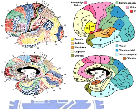
(Graphic source : http://spot.colorado.edu/ dubin/talks/brodmann/brodmann.html) Atlas of Talairach and Tournoux
In 1988, Talairach and Tournoux [28] introduced a stereotaxic atlas of the human brain based on dissection of an 60-year-old French female’s brain. They defined a standard co-ordinate system on this brain by making two points, the anterior commissure(AC) and pos-terior commissure(PC), lie on a straight horizontal line. Since AC and PC are both lie on midsagittal plane, the coordinate system is completely defined by requiring this plane to be vertical. Distances in Talairach coordinates are measured from the AC as origin. Talairach coordinate system approximately labels the Brodmann area based on visual inspection. In
other words, the location of brain structures in Talairach coordinate can be described ac-cording to the related Brodmann area. Fig 1.2 shows four slices of verticofrontal sections in Talairach atlas.
However, there are still some disadvantages of Talairach coordinate atlas. First, the brain examined for atlas creation was a 60-year-old French woman with a smaller than av-erage cranium cannot be a good representative of human brain. Additionally, the assump-tion of perfectly symmetry in Talairach brain seems irraassump-tional.Nonetheless, the Talairach atlas is still an invaluable tool in modern neuronimaging. It paved the way for subsequently brain atlas studies including the MNI atlas from the Montreal Neurological Institute.
MNI305
In 1994, in Montreal Neurological Institute (MNI), Evans et al. [9] constructed a population-based atlas which can represent the most people’s brain. The MNI created a MRI brain template called MNI305 which was based on averaging 305 normal subjects. The process of MNI305 construction consisted of two stages. First, 241 brain images were registered to Talairach coordinates and averaged to become the first-pass image. The registration was achieved by aligning several manually-specified landmarks of 241 brain images together by 9 parameters linear transformation. In the second stage, 305 normal MRI scans were linear normalized to the first-pass image as the same procedure in the first stage. Their average was computed to obtain the MNI305 template, which is the first template constructed by MNI. Fig. 1.3(a) shows the three different views of the MNI305 template.
ICBM152 and ICBM452
In 2001, the International Consortium for Brain Mapping (ICBM) used 152 normal subject MR scans to construct a template, called ICBM152 [21]. The 152 normal brains
1.1 Background 7
Figure 1.2: Talairach atlas. Talairach atlas of the human brain was introduced in 1988 by Talairach and Tournoux [28]. They defined a standard coordinate system based on dissec-tion of an 60-year-old French female’s brain. The Talairach atlas of anatomy constructed initially for stereotactic and functional neurosurgery is also used in human brain mapping, neuroradiology, medical image analysis, and neuroscience education. This figure shows four slices of verticofrontal sections in Talairach atlas.
(Graphic source : http://homepages.nyu.edu/ ef725/amygdala.html)
were registered to the MNI305 template using nine-parameter affine-transformation and averaged. These images were acquired at a higher resolution than the original 305 data of MNI305 due to advances in imaging technology. The ICBM152 template has been in-corporated into several widely used functional images analysis software packages, such as SPM, AFNI and FSL. Fig. 1.3(b) shows the three different views of the ICBM152 template.
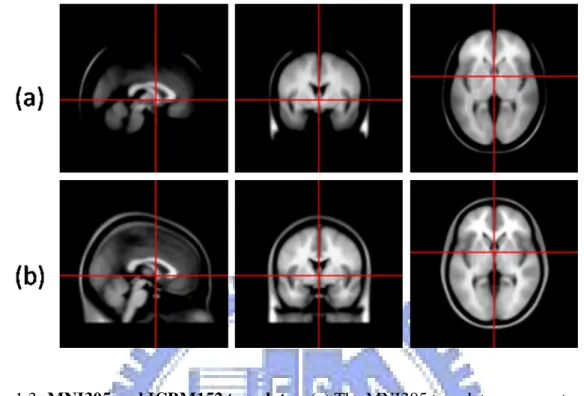
Afterward the ICBM created the ICBM452 template, which is a averaged of T1-weighted MRIs of normal young adult brains. The space the atlas is in is not based on any single
Figure 1.3: MNI305 and ICBM152 templates. (a) The MNI305 template was constructed by Montreal Neurological Institute (MNI) based on averaging 305 normal subjects. (b) The ICBM152 template was constructed by the International Consortium for Brain Mapping (ICBM) used 152 normal subject MR scans. These images were acquired at a higher res-olution than the original 305 data of MNI305. ICBM152 template has been incorporated into several widely used functional images analysis software packages.
(Graphic source : http://www.bic.mni.mcgill.ca/cgi/icbm view/)
subject, instead, an average space constructed from the average position, orientation, scale, and shear from all the individual subjects. ICBM452 is not yet widely used.
1.2
Procedure of Template Construction
There are various methods of template construction. We roughly divide these methods into two categories, manual procedures and automatic procedures. Intuitionally, manual procedures include manual landmark selection in template construction process contrary to automatic procedures. For example, MNI305 construction is a manual procedure. It
1.2 Procedure of Template Construction 9
involved affine registration which achieved by aligning several manually-specified land-marks.
Nowadays, with the progress of MR imaging and registration technique, fully comput-erized registration has outstanding performance. Therefore, several automatic methods of template construction have been developed. In the following paragraph, we will give a brief introduction to various studies about template construction.
Japanese Template
In 2003, Sato, Yaki, Fukuda, and Kawashima [23] collected 1547 normal and right-handed Japanese subjects including 772 men and 775 women between the ages of 16 and 79 years. In order to evaluate age-related structural changes of cerebral hemispheres, they divided subjects into 10 groups according to age and sex. The construction contained two stages. First, an brain of each group, which has the least deviation in brain shape with respect to the database , was selected as the reference subject in the group. All selected brains were spatially normalized to Talairach space using global scaling model. In second step, all brains in a group were normalized to the selected reference brain. These transfor-mation matrices defined the average size and shape of the brains. Then, the reference brain transformed to the average shape and size in this group by this transformation. Finally, the transformed brain was determined as reference (standard) brain of this age-sex group.
Korea Template
In 2005, 78 normal right-handed volunteers, including 49 males and 29 females, were recruited be Lee et al. [17] for the template construction. They were divided into 4 groups according to their genders (female and male) and ages (young and elderly). Two optimal
target brain of the templates for gender group were selected by manual method. They de-fined anterior commissure, posterior commissure, verticofrontal, and mid-sagittal planes by experts. The candidates of target brain in each group was determined by calculation of difference between these features. Subsequently, final selection of the target brains was conducted by experts manually. All brain images were normalized to the target brains of their gender group to form the four templates.
Human Cerebellum Template
Diedrichsen J. et al. [8] adopted an automatic template construction procedure to present a new high-resolution atlas template of the human, cerebellum and brainstem, in 2006. They claimed that the atlas is spatially unbiased, that is, the location of each structure is the expected location of that structure across individuals in MNI space. For any particu-lar structure i in the template should be equal to the average, or expected, location of that structure across all individuals n:
E(yi(n)) = zi, ∀i ∈ brainarea.
They used Colin27 brain as the reference brain to generate the unbiased cerebellun tem-plate. Each individual images were averaged in the space defined by Colin27, then the av-erage image applied the avav-erage deformation field to conduct the unbiased space.Compared to the normalization to the MNI whole-brain template, their method significantly improves the alignment of individual fissures, reducing their spatial spread by 60%, and improves the overlap of the deep cerebellar nuclei.
Neonatal Template
In 2007, Kazemi et al. [15] created a neonatal atlas template of newborns by an au-tomatic procedure. Their procedure shares some of the techniques used in the approach
1.3 Thesis Scope 11
presented by Diedrichsen J. et al. [8]. First, all images were affine registered to the refer-ence image, which is an arbitrary individual of brain images. The images resulting from the affine alignment are normalized to the reference image using nonlinear registration and resulted a average deformation field. Then the deformation field was applied to every brain images after nonlinear registered to the reference brain. Finally, the average brain template is calculated by averaging all transformed images. They repeated above process twice by replacing the reference image by the first pass template in order to minimizing the influence of the reference image.
They evaluated their template by anatomical local variation and amount of local de-formations of brain tissue with adult and pediatric templates. It was shown that using the neonatal template results in better performance as indicated by reduction of deviation of anatomical equivalent structures.
1.3
Thesis Scope
In this thesis, we provide an automatic procedure of MRI brain template construction. This non-manual and automatic process provides a convenient and efficient method to gen-erate a study-specific template without artifact. The intuition of constructing a template is simply averaging all brain volumes and resulting the average brain to be the template. Nev-ertheless, due to the different brain size, orientation and structure organization, the average image is inevitably too blurred to provide any information. Therefore, a common reference space must be defined so as to transform all brain images to this space before averaging.
Determination of the common reference space, however, is still an issue. We could use the MNI305 or ICBM152 templates, the widely-used templates, as our reference brain forthrightly. But because of Asian brain recruited in our study and the inter-ethnic
dif-ference of brain structure [35], we replace these widely-used templates with a optimal reference image within our brain database. After selection of reference image, called rep-resentative brain, we adopt the argument, introduced by Diedrichsen J. et al. [8], to create an unbiased space. Finally, all images are transformed to this unbiased space and averaged to result the template.
Furthermore, in order to quantitatively evaluate the generated template in comparison with ICBM152, we perform some evaluation experiments. Evaluations include study of amount of local deformations of brain tissues and the registration accuracy. On the other hand, we use the same evaluation method to verify the performance of the study specific template for both genders.
Except construction of brain template, we also provide generation of three different tis-sue templates including gray matter(GM), white matter(WM) and cerebral spinal fluid(CSF). All images are segmented in advance and then transformed to template space resulting the tissue templates.
In order to obtain the information of Talairach coordinates, we also provide a tool to derive the Talairach coordinates from our template space.
1.4
Thesis Organization
In the following chapters, we will present our algorithms, experiment results, discussion and conclusion. In chapter 2, we bring up our idea of automatic procedure of template construction. Because we try to verify the constructed templates, in chapter 3, we make a description of the template evaluation metrics. In chapter 4, we show all the experiment results. Then we have a discussion about the experiment results in chapter 5. Finally, in chapter 6, we make a conclusion.
Chapter 2
2.1
Introduction
The process of automatically constructing a spatially unbiased template can bedescribed in followingsteps, which is depicted in Fig. 2.1.
1. Nonuniformity correction
2. Selection of representative brain
3. Determination of unbiased stereotaxic space
4. Transformation and averaging
First, we use Non-parametric Non-uniform intensity Normalization (N3) [26] tech-nique, provided by Montreal Neurological Institute, to correct the nonuniformity of image. In the following steps, we use the corrected images to be processed. Second, because every brain images should be registered to a stereotaxic space before calculating the unbiased space, a reference brain is needed. We choose a brain volume, which is one subject of the image set and has the minimum variation of deformation magnitude to the other subjects, as the representative brain. Then we will define the unbiased space based on this repre-sentative brain. Thirdly, we compute the unbiased space according to the reprerepre-sentative brain and all other brain images. Finally, we normalize all images to the unbiased space and average them to generate the brain template.
2.2 Nonuniformity Correction 15
Figure 2.1: Flow chart of template construction. This figure describes the processed flow chart of the template construction. First, nonuniformity correction is performed to acquire images with better qualities. Second, a representative brain is selected among the data set to serve as the reference volume. Thirdly, the unbiased space is determined based on the selected representative brain and all other images. Finally, all images are transformed to this unbiased space and averaged to become the brain template.
2.2
Nonuniformity Correction
An intensity artifact, which the signal intensity vary smoothly across an image, is often seen in MR images. Variously referred to radio frequency (RF) inhomogeneity, shading ar-tifact, or intensity non-uniformity, it is usually attributed to poor RF field uniformity. How-ever, the image nonuniformity may significantly degrade the performance of automatic segmentation and interfere in quantitative analysis. Therefore, the removal of intensity nonuniformity (“bias”) from MRI images is an essential prerequisite for the quantitative analysis of MRI brain volumes. Fig. 2.2 shows the nonuniformity of MR images of a sub-ject in our database.
Figure 2.2: Nonuniformity of MR images. This figure shows the nonuniformity of MR images of a subject. There are four different slices in axial view of an individual brain. We can see the nonuniformity appeared, which the posterior white matter (in yellow region) is lighter than the anterior white matter.
devised in order to correct this intensity nonuniformity without requiring supervision. With-out anatomy model assumptions, an iterative approach is employed to estimate both the multiplicative bias field and the distribution of the true tissue intensity in N3 method. It models the low-frequency spatial variations in the data to maximize high-frequency infor-mation in the intensity histogram of the corrected volume. The N3 algorithm was demon-strated a high degree of stability [2], represents an elaboration of tissue signal analysis. Also N3 substantially improve the accuracy of anatomical analysis techniques such as tis-sue classification, cortical surface extraction [26] and grey matter segmentation for voxel-based morphometry [1]. An executable version of the N3 algorithm was provided by Dr. A. C. Evans at the Montreal Neurological Institute, and program default values were used for all run-time parameters.
2.3
Image Registration
Registration of structural brain images typically include affine transformation and non-linear deformation. In general, affine transformation, or called global normalization, is composed of zero or more linear transformations, including translation, rotation, scaling and shearing. Further, nonlinear deformation is used to match the subject to the target
im-2.3 Image Registration 17
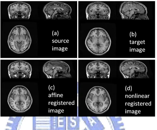
Figure 2.3: Affine registration and nonlinear registration. This figure shows the affine registration and nonlinear registration results. (a) This is the source image which is nor-malized to the target image. (b) This is the target image. We can tell the different brain size and shape between the source and the target. (c) The affine registered image of the source image is presented. The source image now is roughly registered to the target with the brain size. (d) The nonlinear registered image of the source image is showed. We can see the anatomical structure of the source brain is now registered to the target image, especially the corpus callosum region.
age on a regional level. The registration method adopted in this study is proposed by Liu et al. [18]. In their study, simulation data were used for validations and experiment results showed that the proposed registration approaches can efficiently register brain images with high accuracy compared to other algorithms, such as SPM2, AIR5 and ART. Fig. 2.3 shows the affine registration and nonlinear registration results of a subject in our database.
In image registration, two images are performed by serious deformations in order to make one image identical to the other. The result is stored in a deformation field, a vector field which records the magnitude and direction required to deform a point in the source
image to the appropriate point in the target image. The deformation function is
xT = xS+ dST(xS) (2.1)
, which xT is a point in the target image, xSis a point in the source image and dST(xS) is
the deformation vector of the point x.
2.4
Selection of Representative Brain
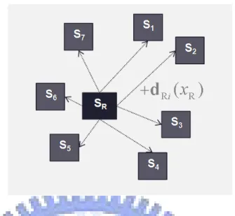
Because every brain images should be registered to a stereotaxic space before calculat-ing the unbiased space, a reference brain is needed [16]. There are several choices to select a reference volume such as the MNI305 template and the ICBM152 template. However, these different ethnic templates may cause large deformation while registering Taiwanese subject to them. Large deformation often conduct inaccuracy or instability of registration. Thus, we choose a brain volume, which is one subject of the image set and has the mini-mum variation of deformation magnitude to the other subjects, as the representative brain. In other words, the representative brain is defined to be the brain that is closer to all the brains than others. The definition of representative brain is as follows:
R = arg min
i {var(kdij(xi)k))|, ∀j 6= i, xi ∈ brain area, (2.2)
where dij(xi) is the deformation vector from subject i to subject j at position xiin the space
of subject i. The subject which has the minimum cost function, variation of deformation magnitude, with all the other subjects is chose as representative brain R. We describe this idea in Fig. 2.4.
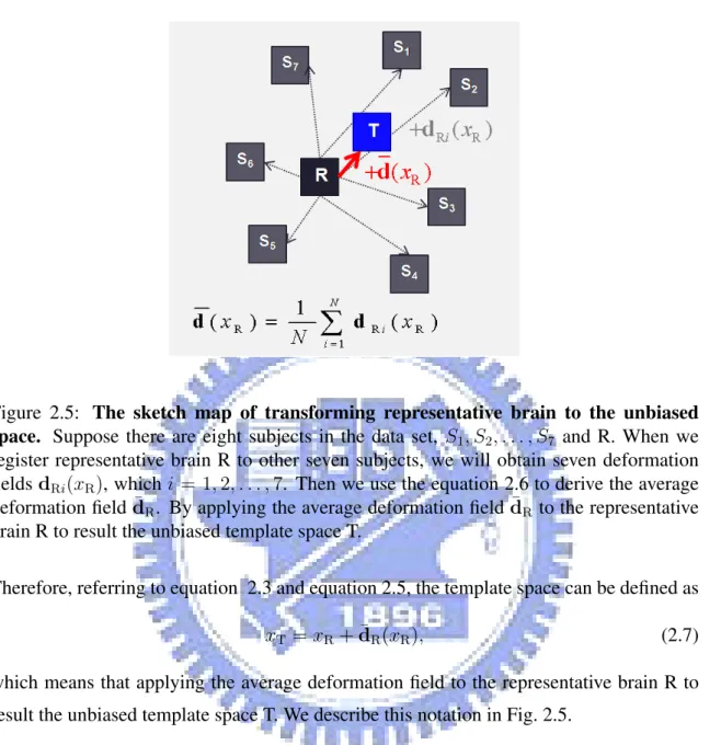
2.5
Determination of Unbiased Stereotaxic Space
Our goal is to create an unbiased space, the template, in which the structure location at the template denoted as xT should be equal to the expected location of that structure
loca-2.5 Determination of Unbiased Stereotaxic Space 19
Figure 2.4: The sketch map of selection of the representative brain. Suppose there are eight subjects in the data set, S1, S2, . . . , S7 and SR. When we register SRto other seven
subjects, we will obtain seven deformation fields dRi(xR), which i = 1, 2, . . . , 7. SRwill be
the selected representative brain if it has the minimum value of var(kdRi(xR)k) compared
with other subjects.
tion at subject i, denoted as xi, across all individuals N (a similar argument in Diedrichsen
J. et al. [8]) [12] [14]:
xT = E{xi}, (2.3)
where i = 1, 2, . . . N . That is, the expected deformation vector between xT and xi is zero.
However, we can regist representative brain R to subject i to get the deformation field. Referring to equation 2.1, dRi(xR) is the deformation vector from representative brain R
to subject i at position xR. Thus,
xi = xR+ dRi(xR), (2.4)
which xR+ dRi(xR) is the location in the space of subject i. Trivially,
E{xi} = E{xR+ dRi(xR)} = xR+ ¯dR(xR), (2.5)
where dRis the average deformation field which calculated by
¯ dR(xR) = 1 N N X i=1 dR(xR). (2.6)
Figure 2.5: The sketch map of transforming representative brain to the unbiased space. Suppose there are eight subjects in the data set, S1, S2, . . . , S7 and R. When we
register representative brain R to other seven subjects, we will obtain seven deformation fields dRi(xR), which i = 1, 2, . . . , 7. Then we use the equation 2.6 to derive the average
deformation field ¯dR. By applying the average deformation field ¯dR to the representative
brain R to result the unbiased template space T.
Therefore, referring to equation 2.3 and equation 2.5, the template space can be defined as xT = xR+ ¯dR(xR), (2.7)
which means that applying the average deformation field to the representative brain R to result the unbiased template space T. We describe this notation in Fig. 2.5.
The representative brain is registered to each nonuniformity-corrected image. We ob-tain each deformation field dRi(xR) and average them to become the average deformation
field ¯dR. It is notable that the deformation vectors, stored in the average deformation field,
record the vector required to deform points, called voxels, in representative brain to the appropriate voxels in unbiased space. This unbiased space is our template space.
However, due to the sub-voxel accuracy of the average deformation field ¯dR, the
2.5 Determination of Unbiased Stereotaxic Space 21
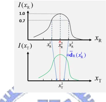
Figure 2.6: The sketch map of interpolating the mapping coordinate in the unbiased space. The intensity profile of the representative brain is shown as I(xR). When
compress-ing the profile of representative to become the profile of the template, the ideal profile of template is shown as I(xT) (green profile). x1R and x3R plus the average deformation
vec-tors, ¯dR(x1
R)and ¯dR(x3R)to the sub-voxel position in unbiased space. However, the intensity
of x2T must not be derived by simply averaging the intensity of I(x1R) and I(x2R), which is 0.7. Instead of averaging the intensity, it should calculate the corresponding position in the xR, which is x2Rin this case, and finally derive the intensity of x
2
T, which is 1.0.
Suppose the image signal is a one dimensional signal, and the intensity profile of the repre-sentative brain is shown as I(xR). The point x1R and x3Rare deformed to sub-point position
in template space. In that case, the intensity of point x2
T in template space is not to know.
However, the intensity of x2Tmust not be derived by simply averaging the intensity of I(x1R) and I(x2R). Instead of averaging the intensity, it should calculate the corresponding position in the xR, which is x2Rin this case, and finally derive the intensity of x2T.
In this thesis, we propose a interpolation method to calculate the corresponding position in the xR. A voxel xTin the unbiased space, or said template space, is corresponding to xTR
in the representative space. Then the intensity of xT is I(xT) is defined as:
We interpolate the xTR position by the following equation : xTR = 1 PMT i=1wi MT X i=1 wiyi, yi ∈ neighbor of xT. (2.9)
In equation 2.9, w is the Gaussian weight which defined as f (x, y, z) = Ae−( (x−x0)2 2σ2x )−( (y−y0)2 2σ2y )−( (z−z0)2 2σ2z ),
which f (x, y, z) is the Gaussian value according the center at (x0, y0, z0), A is the
Gaus-sian amplitude, and σx, σy, σz are the the x, y and z spreads of the blob. Therefore, by
equation 2.8 and equation 2.9, we finally derive the intensity of all voxels in the unbiased space.
2.6
Average Template in Unbiased Space
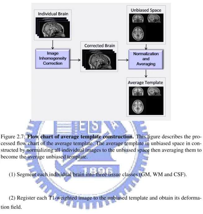
After we derive the unbiased space, we normalize all MR T1-images, which have been corrected the intensity inhomogneity, to the unbiased space. Then we average them to become the average template. However, because this unbiased space is derived from the representative brain, the brain size and orientation of the generated template is significantly dependent on the representative brain. Suppose the representative brain is not located in the center of the MR image, then the brain template will not located in the center of the MR image. Fig. 2.7 describes the processed flow chart of the average template.
2.7
Brain Tissue Templates
Brain tissue could be classified into three different types, gray matter (GM), white mat-ter (WM) and cerebral spinal fluid (CSF). Inthe thesis, GM, WM and CSG tissue templates are generated by the following steps:
2.7 Brain Tissue Templates 23
Figure 2.7: Flow chart of average template construction. This figure describes the pro-cessed flow chart of the average template. The average template in unbiased space in con-structed by normalizing all individual images to the unbiased space then averaging them to become the average unbiased template.
(1) Segment each individual brain into three tissue classes (GM, WM and CSF).
(2) Register each T1-weighted image to the unbiased template and obtain its deforma-tion field.
(3) Normalize every tissue segment of all individuals by their own deformation field in step 2.
(4) Average all these normalized tissue segments and finally form the templates of three tissue classes.
Figure 2.8: Flow chart of tissue templates construction. This figure describes the pro-cessed flow chart of the tissue templates. First, we segment each individual brain into GM, WM and CSF by FMRIB’s Automated Segmentation Tool (FAST). Then we register each T1-weighted image to the unbiased template and obtain its deformation field. After we obtain the deformation field, we normalize every tissue segment of each individual by ap-plying its own deformation field. Finally, the tissue templates are generated by averaging all these normalized tissue segments.
Segmentation are performed by FMRIB’s Automated Segmentation Tool (FAST) [27] [13]. The tissue templates procedure is shown in Fig. 2.8.
2.8
Mapping to Talairach Coordinate System
Talairach coordinate system is widely used as a reference with Brodmann cytoarchi-tectonic areas and other structural and functional labels. Therefore, we should provide the mapping method between our template and the Talairach coordinate system. In other words, we intend to create a transformation to apply to the coordinates from the our brain template, to give matching coordinates in the TB. However, because there is no MRI scan
2.8 Mapping to Talairach Coordinate System 25
for the Talairach brain, we are incapable of using computerized registration to simply trans-form our template to Talairach brain.
Since there are already tools that can transform a coordinate in the MNI template space to the Talairach space [6], we use MNI template as the bridge to Talairach space by trans-forming the coordinate in our template to MNI template first. Thus, the mapping coordi-nate in Talairach space will be calculated by the second transformation from MNI305 to Talairach space.
To implement the method illustrated above is registering our template to the MNI tem-plate to obtain the deformation field. This deformation field stores the appropriate mapping coordinate in MNI template space of every voxel in our template. Then we derive Talairach coordinates from mni2tal script (http://www.mrc-cbu.cam.ac.uk/ ˜matthew/abstracts/ MNI-Tal/mnital.html) , a tool commonly used to map MNI coordinates to Talairach coordi-nates [3]. Also we register MNI template to our template and transform the coordinate in Talairach space to out template space.
Chapter 3
3.1
Introduction
In order to quantitatively evaluate the constructed template in comparison with the dif-ferent templates, including the widely-used template nowadays, we use two metrics in our evaluation procedure. The template serves as the reference space for all images transform-ing to it. Thus, the template, which provides the better registration accuracy for all images of the study group, can be defined as the better template. Therefore, we use two metrics to verify the performance that our template improves. The two factors are:
1. Nonlinear deformation field between subjects and templates
2. Similarity between registered subjects and templates
3.2
Nonlinear Deformation Field between Subjects and
Tem-plates
3.2.1
Magnitude of Deformation Field
A good template should cause distortion of deformation as small as possible because large deformation may raise registration inaccuracy. Therefore, magnitude of deformation field is a good way to measure the distortion. This evaluation aims to study the amount of local nonlinear deformation needed to perform the normalization. A small total amount of these local changes indicates a small overall difference in shape between images and template [15].
3.2 Nonlinear Deformation Field between Subjects and Templates 29
field can be calculated as the distance between corresponding points in the template and the original image after affine transformation. We average the magnitude of nonlinear deformation vectors for overall voxels of each individual brain. The magnitude of nonlinear deformation field is defined as average distance (AD):
AD = 1 M N N X i=1 M X x=1
dTi(xT), ∀xT∈ brain area of the template, (3.1)
which M is the total number of voxels in brain area.
However, in order to examine the distribution of average nonlinear deformation mag-nitude, we also display the topography of deformation. While calculating the deformation field from the template to individual brains, magnitude of nonlinear deformation field on same voxel of every brain were recorded. Then we calculate the mean of the recorded values for every voxel. Thus, we can investigate the distribution of nonlinear deformation magnitude.
3.2.2
Variance of Deformation Field
By observing the variance of nonlinear deformation field, we can know the anatomically regional variability of the difference between the template and individual brains. However, a good template should cause not only small distortion magnitude of deformation but also small distortion variance. When the variance of nonlinear deformation field is zero, this template is called unbiased to the individual brains. For calculating the variance, when we normalize subjects to the template, the deformation magnitude of each voxel is recorded. We calculate the variance of all magnitudes in the same voxel of all brain images. Finally, we obtain the topography of variance of nonlinear deformation field.
3.3
Similarity between Registered Subjects and Templates
The deformation magnitude only provides the amount of normalization distortion. How-ever, the less distortion can not imply the higher registration accuracy. That is to say, if we normalize a brain to a template which barely provides any information, the deformation is small but the result of registration is poor. For this reason, we aim to study the similarity between the template and the images after normalization for the anatomical evaluation. We anticipate that when using the better template, the warped brain images are more similar to the template. Here, we intend to compare the accuracy of normalization of all images of a study-specific group using different templates.
Each of the individual brain were warped to different templates and compared their spatial likeness against different templates. However, the correlation ratio, introduced by Roche, A. et al. in 1998 [24], provides the similarity measure for MR images. We calculate the average of correlation ratio between the template and each normalized images. The larger correlation ratio is, the similar the template and images are, i. e. the similar are the two, provided the normalization result is reasonable.
Chapter 4
4.1
Materials
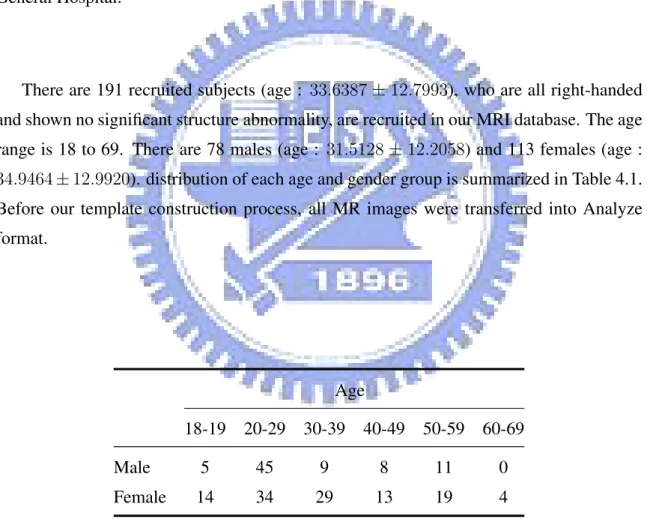
The database was constructed with normal brains of different generations and genders. The magnetic resonance images were acquired on a 1.5 Tesla GE MR scanner, using 3D-FSPGR pulse sequence (TR = 8.67 ms, TE = 1.86 ms, TI = 400 ms, NEX = 1, flip angle = 15◦, bandwidth = 15.63 kHz, matrix size = 256 × 256 × 124, voxel size = 1.02 × 1.02 × 1.5). All MR scans were collected by Integrated Brain Research Unit (IBRU) of Taipei Veterans General Hospital.
There are 191 recruited subjects (age : 33.6387 ± 12.7993), who are all right-handed and shown no significant structure abnormality, are recruited in our MRI database. The age range is 18 to 69. There are 78 males (age : 31.5128 ± 12.2058) and 113 females (age : 34.9464 ± 12.9920). distribution of each age and gender group is summarized in Table 4.1. Before our template construction process, all MR images were transferred into Analyze format.
Age
18-19 20-29 30-39 40-49 50-59 60-69 Male 5 45 9 8 11 0 Female 14 34 29 13 19 4 Table 4.1: Number of subjects in our database.
4.2 Construction of Brain Templates 33
4.2
Construction of Brain Templates
4.2.1
Nonuniformity Correction
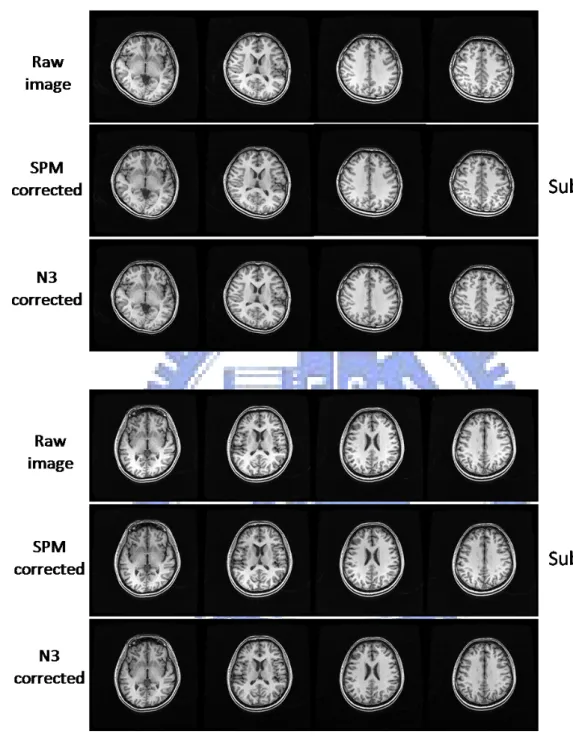
We used Non-parametric Non-uniform intensity Normalization (N3) [26] tool to cor-rect the nonuniformity of MR images in order to obtain the higher quality of images. An executable version of the N3 algorithm was provided by Dr. A. C. Evans at the Montreal Neurological Institute, and program default values were used for all run-time parameters. On the other hand, we used the nonuniformity correction tool provided by SPM2 to com-pare the performance with N3.
We examined the MR images which corrected by N3 tool and found N3 provide a high degree of stability and substantially improve the quality of the MR images. Here we ran-domly selected four subjects to show the results of nonuniformity correction in Fi. 4.1 and Fig. 4.2. In the subject1 and subject2, the nonuniformity of raw images are more evident than that in subject3 and subject4. However, the overall performance of N3 is better than SPM.
4.2.2
Selection of Representative Brain
Large deformation often conduct inaccuracy or instability of registration. Thus, we choose a brain volume, which is one subject of the image set and has the minimum varia-tion of deformavaria-tion magnitude to the other subjects, as the representative brain. Refering to equation 2.2, the var(kdij(xi)k, ∀j 6= i must be calculated. Take notice of kdij(xi)k is
not identical to kdji(xj)k. In other words, if we try to determine the representative brain
within N subjects, we need to do the all-paired registration N2 times.
Figure 4.1: Results of nonuniformity correction using SPM and N3 for subject1 and subject2. For each subject, we showed four slices the raw image, nonuniformity correction using SPM and nonuniformity correction using N3 in three raws. We can see the nonuni-formity appeared in raw the image, where the posterior region of white matter is lighter than the anterior white matter. The nonuniformity has been evidently improved after N3-correction comparing with SPM.
4.2 Construction of Brain Templates 35
Figure 4.2: Results of nonuniformity correction using SPM and N3 for subject3 and subject4. For each subject, we showed four slices the raw image, nonuniformity correction using SPM and nonuniformity correction using N3 in three raws. We can see the nonuni-formity appeared in raw the image, where the posterior region of white matter is lighter than the anterior white matter. The nonuniformity has been improved after N3-correction comparing with SPM.
which age range is 18 to 35 years old (25.5339 ± 5.0728), as the candidates of the rep-resentative brain. There are total 126 subjects, including 57 males and 69 females. Ta-ble 4.2 shows the distribution of each age and gender group. The value of the cost function, var(kdij(xi)k, ∀j 6= i, is 78.3439 ± 160.2550 mm/voxel. Table 4.3 lists the mean value of
the cost function in each group.
A 23 years old female is selected as the representative brain within 126 subjects. It’s value of cost function is 6.8458, which is the minimum value of all 126 subjects. The MR image of the representative brain is shown in Fig. 4.3.
Age
18-19 20-29 30-35 Male 5 45 7 Female 14 34 21
Table 4.2: Number of subjects of candidates for representative brain.
Age
18-19 20-29 30-35 Mean 74.1643 77.1644 84.5079 Std. 101.8881 145.4536 225.3896
Table 4.3: Mean and standard deviation of cost function for selection of representative brain.
4.2 Construction of Brain Templates 37
Figure 4.3: The selected representative brain. The selected representative brain, a 23 years old female’s brain, from 126 subjects with age range from 18 to 35 years old.
4.2.3
Determination of Unbiased Stereotaxic Space
After selecting the representative brain, 191 normal subjects were taken to calculate the unbiased space. Age range is from 18 to 69 years old (33.6387 ± 12.7993). The representative brain was normalized to other 190 individual brains. We obtained the aver-age deformation field by averaging all nonlinear deformation fields with respect to all 190 brains. Then we applied the average deformation field to the representative brain to derive the unbiased space. In this step, we utilized proposed interpolation method. Fig. 4.4 shows the representative brain and the derived unbiased space.
4.2.4
The Unbiased Average Templates
After we derived the unbiased space, we normalized all 191 MR T1-images in our database to the unbiased space. Then we averaged them to become the 191 average tem-plate. Otherwise, we segmented all 191 MR images into gray matter (GM), white matter (WM) and cerebral spinal fluid (CSF) and normalized them to this unbiased space accord-ing to their own deformation fields. GM, WM and CSF templates were also created. All these templates are shown in Fig. 4.5.
Prime Templat
We also constructed a brain template for the prime of life (Fig. 4.6(b)). There are 126 subjects, including 57 males and 69 female, which age range is 18 to 35 years old (25.5339 ± 5.0728).Number of subjects for construction is shown in Table 4.4. The repre-sentative brain for prime group is a 23-year-old female brain, which is identical to whole subject group.
4.2 Construction of Brain Templates 39
Figure 4.4: The representative brain and the unbiased space. (a) The representaive brain. (b) The derived unbiased space from (a) and all other 190 subjects in MRI brain database.
Gender templates
We constructed brain template for both gender groups (Fig. 4.6(c)(d)). There are 57 males (age : 24.7895 ± 4.0565) and 69 female (age : 26.2754 ± 5.7596), which age range is 18 to 35 years old in our database.Number of subjects for construction is shown in Ta-ble 4.4. The representative brain for male group is a 24-year-old male brain. Additionally, the representative brain for female group is the same brain as for whole group, a 23-year-old female brain.
Age
18-19 20-29 30-35 Male 5 45 7 Female 14 34 21
Table 4.4: Number of subjects for construction of prime template and gender template.
Age Templates
We constructed brain templates for each age groups, including 10 to 19, 20 to 29, 30 to 39, 40 to 49, 50 to 59 (Fig. 4.7). Table 4.1 shows number of data. However, because there are only 4 subjects that age range from 60 to 69 years old, there is no significance to build the template for this age group.
4.2 Construction of Brain Templates 41
Figure 4.5: The 191 average template and the tissue templates. (a) The average tem-plate constructed from 191 subjects. (b) The GM temtem-plate, (b) WM temtem-plate and (c) CSF template.
Figure 4.6: The 191 average template, the prime template and the gender templates. (a) The average template constructed from 191 subjects. (b) The prime template con-structed from 126 subjects, which age range is from 18 to 35 years old. (b) The male template constructed from 57 male subjects (age : 24.7895 ± 4.0565). (c) The female tem-plate constructed from 69 female subjects (age : 26.2754 ± 5.7596). We affine registered these four templates together for the convenient and fair comparison.
4.2 Construction of Brain Templates 43
Figure 4.7: The brain templates for each age groups. (a) The template was constructed by subjects which from age 10 to 20. (b) The template was constructed by subjects which from age 20 to 30. (c) The template was constructed by subjects which from age 30 to 40. (d) The template was constructed by subjects which from age 40 to 50. (e) The template was constructed by subjects which from age 50 to 60. We affine registered these five templates together for the convenient and fair comparison.
4.3
Evaluation of Brain Templates
4.3.1
Nonlinear Deformation Field
When we normalized a MR brain images to a space, or a space, we obtained a deforma-tion field. This evaluadeforma-tion aims to study the amount of local nonlinear deformadeforma-tion needed to perform the normalization.
Unbiased template v.s. ICBM152
We normalized all subjects, 191 subjects in our database, to the average template con-structed from these 191 subjects and the ICBM152 template. The average magnitude of local nonlinear deformation of all subjects was listed in Table 4.5. We displayed the dis-tribution of regional nonlinear deformation magnitude in brain region of each template (Fig. 4.8). While calculating the deformation field from each template to 191 individ-ual brains, magnitude of nonlinear deformation field on same voxel of every brain were recorded. Then we calculated the mean of the recorded values for every voxel. Finally, a brain volume that its voxel value represents mean value of magnitude on same voxel was generated. Here we took the unbiased space, the unbiased average template generated by 191 subjects and ICBM152 to observe the regional magnitude of nonlinear deformation.
Otherwise, we also calculated the variance of deformation of these two templates (Fig. 4.9). We normalized all subjects, 191 subjects in our database, to two different templates, the average template created from these 191 subjects and the ICBM152 template. The defor-mation vector in each voxel was recorded in the 191 defordefor-mation field. Then we calculated the variance of the recorded values for every voxel. Finally, a brain volume that its voxel value represents the variance of deformation vector on same voxel was generated.
4.3 Evaluation of Brain Templates 45
Template
Unbiased average template ICBM152 AD 1.7556 2.4572 Var. 7.6677 8.4774
Table 4.5: The mean and variance magnitude of nonlinear deformation comparing Unbiased template v.s. ICBM152. The mean and variance magnitude of nonlinear de-formation from 191 subjects to both the unbiased template created from these 191 subjects and ICBM152 template were listed.
In order to evaluate the unbiased template with ICBM152 disinterestedly, we used 65 elder subjects, age range is from 36 to 69, in our database as the testing data. We normal-ized these 65 subjects to the prime-age template, which was constructed by 126 prime-age subjects, age range is from 18 to 35. In this case, the prime-age unbiased template was not consisted of any testing data. In the other hand, we also normalized these 65 subjects to ICBM152. We calculated the nonlinear deformation magnitude and variance from all 65 subjects to both templates. The mean of magnitude and variance is listed in Table. 4.6. We displayed the distribution of regional nonlinear deformation magnitude in brain region of each template (Fig. 4.10) and nonlinear deformation variance (Fig. 4.11).
Template
Prime-age unbiased template ICBM152 AD 0.8215 1.9907 Var. 4.1604 9.9779
Table 4.6: The mean and variance magnitude of nonlinear deformation comparing prime-age unbiased template v.s. ICBM152. The mean and variance magnitude of non-linear deformation from 65 elder subjects to both the prime-age unbiased template created from prime-age 126 subjects and ICBM152 template were listed.
Figure 4.8: The distribution of nonlinear deformation magnitude to Unbiased Tem-plate and ICBM152 temTem-plate. We normalized 191 brain images to both the unbiased template constructed by these 191 subjects and ICBM152 template. We averaged the mag-nitude of nonlinear deformation on the same voxel of each brain. Then, the brain volume that its voxel value represents the mean of the nonlinear deformation was formed. The left figure showed the distribution on slices in axial view.
4.3 Evaluation of Brain Templates 47
Figure 4.9: The distribution of nonlinear deformation variance to Unbiased Template and ICBM152 template. We normalized 191 brain images to both the unbiased template constructed by these 191 subjects and ICBM152 template. We calculated the variance of nonlinear deformation on the same voxel of each brain. Then, the brain volume that its voxel value represents the variance of the nonlinear deformation was formed. The left figure showed the distribution on slices in axial view.
Figure 4.10: Nonlinear deformation magnitude of 65 elder subjects to prime-age unbi-ased template and ICBM152 template. We normalized 65 elder brain images to both the prime-age unbiased template constructed by 126 prime-age subjects and ICBM152 tem-plate. We averaged the magnitude of nonlinear deformation on the same voxel of each brain. Then, the brain volume that its voxel value represents the mean of the nonlinear deformation was formed. The left figure showed the distribution on slices in axial view.
4.3 Evaluation of Brain Templates 49
Figure 4.11: Nonlinear deformation variance of 65 elder subjects to prime-age unbi-ased template and ICBM152 template. We normalized 65 elder brain images to both the prime-age unbiased template constructed by 126 prime-age subjects and ICBM152 tem-plate. We calculated the variance of nonlinear deformation on the same voxel of each brain. Then, the brain volume that its voxel value represents the variance of the nonlinear deformation was formed. The left figure showed the distribution on slices in axial view.
Bisexual template v.s. gender template
We used proposed method in this thesis to construct the bisexual template, including 126 male and female subjects, and two gender templates, the male template constructed by 57 males and the female template constructed by 69 females. The subject number is in Table 4.7.
Template
Bisexual template Male template Female template Subjects 126 57 69
Age 25.5339 ± 5.0728 24.7895 ± 4.0565 26.2754 ± 5.7596
Table 4.7: Number of subjects for construction of bisexual template and gender templates.
We normalized 57 male subject brains to both the bisexual template and the male tem-plate and obtained the nonlinear deformation field. Also we normalized 69 female subject brains to both the bisexual template and the female template and obtained the nonlinear de-formation field. The mean magnitude and variance of local nonlinear dede-formation of male and female subjects was listed in Table 4.8 and Table 4.9.
We displayed the distribution of regional nonlinear deformation magnitude or variance in brain region of both the bisexual template and gender template (Fig. 4.12 to Fig. 4.15) . While calculating the deformation field from each template to different gender brains, magnitude or variance of nonlinear deformation field on same voxel of every brain were recorded. Then we calculated the mean or variance of the recorded values for every voxel. Finally, a brain volume that its voxel value represents mean value of magnitude on same voxel was generated. Here we observed the distribution of nonlinear deformation magni-tude or variance of both the unbiased bisexual template and the male template. Similarly,
4.3 Evaluation of Brain Templates 51
Template
Bisexual template Male template Female template Male 0.8514 0.6574
-Female 0.9347 - 1.0088
Table 4.8: The average magnitude of nonlinear deformation comparing Bisexual tem-plate, Male temtem-plate, and Female template. The average magnitude of nonlinear de-formation from male or female subjects to both the unbiased template, created from both gender subjects, and their own gender template were listed.
Template
Bisexual template Male template Female template Male 0.7637 0.4824
-Female 0.8808 - 0.6527
Table 4.9: The variance of nonlinear deformation magnitude comparing Bisexual tem-plate, Male temtem-plate, and Female template. The variance of nonlinear deformation mag-nitude from male or female subjects to both the unbiased template, created from both gen-der subjects, and their own gengen-der template were listed.
we examined the distribution of nonlinear deformation magnitude or variance which were calculated from female subjects to the bisexual template and the female emplate.
4.3.2
Similarity between Registered Subjects and Templates
For the anatomical evaluation, we studied the similarity between the template and the images after normalization. We compared the accuracy of normalization of all images of a study-specific group using different templates.
Figure 4.12: The distribution of nonlinear deformation magnitude to the bisexual tem-plate and the male temtem-plate. We normalized 57 male subjects to both the the bisexual template and the male template. We averaged the magnitude of nonlinear deformation on the same voxel of each brain. Then, the brain volume that its voxel value represents the mean of the nonlinear deformation was formed. The left figure showed the distribution on slices in axial view.
4.3 Evaluation of Brain Templates 53
Figure 4.13: The distribution of nonlinear deformation variance to the bisexual tem-plate and the male temtem-plate. We normalized 57 male subjects to both the the bisexual template and the male template. We calculated the variance of nonlinear deformation on the same voxel of each brain. Then, the brain volume that its voxel value represents the variance of the nonlinear deformation was formed. The left figure showed the distribution on slices in axial view.
Figure 4.14: The distribution of nonlinear deformation magnitude to the bisexual tem-plate and the female temtem-plate. We normalized 69 female subjects to both the the bisexual template and the female template. We averaged the magnitude of nonlinear deformation on the same voxel of each brain. Then, the brain volume that its voxel value represents the mean of the nonlinear deformation was formed. The left figure showed the distribution on slices in axial view.
4.3 Evaluation of Brain Templates 55
Figure 4.15: The distribution of nonlinear deformation variance to the bisexual tem-plate and the female temtem-plate. We normalized 69 female subjects to both the the bisexual template and the female template. We calculated the variance of nonlinear deformation on the same voxel of each brain. Then, the brain volume that its voxel value represents the variance of the nonlinear deformation was formed. The left figure showed the distribution on slices in axial view.
![Figure 1.2: Talairach atlas. Talairach atlas of the human brain was introduced in 1988 by Talairach and Tournoux [28]](https://thumb-ap.123doks.com/thumbv2/9libinfo/8698694.199021/21.892.172.823.119.704/figure-talairach-atlas-talairach-atlas-introduced-talairach-tournoux.webp)