隱含波動度, 投資人情緒與市場指數之互動關係與策略應用

(1)

國立交通大學

管理科學系

博士論文

No. 054

隱含波動度, 投資人情緒與市場指數之

互動關係與策略應用

The Interaction and Strategy Application between

Implied Volatility, Investor Sentiment and Market Index

研究生：魏裕珍

指導教授：許和鈞教授

(2)

國立交通大學

管理科學系

博士論文

No. 054

隱含波動度, 投資人情緒與市場指數之

互動關係與策略應用

The Interaction and Strategy Application between

Implied Volatility, Investor Sentiment and Market Index

研究生：魏裕珍

研究指導委員會：謝國文教授

研究指導委員會：

鍾惠民教授

指導教授：許和鈞教授

(3)

隱含波動度, 投資人情緒與市場指數之

互動關係與策略應用

The Interaction and Strategy Application between

Implied Volatility, Investor Sentiment and Market Index

研究生：魏裕珍

Student：Yu-Chen Wei

指導教授：許和鈞

Advisor：Her-Jiun Sheu

國立交通大學

管理科學系

博士論文

A Dissertation

Submitted to Department of Management Science

College of Management

National Chiao Tung University

in Partial Fulfillment of the Requirements

for the Degree of

Doctor of Philosophy

in

Management

July 2010

Hsin-Chu, Taiwan, Republic of China

(4)

隱含波動度, 投資人情緒與市場指數之

互動關係與策略應用

研究生：魏裕珍

指導教授：許和鈞

國立交通大學管理科學系博士班

中文摘要

本文由行為財務學角度剖析隱含波動度、投資人情緒與市場指數之互動關係，並以臺灣證券市場資料構建波動度指數及投資人情緒指標之代理變數進行相關實證分析及策略應用。研究內容主要分為三個部分。第一部分應用門檻模型(Chan, 1993)檢測投資人情緒過度反應之門檻水準，並剖析不同市場狀況下，投資人情緒與市場報酬間之因果關係，實證結果顯示若未考慮市場狀態，投資人情緒指標與市場報酬之間存在雙向之因果關係，然而，當投資人情緒在極端高或低之區域時，對於市場報酬將具有指引效果。第二部分則應用門檻共整合模型(Hansen and Seo, 2002)探討波動度指數之資訊內涵與標的指數間之關聯性，實證結果顯示，當買權之隱含指數領先加權股價指數時，臺灣證券市場之參與者可應用此資訊做為投資組合調整之參考。第三部分進一步考量投資人情緒指標進行波動度預測，並應用至選擇權交易策略，比較結果顯示，若納入投資人情緒指標，模型之配適與預測績效將優於其他比較模型，特別是納入市場週轉率與市場恐慌指標代理變數-選擇權隱含波動度。綜而觀之，在探討波動度、投資人情緒與市場指數之互動關係時，應將投資人情緒可能存在的不對稱效果納入考量，未來的研究亦可進一步納入投資人情緒的不對稱效果進行波動度預測，並將研究結果實際應用至交易策略中。關鍵詞：隱含波動度、投資人情緒、波動度預測、門檻模型、因果、選擇權交易策略

(5)

The Interaction and Strategy Application between

Implied Volatility, Investor Sentiment and Market Index

Student：Yu-Chen Wei

Advisor：Her-Jiun Sheu

Department of Management Science

National Chiao Tung University

Abstract

This dissertation investigates the interaction among implied volatility, investor sentiment and market index from the behavioral finance point of view. The volatility measures and proxies of investor sentiment are constructed and the empirical results and strategy application are analyzed in the emerging Taiwan equity market.

There are three main parts in this study. In the first part, we apply a threshold model (Chan, 1993) to detect the extreme level of investors‟ sentiment econometrically and investigate the causal relationships between sentiment and returns under different market scenarios. The empirical results show that most of the sentiment measures exhibit a feedback relationship with returns while ignoring different market states. However, sentiment could be a leading indicator if the higher or lower levels of sentiments being distinguished. In the second part, the relationship between the information content implied by the options market-based volatility and the underlying stock index is analyzed through a threshold cointegration model (Hansen and Seo, 2002). Empirical findings show that investors participating in the Taiwan stock market could rebalance their equity portfolios while the implied index derived from the call options takes precedence over the market index. In the last part, an algorithm for effective options trading strategy based on volatility forecasts incorporating investor sentiment is proposed. The forecast evaluation supports the significant incremental explanatory power of investor sentiments in the fitting and forecasting of future volatility in relation to its adversarial multiple-factor model, especially the market turnover and the volatility index which is referred to as the investor fear gauge.

Overall, the asymmetric property of investor sentiment should be incorporated into the interactive analysis between volatility, sentiment and market index. Future research could further investigate the volatility forecasting incorporating the asymmetry of investor sentiment and apply the findings to the actual trading strategies.

Keywords: Implied volatility, Investor sentiment, Volatility forecasting, Threshold

(6)

致謝辭

執筆寫下致謝辭的此時，回想起求學生涯的點點滴滴，歷歷在目，心裡是溫暖而踏實的，求學之路峰迴路轉，我的人生與心境都有了不同的體驗，完成論文取得博士學位，是一個里程碑也是另一個開始，感謝這段旅程中陪伴與提攜我的家人、師長與朋友，也期許自己的人生旅程能學以致用，不忘飲水思源。感謝指導教授許和鈞博士，許多的因緣際會之下，有幸能成為老師的學生，老師的為人處事與治學嚴謹為我樹立了學習的典範，也感謝老師無私地與我分享研究資源，讓我能盡情地在研究領域努力嘗試，求有還要求好，未來我將持續投入研究與教學，希望能有更好的成果回饋老師的教誨之恩。感謝謝國文教授與鍾惠民教授，兩位老師一方面是我的研究指導委員會，一方面也都是我博士班求學過程的授課老師，謝國文老師課堂中一席｢今日的成果源自於兩年前的努力｣，讓我每當遇到瓶頸時總能心平靜氣的度過，也讓我稍遇順境時能更警惕自己努力不怠；鍾惠民老師不但在博士班授課過程給我許多研究觀念的啟發，也是我碩士班求學期間計量課程的老師，與鍾老師十年來的師生緣分，亦分外讓我珍惜。感謝我的口試委員沈中華教授與黎明淵教授，兩位老師百忙之中仍替學生著想，讓學生的口試能圓滿舉行，感謝沈中華老師鉅細靡遺地審閱學生的博士論文，提供學生修改建議，讓學生的論文更完整，也提供學生許多研究的想法，沈老師對於教學研究的熱情及教育產業的理念，展現了大師風範；感謝黎明淵教授對於學生論文中採用的研究方法，提出不同觀點的見解，並提供學生財務意涵之詮釋，黎老師在學術研究的卓越成果，值得學生學習。我的求學生涯中，還有許多老師讓我感銘在心。盧陽正老師是我在銘傳大學財金系就讀碩士班的指導教授，我有念頭攻讀博士學位，也是緣於盧老師指導的碩士論文得到國科會碩士論文獎，盧老師一路看著我從懵懂的大學畢業生，到如今為人妻為人母並完成博士學位，盧老師參與我許多人生轉折，飲水思源，我也希望在老師創造歷史的過程，能有所回饋；在我碩士班至博士班的求學生涯中，有幸能與林建甫教授、張倉耀教授、聶建中教授、陳達新教授與周冠男教授在研討會與學術聚餐中結緣，幾位老師在研究議題、研究方法與治學態度上，給予學生諸多建議與提攜；藉著研究計劃的參與，我有機會與陳振南教授與陳耀竹教授進行財務、資訊與傳播跨領域的研究，老師們雖然都身兼數職，但對研究始終抱持無限的熱情；幾位老師將是我研究生涯的學習典範與良師至寶。求學過程除了感謝師長們的提攜與鼓勵外，家人的支持更給予我無形的力量，讓我奮戰不懈。感謝我的母親古碧珠女士，他身兼母職與父職，是我人生低潮與失落時的避風港，讓我能蓄積能量勇往直前，感謝我的父親魏朝光先生，父親是我堅持理想的一盞明燈，雖然他在著作升等副教授的同一年辭世，但我能

(7)

取得博士學位，也算是完成父親的一個心願，感謝我的兩個弟弟君洪、君祐及弟妹欣淳，在我埋首書本的同時，替我陪伴與照顧母親。感謝老公羅德智，因為有他，讓我無後顧之憂地完成我的博士學位，感謝我的公婆羅亞察先生與林陰治女士，把我當女兒般的疼愛，也替我分擔小女羅巧芸的養育之責。除了師長與家人外，感謝博士班求學過程結識的學長姐，交通大學的陳煒朋、王若蓮、徐淑芳、賴雨聖與劉志良，銘傳大學的方豪與逢甲大學的蘇志偉，感謝他們與我分享研究經驗並相互鼓勵。感謝管科系林碧梧小姐與葉秀敏小姐，因為有林姐與葉姐的支持與協助，讓我能在天時地利人和的情況下，圓滿舉行口試完成我的學業。也感謝暨南大學羅玉玲小姐與陳永泓，協助我處理許多事情的溝通協調，讓我事半功倍。最後，我也感謝銘傳大學財金中心眾多師長與同門的鼓勵與陪伴，感謝李忠榮老師在我撰寫論文的過程中，時時鼓勵並提醒我不忘兼顧家庭；感謝掌珠姐、邱陞大哥、賴廷偉、陳秀璟與王永慶等學長姐與我分享研究議題的實務應用；感謝健偉、阿波羅、郭政麟與趙偉翔在我電腦、資料與程式有問題時，分擔我緊張的情緒並排除萬難想辦法替我解決。感謝這些年陪伴我度過許多晨昏的學弟妹們，在我準備博士班入學考試期間，感謝健偉與佑鈞與我共同開疆闢土，編制選擇權波動度指數；在我準備博士班資格考時，感謝我的弟弟也是我的學弟君洪、及他的同窗欣淳、春勳、偉翔與恆中，給我加油打氣；在我懷孕挺著大肚子時，感謝仕庭、倩鋒、立書、家榮、姿吟與美君，開車陪著我南征北討；在我論文計畫書口試並準備生產之際，感謝卡特、怡帆、韻芝、柏凱、元顥與志泓，替我分擔手邊執行中的計畫；在我著手研究新的議題時，感謝 Dick 與我一起開規格並進行測試；在我面臨撰寫博士論文與執行研究計畫分秒必爭之際，感謝信安、佩欣、明慈、婉茹、子琪、崇閔與逸偉，貼心地在身邊給我適時的支援；感謝大富資訊黃家興與時報資訊曾立名，他們在我研究之路無私地與我分享市場經驗與研究所需之資料，著實令我感動。完成博士學位之際，求學過程的點滴如同電影一般在眼前播放，這些年的經歷，讓我學習以謙卑的態度與豁達的胸懷追求盡情盡性的人生，謝謝過去、現在與未來陪伴在我身邊的你們。

魏裕珍 Claire Y.C. Wei 交通大學管理科學系

(8)

List of Tables

Table 1 Summary Statistics of Investor Sentiment and TAIEX ... 17

Table 2 Contemporaneous Correlations of Investor Sentiment and TAIEX ... 17

Table 3 General Causality Tests between Returns and Sentiment ... 22

Table 4 Causality Tests between Returns and Sentiment – Considering the Positive and Negative Market Return Scenarios ... 22

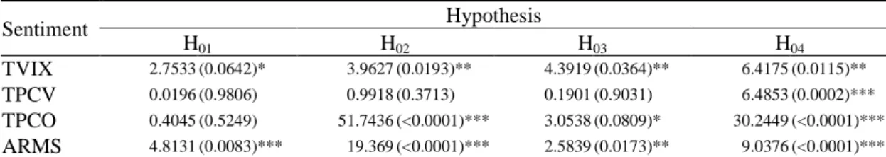
Table 5 Causality Tests between Returns and Sentiment – Sentiments Grouped at the Top, Median and Bottom Levels ... 23

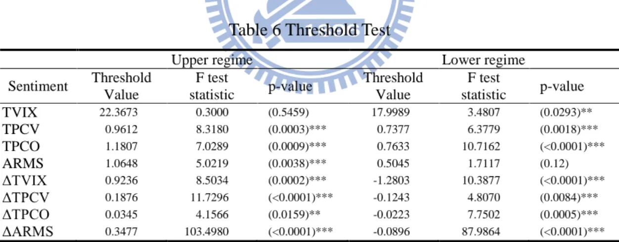
Table 6 Threshold Test ... 23

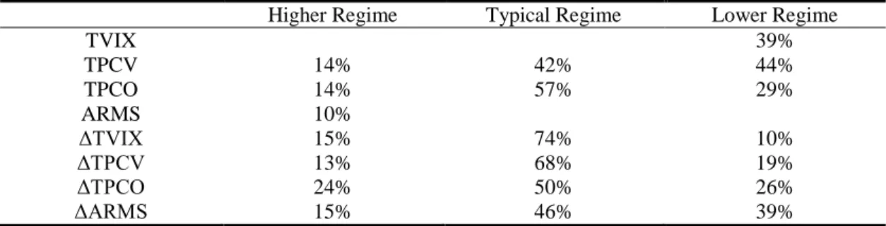
Table 7 Percentage of Each Regime Classified by Threshold Model ... 24

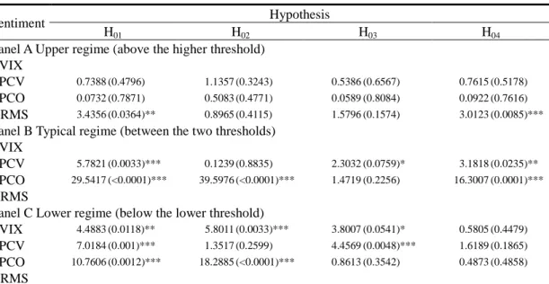
Table 8 Causality Tests between Returns and Sentiment - Application of the Multivariate Threshold Model ... 25

Table 9 Summary Statistics of the TAIEX, TVIIC, TVIIP and TVIIM ... 34

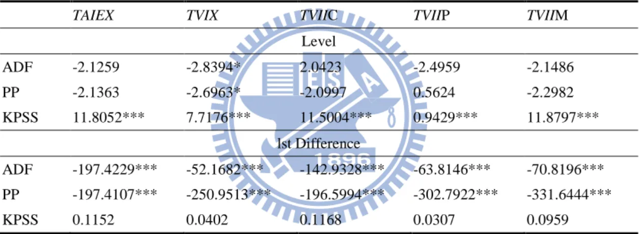
Table 10 Unit Root Tests ... 36

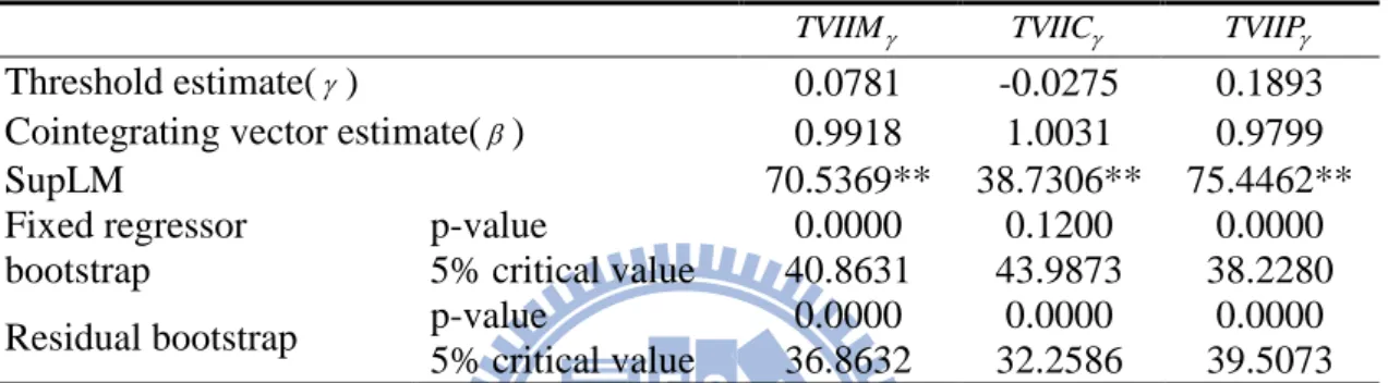
Table 11 Tests for the Threshold Effect ... 37

Table 12 Estimation of the Threshold VECM between TVIIM and TAIEX ... 38

Table 13 Estimation of the Threshold VECM between TVIIC and TAIEX ... 39

Table 14 Estimation of the Threshold VECM between TVIIP and TAIEX ... 40

Table 15 Correlation Coefficient and Causality Tests of the TVII and TAIEX in a Linear VECM ... 44

Table 16 Correlation Coefficient and Causality Tests of the TVII and TAIEX in a Threshold VECM ... 45

Table 17 Summary Statistics of Volatility and Investor Sentiment ... 51

Table 18 Correlation Coefficients of Volatility and Investor Sentiment ... 52

Table 19 Granger Causality Tests between Future Volatility and Sentiment ... 62

Table 20 Estimation Results of the Regression-Based Forecast Efficiency Test ... 64

Table 21 Forecast Evaluation of Volatility Models for h-day ahead Forecasts of Future Volatility Using MAPE ... 65

(11)

List of Figures

Figure 1 Daily Evolution of the TAIEX and TAIEX Returns ... 18

Figure 2 Daily Evolution of the Sentiment Indices ... 18

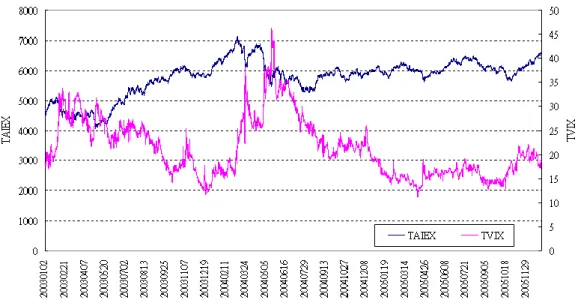
Figure 3 Fifteen-minute Evolution of the TAIEX and the Taiwan Volatility Index ... 34

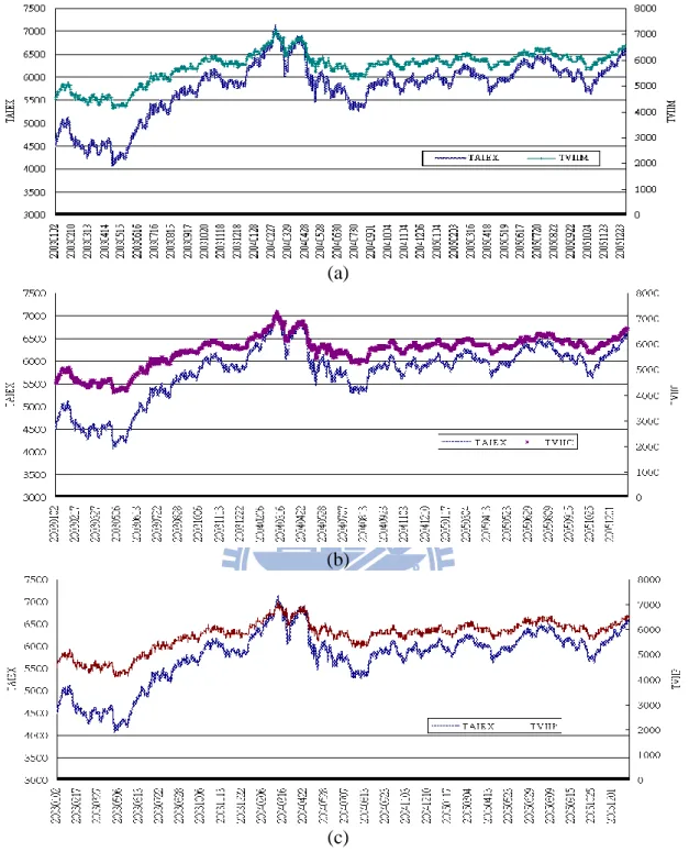
Figure 4 Fifteen-minute Evolution of the TAIEX and the Implied Index from the Taiwan Volatility Index... 35

Figure 5 Fifteen-minute Evolution of the Error Correction Term between the TVII and TAIEX ... 42

Figure 6 Daily Evolution of Future Volatility and Sentiment Indices ... 53

Figure 7 The Framework of Volatility Forecasting ... 57

(12)

Chapter 1. Introduction

The main purpose of this dissertation is to investigate the interaction among implied volatility, investor sentiment and market index from the behavioral finance point of view. An implied index from the options volatility is constructed under the Black-Scholes-Merton options pricing model which could serve as a proxy of the expected index level reflecting the investors‟ sentiment. The threshold model is applied to examine the extreme regimes of sentiment proxies and the causal relationship between investor sentiment and market index is examined under different market scenarios. Finally the forecasting model considering the information content of investor sentiment is performed and the options trading strategy is proposed. Based on the data of Taiwan stock market covering the period from 2003 to 2007, our results indicate that the information content of investor sentiment could be a leading indicator under overreaction and the strategy incorporating the sentiment proxies outperforms the other competitors.

Early papers (Friedman, 1953; Fama, 1965) argued that noise traders are unimportant in the financial price formation process because trades made by rational arbitrageurs drive prices close to their fundamental values. However, the market anomalies, for example, the under-reaction and overreaction of stock prices, challenge the efficient markets theory. De Long, Shleifer, Summers and Waldmann (DSSW (1990) hereafter) modeled the influence of noise trading on equilibrium prices and motivated empirical attempts to substantiate the proposition that „noise traders‟ risks influence price formation‟. Barberis, Shleifer and Vishny (1998) present a parsimonious model of investor sentiment. The model is based on psychological evidence and produces both underreaction and overreaction for a wide range of parameter values. If sentiment indicators are risk factors in the time series of returns, they will have the ability to predict the future returns on portfolios, even after appropriately adjusting for other risk factors. These findings support the need for research on the interaction between stock market returns, variation of price formation and indicators of investor sentiment.

Taiwan‟s equity market has long been an indispensable emerging market for international investors. Index options involving the Taiwan Stock Exchange Capitalization Weighted Stock Index (TAIEX index options, abbreviated as TXO)

(13)

were first traded on December 24, 2001. The TAIEX covers all of the listed stocks on the Taiwan Stock Exchange (TWSE) excluding preferred stocks, full-delivery stocks and newly-listed stocks, which are listed for less than one calendar month. The statistical data published in the 2007 annual report of the Futures Industry Association (FIA) show that the trading volume of Taiwan Stock Exchange Capitalization Weighted Stock Index options (TAIEX options) ranks twelfth in the world, which indicates its increasing importance for global asset management.1 The high trading percentage of individual traders in the Taiwan equity (about 70%) and derivatives (about 50%) markets might also imply that the noise trading or the investor sentiments might bethe cause of the price variations. This study therefore proceeds to examine the rapidly-developing Taiwan stock market.

There are three parts in this essay. They present three independent papers, respectively. In the first part of the dissertation, the causal relationships between sentiment and returns under different market scenarios are investigated. In contrast to previous studies that subjectively identify the bullish and bearish markets, we apply a threshold model to detect the extreme level of investors‟ sentiment econometrically. The empirical results show that most of the sentiment measures exhibit a feedback relationship with returns while ignoring different market states. However, sentiment could be a leading indicator if the higher or lower levels of sentiments were to be distinguished. Among them, the bullish/bearish indicator of ARMS, which is named after its creator, Richard Arms (1989), is a leading indicator if the market is more bearish (in the higher regime). Otherwise, the leading effect of the derivatives market sentiment indicators (the put-call trading volume and option volatility index) is discovered if the market is more bullish (in the lower regime). Our empirical findings further confirm the noise trader explanation that the causal direction would run from investors‟ sentiment to market behavior.

In the second part, the relationship between the information content implied by the options market-based volatility and the underlying stock index is analyzed through a threshold econometric model. A volatility index in line with the CBOE‟s new VIX is constructed by using intraday data for Taiwan‟s index options market as the research material. We then derive an implied equity index (TVII) from the Taiwan volatility

1

The FIA is the only association that is representative of all organizations having an interest in the futures market. The FIA has more than 180 corporate members, and reaches thousands of industry participants. Further information may be found on the website http://www.futuresindustry.org/.

(14)

index under the Black-Scholes-Merton options pricing scheme. We examine the co-movements and causalities between the TVII and the TAIEX (Taiwan stock exchange capitalization weighted stock index, TAIEX) through the vector error correction model (VECM) and threshold VECM (TVECM) in different market scenarios. The empirical results substantiate the claim that the nonlinear two-regime TVECM provides an appropriate fit for the dynamics between the TVII and the TAIEX. Investors participating in the Taiwan stock market could rebalance their equity portfolios while the implied index derived from the call options (TVIIC) takes precedence over the TAIEX.

In the last part, an algorithm for an effective option trading strategy based on superior volatility forecasts using actual option price data for the Taiwan stock market is proposed. The forecast evaluation supports the significant incremental explanatory power of investor sentiments in the fitting and forecasting of future volatility in relation to its adversarial multiple-factor model, especially the market turnover and volatility index which are referred to as the investors‟ mood gauge and proxy for overreaction. After taking into consideration the margin-based transaction cost, the simulated trading indicates that a long or short straddle 15 days before the options‟ final settlement day based on the 60-day in-sample-period volatility forecasting recruiting market turnover achieves the best average monthly return of 15.84%. This study bridges the gap between option trading, market volatility, and the signal of the investors‟ overreaction through the simulation of the option trading strategy. The trading algorithm based on the volatility forecasting recruiting investor sentiments could be further applied in electronic trading and other artificial intelligence decision support systems.

The remainder of this paper is organized as follows. Chapter 1 introduces the dissertation with the organization. Chapter 2 briefly discusses the relevant literature. Chapter 3 outlines the measurements of volatility and investor sentiment. Chapter 4 investigates the interaction between sentiment indicators and stock market returns under different market scenarios. Chapter 5 analyzes the interaction between the implied index from the options and the equity index in Taiwan. Chapter 6 proposes the options trading strategies based on volatility forecasting considering the investor sentiment. Finally, the conclusions drawn from this dissertation are presented in Chapter 7.

(15)

Chapter 2. Literature Review

2.1 Volatility Measures and Volatility Forecasting

Volatility is often defined as the (instantaneous) standard deviation (or „sigma‟) of the random Wiener-driven component in a continuous-time diffusion model. Volatility is a major parameter in risk management, derivatives pricing, options trading, hedging and asset allocation, and has also been one of the most active and successful areas of research in time series econometrics and economic forecasting in recent decades. Blair, Poon & Taylor (2001) and Poon & Granger (2003) have summarized that volatility forecasting models can be classified in the following four categories: the historical volatility models (HISVOL), the GARCH family, the options implied standard deviation (ISD) model, and the stochastic volatility model (SV).2

Over the past decade, several researchers have focused on the univariate analysis of volatility, such as the estimation and properties of volatility (e.g., Engle 1982, Taylor 1986, Bollerslev 1986, Andersen and Bollerslev 1998) and forecasts of volatility (e.g., Fleming et al. 1995, Koopman et al. 2005, Poon and Granger 2005). Other studies have focused on the multivariate analysis. Regardless of what categories of volatility are compared or composed, the main concerns of the forecasting model lie in investigating the possible indicators or properties which could improve the forecasting power and provide incremental information for application. The surveyed paper of Poon & Granger (2003, 2005) indicates that testing the effectiveness of a composite forecast is as important as testing the superiority of the individual models, but this has not been done more often or across different data sets. Multivariate forecasting models that consider the different categories of volatility models, such as the GARCH, historical volatility, stochastic volatility, and option implied volatility models, are constructed and compared hereafter (Engle & Gallo, 2006; Becker, Clements & White, 2007; Becker & Clements, 2008). In addition to the issue of the optimal combination of the multivariate volatility measures, there are other topics

2_{Historical volatility models (HISVOL) include those related to the random walk, historical averages}

of squared returns or absolute returns. Also included in this category are time series models which are based on historical volatility using moving averages, exponential weights, autoregressive models or fractionally integrated autoregressive absolute returns, etc. All models in the HISVOL group model volatility directly by omitting the goodness of fit of the returns distribution or any other variable such as the options price (Poon & Granger, 2003).

(16)

examining the possible indicators which could improve the predictive power of forecasting and its application.

2.2 Volatility and Market Index

Whaley (1993, 2000) and Fleming et al. (1995), for example, find a negative correlation between volatility and the market index. In addition, Copeland and Copeland (1999) show that volatility is a leading indicator of market returns.

Latané and Rendleman (1976), Chiras and Manaster (1978) and Beckers (1981) indicate that, when compared with the earliest methods, volatility which is derived from the options pricing model can be regarded as a good predictor of future volatility. There is also a growing volume of literature on the relationship between volatility and the market index. Wu (2001), Awartani and Corradi (2005) and Bollerslev et al. (2006) have recently claimed that causality between volatility and market index returns can be explained on the basis of the leverage effects (e.g., Black 1976) and volatility feedback (e.g., French et al. 1987).3 The nature of causality, which may be unidirectional or bi-directional, can be explained jointly by these two indistinguishable effects. Fleming et al. (1995) and Whaley (2000) point out that there is a highly negative correlation and asymmetric relationship between volatility and market index returns. In other words, losses lead to increases in volatility and gains result in decreases, but losses have a far greater impact on traded index volatility than gains. However, this is a direct violation of the predictions of classical finance theory.4 Montier (2002) claims that the asymmetric effect is just what the prospect theory, as proposed by Kahneman and Tversky (1979) in behavioral finance, would forecast.5

3_{The leverage effect indicates that a drop in the value of equity increases financial leverage, and this}

makes the equity riskier and thus increases its volatility. Volatility feedback means that if volatility is priced, an anticipated increase in volatility raises the required return on equity. Hence, the leverage effect prescribes a causal nexus from returns to conditional volatility, while volatility feedback prescribes one from conditional volatility to returns.

4_{Markowitz (1952) put forward the portfolio theory and assumed that risk was symmetric and could}

be expressed in terms of the standard deviation of asset returns.

5

The prospect theory, proposed by Kahneman and Tversky (1979) in behavioral finance, brings psychology into investors‟ decisions under uncertainty. It argues that investors have different risk tolerance in the face of gains and losses.

(17)

2.3 Investor Sentiment and Market Index

The causal relationships between sentiment indicators and stock market returns are mixed in previous studies. Clarke and Statman (1998) found that the sentiment of newsletter writers, whether bullish or bearish, does not forecast future returns, but that past returns and the volatility of those returns do affect sentiment. Causality would thus run from sentiment to market behavior if the noise trader explanation were to be accepted. However, Brown and Cliff (2004) and Solt and Statman (1988) documented that returns cause sentiment rather than the other way round. Brown and Cliff (2004) used a large number of sentiment indicators to investigate the relationship between sentiment and equity returns and found that returns cause sentiment rather than the opposite being the case. Brown (1999) supported the DSSW theory that irrational investors acting in concert and giving a noisy signal can influence asset prices and generate additional volatility. His tests used volatility instead of returns and his results indicated that deviations from the average level of sentiment are associated with increases in fund volatility only during trading hours. Lee, Jiang and Indro (2002) tested the impact of noise trader risk on the formation of conditional volatility and expected returns. Their empirical results show that sentiment is a systematic risk that is priced. Baker and Wurgler (2006) also indicated that investor sentiment affects the cross-section of stock returns. They found that when beginning-of-period proxies for sentiment are low, subsequent returns are relatively high for small stocks, young stocks, high volatility stocks, unprofitable stocks, non-dividend-paying stocks, extreme growth stocks and distressed stocks. Wang, Keswani and Taylor (2006) further tested the relationships between sentiment, returns and volatility. They also found strong and consistent evidence that sentiment measures, both in levels and first differences, are Granger-caused by returns. Banerjee, Doran and Peterson (2007) found that future returns are significantly related to both volatility index (VIX) levels and innovations for most portfolios, where the VIX is treated as a proxy variable for sentiment. While the causality test results presented above do not provide evidence of a consistent relationship between noise traders‟ sentiments and subsequent price movements, it might be possible that a relationship exists, but only in some special market scenarios.

The frame dependence theory, proposed by Shefrin (2000) in behavioral finance, argues that investors‟ decisions are sensitive to different market scenarios. This

(18)

motivates us to investigate whether there are dynamic causal relationships between sentiments and returns. Besides considering both positive and negative market scenarios, we infer that investors may exhibit dissimilar behaviors depending on the level of sentiment, and therefore different dynamic relationships may exist between stock market returns and sentiment indicators. Giot (2005) found that for very high (low) levels of the VIX, future returns are always positive (negative). His findings suggested that extremely high levels of the VIX might signal attractive buying opportunities. Banerjee et al. (2007) examined the relationship between returns and the VIX, the proxy variable for sentiment, for different levels of market performance and relatively high or low levels of volatility. Banerjee et al. (2007) defined those returns above and those below the sample median as constituting a „bull market‟ and a „bear market‟, respectively. Volatilities above the median level of the VIX are said to be in a „high volatility‟ period and those below the median in a „low volatility period‟. They provided two analyses, one of the „bull and bear market‟ and the other of „high and low volatility‟. Their findings suggested that the market states based on directional movements (positive and negative returns) or volatility levels (above or below the average) do not make a difference. On the contrary, we believe that the results will be misunderstood if the separation of the different market states is defined subjectively.

2.4 Volatility Forecasting and Investor Sentiment

From the behavioral finance point of view, the investors‟ behavior could be influenced by psychology or by bullish/bearish sentiment proxies (Montier, 2002; Shefrin, 2007). De Long, Shleifer, Summers, & Waldmann (DSSW (1990) hereafter) point out that investors are subject to sentiment and model the influence of noise trading on equilibrium prices. Their study motivates empirical attempts to substantiate the proposition that noise traders‟ risks indexed by sentiment influence either the mean or variance of asset returns. Sentiments are therefore proposed as one of the indicators which could enhance the incremental explanation of the future volatility.

A large body of literature focuses on the relationship and information content between returns and sentiment (Solt & Statman, 1988; DSSW, 1990; Clarke & Statman, 1998; Fisher & Statman, 2000; Wang, 2001; Simon & Wiggins, 2001; Brown & Cliff, 2004; Baker & Wurgler, 2006; Baker & Wurgler, 2007, Han, 2008).

(19)

While less attention is given to the impact of sentiments on the realized volatility or vice versa (Brown, 1999; Lee, Jiang & Indro, 2002; Low, 2004; Wang et al. 2006; Banerjee, Doran & Peterson, 2007; Verma & Verma, 2007), the exact role of sentiment in the price formation process is still a topic worth looking into.

To sum up, the information content of sentiment may be useful for volatility forecasting. However, the precise form in which sentiment will affect or predict volatility is not clear ex ante. For this reason, in our empirical analysis the possible sentiment indicators in the Taiwan stock market are constructed by referring to the previous literature, the predictive ability of sentiment to volatility is examined, the forecasting performance of the competitive models is compared, and finally effective option trading strategies are proposed based on the volatility forecasting.

2.5 Related Studies in Taiwan Stock Market

There are some related studies that focus on the Taiwan derivatives market. Lee, Lu and Chiang (2005) compare the characteristics and construction methodology of the volatility indexes across different countries. They find that the volatility index for the TAIEX (VXT) is a good estimator of future volatility. Besides, the VXT has negative and asymmetric relationship with the TAIEX and may be a contrarian trading signal when the market plunges. In contrast to Lee et al. (2005), the contribution of our study lies in the econometric analysis of the relationship between the information content of the volatility index and the TAIEX. Lee and Yuan (2005) investigate whether the traders‟ risk preference in the Taiwan stock market can be perceived by the volatility index. They find that investors in the Taiwan stock market tend to hedge the risk perception by put option contracts and the tendency is only remarkable in the bear market. Hsieh, Lee and Yuan (2006) separately construct the call and put implied volatility in the Taiwan Stock Market. Their empirical results show that put implied volatility is more closely linked to the spot index and is more sensitive to the change in the spot index than the call volatility. The strategy based on the information content of the put volatility index also outperforms the benchmark buy-and-hold strategy. In contrast to their study that the put volatility reveals more information content, our study indicates that the implied index derived from call options takes precedence over the underlying TAIEX.

(20)

Chapter 3. Volatility Measure and Investor sentiment

3.1 Volatility Measures

3.1.1 Future Volatility

In the framework of volatility forecasting, what exactly is forecasted is a key parameter. By referring to Corrado & Miller (2005), we employ the future realized volatility for the next h-days on day t, which is computed as the sample standard deviation of returns over the period from day t+1 through day t+h, and the future volatility is expressed in terms of the percentage annual term.6 The future realized return standard deviations are expressed as follows:

 

₂ 1/2 2 ; ; , 1 -1 S 252 ˆ ˆ FV R - R , R ln -1 S              _ _  _ _  



h t j t t T t T t j t t h t j j t j h   (3.1)

where Rt t h_, is the mean of the TAIEX return during days t+j to t+h, j=1,…h,

Rt+j represents the TAIEX market returns on day t+j, and St+j and St+j-1 are the daily

closing prices of the TAIEX on day t+j and t+j-1, respectively. The parameter h corresponds to the h-days-ahead volatility forecasting and it also equals h-days before the settlement day. Under this parameter, h is set as 5, 10, 15 and 20 days which exclude the weekends.

3.1.2 Historical Volatility Models

By referring to Engle & Gallo (2006), we jointly consider the three volatility measures, namely, absolute daily returns (|R|), daily high-low range (HL) and daily realized volatility (RV), as the benchmark forecasting model used in this study and it is simplified as MHV.7 Both the |R| and the HL are calculated using daily data,8 and

6_{By referring to John C. Hull (2006), this study assumes that there are 252 trading days in each year.} 7_{A multiple indicators volatility forecasting model jointly considers absolute daily returns (|R|), daily}

high-low range (HL) and daily realized volatility (RV) as proposed by Engle & Gallo (2006). The three variables have different features relative to one another, the main difference being that the daily return uses information regarding the closing price of the previous trading day, while the high-low spread and the realized volatility are measured on the basis of what is observed during the day. The former takes all trade information into account, and the latter is built on the basis of quotes sampled at discrete intervals.

8_{By taking the price limits in the Taiwan stock market into consideration}8_{, we transfer the high-low}

(21)

the RV is calculated by summing the corresponding five-minute interval squared returns9 (e.g., Andersen & Bollerslev, 1998; Barndorff-Nielsen & Shephard, 2002, among others), and the variable is expressed in terms of percentage annual terms. The calculations can be expressed as follows:



-1



R_t  ln S / S_t _t (3.2) 1 H L HL S_ 14%    t t t t (3.3) 2 0 -1 S RV ln 252 S       _ _   



n t i t i t i (3.4)

where |Rt| is absolute daily returns at time t, HLt is the daily high-low range

variation at time t, RVt is the daily realized volatility at time t, St is the closing price

on trading date t, St-1 is the closing price on the previous trading day, Ht is the highest

price on date t, Lt is the lowest price on date t, St+i is the intraday index level of the

i-th interval on trading day t, St+n represents the closing price on day t, i=0,…, n, and

n is the number of time intervals in each day.

3.1.3 Volatility Index

In 1993, the Chicago Board Options Exchange (CBOE) introduced the Volatility Index (VIX) based on the S&P 100 index options, which can be defined as the magnitude of price variations for the next 30 days. In 2003, the CBOE published the new VIX, which is based on the S&P 500 index options prices.10 The construction of the CBOE‟s new volatility index incorporates information from the skewness of volatility by using a wider range of strike prices including the out-of-the-money call and put option contracts rather than just the at-the-money series.11 The new VIX is

limits on day t in the Taiwan stock market are -7% and +7% of the previous day‟s closing price. Thus, the maximum price variation on day t would be 14% based on the previous day‟s closing price.

9_{The latest observations available before the five-minute marks from 09:00 until 13:30 are used to}

calculate the five-minute returns. We sum the 54 squared intra-day five-minute returns and the previous squared overnight returns to construct the daily realized volatility.

10

In March 2004, the CBOE futures exchange (CFE) introduced volatility futures, and volatility options were launched in February 2006. The underlying index is just the VIX published in 2003. The volatility index comprises tradable derivatives. The CBOE new VIX takes into account a wide range of strike prices for the same 30-day maturity, thus freeing its calculation from any specific option pricing model.

11_{For details of the index‟s construction, the interested reader may refer to the white book publish by}

(22)

not calculated from the Black-Scholes-Merton option pricing model which implies that the calculation is independent of any model. However, the fundamental features of the volatility index between the old and new versions remain the same. Since the new VIX is more precise and robust than the original version, we construct a volatility index for the Taiwan stock market based on the CBOE‟s last revision of the volatility index.

In the construction of the Taiwan stock market VIX, the interest rate has been adjusted accordingly. The risk-free rate is calculated from the monthly average one-year deposit rates at the Bank of Taiwan, Taiwan Cooperative Bank, First Bank, Hua Nan Bank and Chang Hwa Bank. The CBOE‟s volatility index (VIX) uses put and call options in the two nearest-term expiration months in order to bracket a 30-day calendar period. With 8 days left to expiration, CBOE‟s VIX „rolls‟ to the second and third contract months in order to minimize pricing anomalies that might occur close to expiration. However, the nearest-term expiration contract usually has high trading volume and the next nearest-term contract usually has low trading volume in the Taiwan options market even if the nearest-term contract is traded on the last trading day. In considering the market structure of liquidity and trading volume for the second and third contract months, we have revised the rollover rule from 8 days to 1 day prior to expiration in constructing the volatility index in Taiwan.

Options market-based implied volatility can reflect the expectations with respect to price changes in the future, and it can be treated as an indicator of sentiment. Olsen (1998) indicated that the volatility index has been viewed as a „sentiment indicator‟ in the recent behavioral finance literature and can be regarded as a market indicator of rises and falls in the underlying index. Whaley (2000) and research conducted by the Chicago Board Options Exchange (CBOE) have indicated that the greater the fear, the higher the VIX level is. Therefore, the volatility index is commonly referred to as the „investor fear gauge‟. Baker and Wurgler (2007) also treated option-implied volatility as one of the sentiment measures in investigating the investor sentiment approach. Therefore, the Taiwan stock market volatility index (TVIX) could be one of the volatility measures and one of the sentiment proxy variables in the Taiwan options market.

The hypothesis that volatility could reflect the expectations of future price changes and be treated as an indicator of sentiment is well documented (Whaley 2000, Baker and Wurgler 2006). Research by the Chicago Board of Options Exchange

(23)

(CBOE) indicates that, the greater the fear, the higher the Volatility Index (VIX) level is. The volatility index is therefore referred to as the “investor fear gauge”. Olsen (1998) indicates that the volatility index has been viewed as the “sentiment indicator” in the recent behavioral finance literature and can be a market indicator of rises and falls in index returns in the future.

3.2 The Construction of the Implied Index from the Options Volatility

Whaley (2000) indicates that the volatility index can be expressed as the „investors‟ fear gauge‟. The VIX is also treated as a proxy variable of investor sentiment in recent studies on behavioral finance (Baker and Wurgler, 2007; Banerjee, Doran and Peterson, 2007). Therefore the implied index derived from the TVIX can represent the investors‟ view of the underlying index under a certain level of the TVIX. The concept of the implied index proposed in this study from the TVIX is expressed below.

Implied volatility is volatility „implied‟ from an option price using the Black-Scholes-Merton options pricing model. It can be expressed as

( , , , , )

CBlsprice S K r T IV , where C is the call option price observed in the market. There are five parameters, S (underlying index), K (exercise price), r (risk-free rate), T (time to maturity) and IV (implied volatility). Here we substitute the volatility parameter as a Taiwan stock market volatility index (TVIX) and the implied index from the options volatility index can be derived from the call and put option prices as follows: ( , , , , ), ( , , , , ). i i i i K K i K K i

C Blsprice TVIIC K r T TVIX P Blsprice TVIIP K r T TVIX



 (3.5)

where K_i is the strike price, i1 X, X is the number of exercise contract traded on day t.

i K

TVIIC is the implied index derived from the call option at exercise

i K ,

i K

TVIIP is the implied index derived from the put option at exercise K_i, i K C is the midpoint of the bid-ask spread of the call option,

i K

P is the midpoint of the bid-ask spread of the put option, r is the risk-free rate and T is the time to maturity. Given TVIX, i K C ( i K

P ), K_i, r, T then the TVII= g-1(K_i,r, T, i K C ( i K P ), TVIX) is the information derived from the certain level of TVIX and we propose it as an implied

(24)

index from TVIX (TVII). TVII would not be equivalent to the underlying index, the

TAIEX, in the Taiwan stock market, since the TVIX is not derived from the

Black-Scholes option pricing model. To construct the TVIIC(TVIIP), we calculate the weighted average of

i K TVIIC (

i K

TVIIP ) based on the trading volume of each exercise. The construction is expressed as follows:

, , , , 1 1 , , , , 1 1 1 1 , / , , / , , / . N N C i Ki C i C i C i i i N N P i Ki P i P i P i i i M M i Ki i i i i i TVIIC w TVIIC w v v TVIIP w TVIIP w v v TVIIM w TVII w v v               



(3.6)

where N is the number of exercises, M is a 2× N vector which means that the

TVIIM contains information content regarding the contracts including the call and put

options, K_i is the exercise price,

i K

TVIIC is the implied index derived from the call option at exercise K_i,

i K

TVIIP is the implied index derived from the put option at

exercise K_i, vC i, is the trading volume of the call option at exercise Ki, vP i, is the

trading volume of the put option at exercise K_i, v_i is the trading volume of each contract including the call and put options at exercise K_i, w_{C i}_, is the weight of the call option at exercise K_i, wP i, is the weight of the put option at exercise Ki, wi

is the weight of each contract including the call and put options at exercise K_i, TVIIC represents the implied index which contains the information content of the call option, TVIIP is the implied index which contains the information content of the put option and TVIIM is the mean effect of TVIICand TVIIP.

3.3 Investor Sentiment

3.3.1 Put-Call Trading Volume and Open Interest Ratios

The put-call trading volume ratio equals the total trading volume of puts divided by the total trading volume of calls (TPCV). Like the TVIX, market participants view the TPCV as a fear indicator, with higher levels reflecting bearish sentiment. When market participants are bearish, they buy put options to hedge their equity positions or

(25)

to speculate bearishly. By contrast, a low level of TPCV is associated with a lower demand for puts, which reflects bullish sentiment.

The put-call open interest ratios can be calculated using the open interest of options instead of trading volume (TPCO). When the total option interest increases, most of it comes from higher investor demand for TXO puts. Thus the TPCO tends to be higher on days when the total open interest is high.

3.3.2 ARMS Index

The ARMS index is named after its creator, Richard Arms (1989), and is an indicator of bullish or bearish sentiment. The ARMS index on day t is equal to the number of advancing issues scaled by the trading volume (shares) of advancing issues divided by the number of declining issues scaled by the trading volume (shares) of declining issues. It is measured as:

t t t t

t

t t t t

#Adv /AdvVol DecVol /#Dec

ARMS = =

#Dec /DecVol AdvVol /#Adv (3.7)

where #Advt, #Dect, AdvVolt, and DecVolt, respectively, denote the number of advancing issues, the number of declining issues, the trading volume of advancing issues, and the trading volume of declining issues.

ARMS can be interpreted as the ratio of the number of advances to declines standardized by their respective volumes. If the index is greater than one, more trading is taking place in declining issues, while if it is less than one, the average volume of advancing stocks outpaces the average volume of declining stocks. Its creator, Richard Arms, argued that if the average volume of declining stocks far outweighs the average volume of rising stocks, then the market is oversold and this should be treated as a bullish sign. Likewise, he argued that if the average volume of rising stocks far outweighs the average volume of falling stocks, then the market is overbought and this should be treated as a bearish sign.

3.2.3 Market Turnover

Previous studies indicate that there is a relationship between trading volume (the turnover ratio) and stock market returns, and therefore it could be a trading signal (Campbell, Grossman & Wang, 1993; Cooper, 1999; and Gervais, Kaniel, &

(26)

Mingelgrin, 2001). On the other hand, trading volume, or more generally liquidity, can be viewed as an investor sentiment index (Scheinkman & Xiong, 2003; Baker & Stein, 2004; Baker & Wurgler, 2007). A high turnover ratio not only indicates that the market is dominated by irrational investors, but also implies that the market might be overreacting. Market turnover is calculated by the ratio of trading volume to the number of shares listed on the TWSE and is simplified as TO in this study. The data are fully quoted in the Taiwan Economic Journal (TEJ).

(27)

Chapter 4. Causalities between Sentiment Indicators and

Stock Market Returns under Different Market Scenarios

4.1 Introduction

The behavioral models of securities markets regard investors as being of two types: rational arbitrageurs who are sentiment-free and irrational traders who are prone to exogenous sentiment. In considering that investors may either overreact or under-react to extreme levels of sentiment indicators, we examine whether the sentiment indicators are classified according to multiple regimes by using the multivariate threshold model. Since previous studies have usually defined the extreme level subjectively, this paper analyzes the different states more objectively. The causality relationships between stock market returns and sentiment indicators are more significant when the different states are distinguished. The empirical results lead us to conclude that sentiment in both the stock and derivative markets gives rise to distinct lead-lag relationships with returns.

The analysis is conducted on a daily basis and the sentiment indicators used in this study include the TXO put-call trading volume ratio (TPCV), the TXO put-call open interest ratio (TPCO), the option market volatility index (TVIX) and the ARMS index. Our major focus of concern is on whether the causal relationship between sentiment and returns differs when investors‟ sentiment is at an extreme level identified optimistically by the threshold model. Our major findings suggest that there is nonlinearity in the sentiment indicators. The causality between sentiment and returns leads to different results when the sentiment index is at an extremely high or low level, or else reflects a typical regime. In the ordinary market scenario, there is low negative correlation as well as bi-directional causality. When the market overacts, the sentiment indicators Granger cause the returns. Among them, the ARMS index Granger causes the stock returns in the median and higher regimes, while the sentiment indicators in the derivatives market Granger cause the returns in the median and lower regimes. Our empirical findings further confirm the noise trader explanation that the causal direction runs from sentiment to market behavior.

To sum up, we apply the threshold model to examine the threshold effect of the sentiment indicators. Higher and lower regimes of sentiment indicators will be

(28)

detected objectively. Therefore, the causality relationship needs to be tested for different market scenarios.

4.2 Data

The daily sentiment indicators used consist of the TXO put-call trading volume ratio (TPCV), the TXO put-call open interest ratio (TPCO), the TXO volatility index (TVIX) and the TAIEX ARMS index. To do this, we use data that are fully quoted on the Taiwan Futures Exchange (TAIFEX) and the Taiwan Stock Exchange (TSE). The study period extends from 2003 to 2006, encompassing 993 trading days. Table 1 contains summary statistics of all the variables discussed in the study. The returns display excess kurtosis, negative skewness and almost no serial correlation. The contemporaneous relationships among many measures of investor sentiment and market returns depicted in Table 2 are shown to be strong. Figure 1 shows the daily evolution of the TAIEX and returns from 2003 to 2006. Figure 2 is the daily evolution of the sentiment indices from 2003 to 2006.

Table 1 Summary Statistics of Investor Sentiment and TAIEX Variable Mean Std. Dev. Skewness Kurtosis Autocorrelation

1  ₂ ₃ ₄ TAIEX 6,030.7580 732.2869 -0.4379 3.2624 0.9850 0.9700 0.9550 0.9410 R 0.0006 0.0120 -0.3855 6.3835 0.0390 -0.0110 0.0250 -0.0420 TVIX 20.7318 5.4899 0.9942 3.9072 0.9710 0.9530 0.9390 0.9230 TPCV 0.7835 0.1669 0.8043 4.3116 0.4640 0.3470 0.2820 0.2280 TPCO 0.9307 0.2597 1.1246 5.2412 0.9410 0.8720 0.8010 0.7370 ARMS 0.7168 0.3820 9.0595 175.3529 0.1190 0.0690 0.0010 -0.0120 ΔTVIX -0.0029 1.2995 1.2845 16.4393 -0.2030 -0.0490 0.0360 -0.0510 ΔTPCV 0.0004 0.1729 -0.0767 4.3869 -0.3920 -0.0550 -0.0050 -0.0220 ΔTPCO 0.0004 0.0885 -3.0162 35.3451 0.0870 0.0250 -0.0670 -0.0420 ΔARMS -0.0010 0.5087 -0.9781 91.5070 -0.4700 0.0110 -0.0320 0.0110

Notes: This table presents the summary statistics for the return on the Taiwan stock exchange capitalization weighted stock index (TAIEX) and various sentiment measures, namely, the Taiwan volatility index (TVIX), the put-call volume ratio (TPCV), the put-call open interest ratio (TPCO) and the ARMS ratio. The period covers 1/2/2003 to 12/29/2006.

Table 2 Contemporaneous Correlations of Investor Sentiment and TAIEX

R TVIX TPCV TPCO ARMS ΔTVIX ΔTPCV ΔTPCO ΔARMS

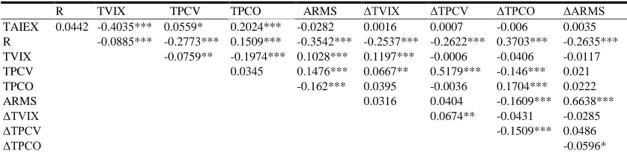
TAIEX 0.0442 -0.4035*** 0.0559* 0.2024*** -0.0282 0.0016 0.0007 -0.006 0.0035 R -0.0885*** -0.2773*** 0.1509*** -0.3542*** -0.2537*** -0.2622*** 0.3703*** -0.2635*** TVIX -0.0759** -0.1974*** 0.1028*** 0.1197*** -0.0006 -0.0406 -0.0117 TPCV 0.0345 0.1476*** 0.0667** 0.5179*** -0.146*** 0.021 TPCO -0.162*** 0.0395 -0.0036 0.1704*** 0.0222 ARMS 0.0316 0.0404 -0.1609*** 0.6638*** ΔTVIX 0.0674** -0.0431 -0.0285 ΔTPCV -0.1509*** 0.0486 ΔTPCO -0.0596*

Notes: The pairwise correlations are for selected variables used in the analysis. *, **, and *** indicate significance at the 10%, 5% and 1% levels, respectively.

(29)

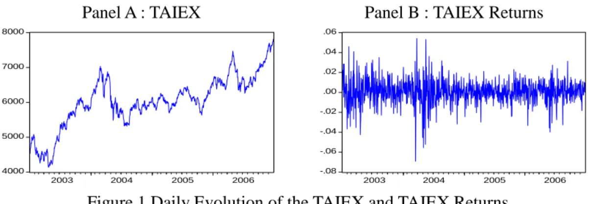
Panel A : TAIEX Panel B : TAIEX Returns

Figure 1 Daily Evolution of the TAIEX and TAIEX Returns

Notes: This figure shows the daily evolution of the TAIEX and TAIEX returns from 2003 to 2006. TAIEX represents the Taiwan stock exchange capitalization weighted stock index. TAIEX returns are calculated as the logarithmic difference in the daily TAIEX, i.e., Rt=lnSt-lnSt-1, where Rt represents the

TAIEX market returns on day t, and St and St-1 are the daily closing prices of the TAIEX on day t and

t-1, respectively.

Panel A : TVIX Panel B : TPCV

Panel C : TPCO Panel D : ARMS

Figure 2 Daily Evolution of the Sentiment Indices

Notes: This figure shows the daily investor sentiments during 2003 to 2006. The Taiwan volatility index (TVIX) is calculated using daily data quoted on the Taiwan Futures Exchange (TAIFEX) and the Taiwan Stock Exchange (TWSE). The method used to construct the TVIX refers to the essence of the last revision of the volatility index of the CBOE and the interest rate, and the rollover rule is revised accordingly. The ARMS, put-call trading volume ratio (TPCV) and put-call open interest ratio (TPCO) are calculated using daily data quoted on the TWSE and TAIFEX.

4.3 Research Design

4.3.1 Causality Tests

We test for Granger causality between sentiment and returns by estimating bivariate VAR models (Granger, 1969, 1988; Sims, 1972). The Granger causality tests

4000 5000 6000 7000 8000 2003 2004 2005 2006 -.08 -.06 -.04 -.02 .00 .02 .04 .06 2003 2004 2005 2006 10 15 20 25 30 35 40 45 50 2003 2004 2005 2006 0.4 0.6 0.8 1.0 1.2 1.4 1.6 1.8 2003 2004 2005 2006 0.4 0.8 1.2 1.6 2.0 2.4 2003 2004 2005 2006 0 1 2 3 4 5 6 7 8 9 2003 2004 2005 2006

(30)

examine whether the lags of one variable enter the equation to determine the dependent variables, assuming that the two series (sentiment index and stock market return) are covariance stationary and the error items are i.i.d. white noise errors.

We estimate the models using both levels and changes in sentiment measures since it is not easy to determine which specification should reveal the primary effects of sentiment. For example, suppose investor sentiment decreases from very bullish to bullish. One might anticipate a positive return due to the still bullish sentiment, but on the other hand, since sentiment has decreased, it is also possible for someone to expect a reduction in the return. The general model we use here can be expressed as follows: 1 1 1 1 1 1 2 2 2 2 1 1 , , L L t p t p p t p t p p L L t p t p p t p t p p R c a R b Senti Senti c a R b Senti                  



(4.1)

where Rt denotes the stock market returns and Sentit represents the sentiment

levels or the sentiment changes. The sentiment indices include TVIX, TPCV, TPCO and ARMS. In the bivariate Granger causality tests, the returns do not Granger cause the sentiment measures if the lagged values Rt-p do not enter the Sentit equation.

Similarly, the returns do not Granger cause the sentiment measures if all the a2p equal zero as a group based on a standard F-test. Meanwhile, the sentiment measures do not Granger cause the returns if all the b1p equal zero.

4.3.2 Causality Relationship under Different Market Scenarios

We examine the causality relationship under the positive and negative market return scenario. The model may alternatively be written as:

11 11 11 11 1 1 12 12 12 12 1 1 , if 0 L L t p t p p t p t p p t L L t p t p p t p t p p R c a R b Senti R Senti c a R b Senti            _ _ _ _   _   _ _ _ _ 



(4.2) 21 21 21 21 1 1 22 22 22 22 1 1 , if 0 L L t p t p p t p t p p t L L t p t p p t p t p p R c a R b Senti R Senti c a R b Senti            _ _ _ _   _   _ _ _ _ 



(4.3)

(31)

where Rt ≧0 represents the positive return scenario and Rt <0 is the negative

return scenario. The threshold variable of the return is also substituted as a sentiment variable. There are three scenarios examined in the following study, the extremely high sentiment (top 20%), the extremely low sentiment (bottom 20%) and the typical sentiment group (median 60%).

4.3.3 The Oversold and Overbought Scenarios Identified by the

Threshold Model

A two-regime version of the threshold autoregressive (TAR) model developed by Tong (1983) is expressed as follows:





-1 10 1 - 20 2 -1 1 -1 1, 1- , 0, p p t t t i t i t i t i i t i i t if y y I y I y I if y                 _  _ _  _ _{ }  



 



  (4.4)

where yt is the series of interest, θ 1i andθ 2iare the coefficients to be estimated,

i=1…p, p is the order of the TAR model, γ is the value of the threshold, and It is the

Heaviside indicator function. One problem with Tong (1983)‟s model is that the threshold may not be known. When γ is unknown, Chan (1993) shows how to obtain a super-consistent estimate of the threshold parameter. The general form of Chan‟s model can be described as:

10 11 -1 1 - 1 -20 21 -1 2 - 2 -, , t p t p t t d t t p t p t t d y y c e if y y y y c e if y                 _     (4.5)

For a TAR model, the procedure is to order the observations from the smallest to the largest such that y1 < y2 < y3 …< yT. For each value of yi, let γ=yi, and let the

Heaviside indicator be set according to this potential threshold in order to estimate a TAR model. The regression equation with the smallest residual sum of squares contains a consistent estimate of the threshold. Chan (1993) indicates that each data point within the band has the potential to be the threshold. However, it may be inefficient to examine the threshold effect of each value. Therefore, we adopt the grid search method whereby n sample points within the estimation period are selected to test the threshold effect and we set n equal to 100. In order to classify the oversold and overbought regimes, we apply the threshold test twice in the above and below average levels of each sentiment indicator. The highest and lowest 10 percent of the

隱含波動度, 投資人情緒與市場指數之互動關係與策略應用

國立交通大學

管理科學系

博 士 論 文

No. 054

隱含波動度, 投資人情緒與市場指數之

互動關係與策略應用

The Interaction and Strategy Application between

Implied Volatility, Investor Sentiment and Market Index

研 究 生：魏裕珍

指導教授：許和鈞 教授

國立交通大學

管理科學系

博 士 論 文

No. 054

隱含波動度, 投資人情緒與市場指數之

互動關係與策略應用

The Interaction and Strategy Application between

Implied Volatility, Investor Sentiment and Market Index

研 究 生：魏裕珍

研究指導委員會：謝國文 教授

研究指導委員會：

鍾惠民 教授

指導教授：許和鈞 教授

隱含波動度, 投資人情緒與市場指數之

互動關係與策略應用

The Interaction and Strategy Application between

Implied Volatility, Investor Sentiment and Market Index

研 究 生：魏裕珍

Student：Yu-Chen Wei

指導教授：許和鈞

Advisor：Her-Jiun Sheu

國 立 交 通 大 學

管 理 科 學 系

博 士 論 文

A Dissertation

Submitted to Department of Management Science

College of Management

National Chiao Tung University

in Partial Fulfillment of the Requirements

for the Degree of

Doctor of Philosophy

in

Management

July 2010

Hsin-Chu, Taiwan, Republic of China

隱含波動度, 投資人情緒與市場指數之

互動關係與策略應用

研究生：魏裕珍

指導教授：許和鈞

國立交通大學管理科學系博士班

中文摘要

The Interaction and Strategy Application between

Implied Volatility, Investor Sentiment and Market Index

Student：Yu-Chen Wei

Advisor：Her-Jiun Sheu

Department of Management Science

National Chiao Tung University

Abstract

致謝辭

Table of Contents

List of Tables

List of Figures

Chapter 1. Introduction

Chapter 2. Literature Review

2.1 Volatility Measures and Volatility Forecasting

2.2 Volatility and Market Index

2.3 Investor Sentiment and Market Index

2.4 Volatility Forecasting and Investor Sentiment

2.5 Related Studies in Taiwan Stock Market

Chapter 3. Volatility Measure and Investor sentiment

3.1 Volatility Measures

3.1.1 Future Volatility

 



3.1.2 Historical Volatility Models







3.1.3 Volatility Index

博士論文

研究生：魏裕珍

指導教授：許和鈞教授

博士論文

研究生：魏裕珍

研究指導委員會：謝國文教授

鍾惠民教授

指導教授：許和鈞教授

研究生：魏裕珍

國立交通大學

管理科學系

博士論文