針對建構有限長度之PEG 類型演算法效能改善之研究

國

立

交

通

大

學

電信工程研究所

碩

士

論

文

針對建構有限長度之 PEG 類型演算法效能改善之研究

Performance Improvement of PEG-based Construction for Finite-Length

LDPC Codes

研 究 生：杜建東

指導教授：王忠炫 教授

針對建構有限長度之 PEG 類型演算法效能改善之研究

Performance Improvement of PEG-based Construction for Finite-Length

LDPC Codes

研 究 生：杜建東 Student：Jian-Dong Du

指導教授：王忠炫 Advisor：Chung-Hsuan Wang

國 立 交 通 大 學

電信工程研究所

碩 士 論 文

Submitted to Institute of Communication Engineering College of Electrical and Computer Engineering

National Chiao Tung University in partial Fulfillment of the Requirements

for the Degree of Master

in

Communication Engineering

July 2012

tt

針

針

針

_對

_對

_對建

建

建構

構

構有

有

有限

限

限長

長

長度

度

度之

之

之PEG類

類

類型

型

型演

演

演

算

算

_算法

_法

_法效

效

效能

能

能改

改

改善

善

善之

之

之研

研

研究

究

究

PEG演算_{法是一種常見而且簡單被用來建構large girth之有限長度的低密度奇偶檢查碼}

的方法。然而，我們發現PEG演算法在架構上有不足的地方，導致每次在Tanner graph上 生長edge時無法把產生的cycle長度拉得更大，因此傷害了解碼效能。為了克服這樣不足 的地方，這這篇論文中介紹了兩個方法。我們以前人的演算法為基礎，並運用這兩個方 法，提出了兩個修改後的新演算法。此外，我們介紹了一個序列，這個序列透露了某 些degree的variable node之間存在的cycle長度。從數據的結果顯示，我們的方法可以有效 的拉大這個序列中的數值。而且這個數列不但可以簡單的區別Tanner graph的好壞，也可 以提供給我們造碼的方向。從結果顯示，我們提出的演算法可以有效的改善cycle的連結 性，因此效能能夠有一定程度的改善。

Performance Improvement of PEG-based Construction

for Finite-Length LDPC Codes

Student: Jian-Dong Du kkkAdvisor: Chung-Hsuan Wang

Institute of Communications Engineering National Chiao Tung University

Abstract

The progressive-edge-growth (PEG) algorithm is a well-known simple approach to con-struct finite length LDPC codes with large girth. However, we find that the PEG algorithm has some fundamental weaknesses, which limit the maximum achievable cycle length of each edge grows in Tanner graph and hence hurt the decoding performance. To overcome the weaknesses, two strategies for the PEG algorithm are proposed in this thesis. With these strategies, we proposed two algorithms modified from the PEG algorithm and the improved PEG algorithm respectively. In addition, we introduce a cycle length sequence which coveys the cycle length information between variable nodes with different degree. The obtained results confirm that our strategies can effectively increase the cycle length sequence. This sequence is not only useful for discriminating a Tanner graph, but also valuable to provide new insights for code construction. Our results also show that the proposed algorithms can considerably improve the connectivity of cycles, and thus the performance is improved to some extent.

Acknowledgements

Contents

2 Background of PEG-based Algorithms 5

2.1 LDPC Codes and The Tanner Graph . . . 5

2.2 The PEG Algorithm [6] . . . 7

2.3 The Improved PEG Algorithm [14] . . . 8

2.4 The Variable Node ACE Spectrum . . . 10

2.5 The Other Factor That Influence on The BER Performance . . . 11

Strate-gies 13

3.1 The Cycle Length-on-Edge Sequence (CLoES) . . . 14

3.2 The First Strategy for Cycle Length-Boosting: First Edge Selection Refine-ment . . . 16

3.3 The Second Strategy for Cycle Length-Boosting: Node-grouping for Selection of The Other Edges . . . 17

3.4 The Modified PEG Algorithm . . . 19

3.5 The Modified Improved PEG Algorithm . . . 21

3.6 The Other Topics . . . 23

3.6.1 The First Topic . . . 23

3.6.2 The Second Topic . . . 24

4 Numerical Results and Discussions 26 4.1 Discussions for The Two Strategies . . . 26

4.2 Discussions for The Proposed Algorithms . . . 29

5 Conclusion Remarks and Future Work 40

List of Figures

2.1 Parity check matrix H and the Tanner graph are equivalent. . . . 6

2.2 A cycle with length six is indicated here. . . 7

2.3 The procedure of the PEG algorithm (S5 grows its second edge). . . 9

2.4 The performances are sensitive to the connecting of low-degree variable nodes.

FERs over the AWGN channel, (n=1008 and rate=1/2) . . . 12

3.1 What is the best way to connect edge between variable node and check node? Is it really a good way for PEG to achieve that? . . . 14 3.2 Original PEG (S3 choose the first edge): Direct select minimum degree

sur-vivor. For this case, C0 and C2 are candidates. . . 16 3.3 The procedure of the second strategy for a group (t = 3 in this case). . . . . 19

4.1 BERs for the PEG algorithm modified by the first strategy (n=1008 and

rate=1/2) . . . 27

4.2 BERs for the Improved PEG algorithm modified by the first strategy (n=1008

and rate=1/2) . . . 28 4.3 BERs for the PEG algorithm modified by the second strategy with group sizes

4.4 Decay on the CLoESs of the original PEG algorithm and the PEG algorithm modified by the second strategy . . . 31

4.5 Decay on the E(3) _{of the original PEG algorithm and the PEG algorithm}

modified by the second strategy . . . 32

4.6 BERs for the modified PEG algorithm (n=2016 and 1008, rate=1/2) . . . . 34

4.7 Decay on the CLoESs of the improved PEG algorithm and the modified

im-proved PEG algorithm . . . 35

4.8 Decay on the E(3)_{of the improved PEG algorithm and the modified improved}

PEG algorithm . . . 36

4.9 BERs for the modified improved PEG algorithm (n=1008 and rate=1/2) . . 37

4.10 BERs for the modified improved PEG algorithm (n=2016 and rate=1/2) . . 38

Chapter 1

Introduction

Low-density parity-check (LDPC) code is an attractive error correction code [1]. Its bit-error-rate (BER) performance has been shown to achieve Shannon limit with an infinite codeword length and an iterative decoding algorithm based on belief propagation, e.g., the sum-product algorithm (SPA) [1]. However, in practical consideration, the codeword length is finite and usually ranges between several hundreds and several thousands. In this range, a randomly generated parity-check matrix which satisfies the capacity-approaching degree distribution will easily comprise some unfavorable structures, such as the stopping sets [2] trapping sets [3], and absorbing sets [4], etc. Moreover, due to the existence of those structures, the decoding based on the Tanner graph corresponding to that parity-check matrix and the SPA is frequently observed to have an unacceptable BER performance, especially at the high signal-to-noise ratio (SNR) region. Therefore, to make LDPC codes suitable for realistic requirements, the finite length construction of a parity-check matrix is undoubtedly an important issue.

After years of effort, several guidelines were successively proposed to construct finite length LDPC codes [5]- [7]. From the Tanner graph perspective, those guidelines suggest: (1)enlarging the girth; (2)maximizing the length of cycles between low degree variable nodes; (3)increasing the extrinsic messages degree (EMD) or the approximated cycle EMD (ACE)

for short cycles; (4)avoiding generating small stopping sets or the elementary trapping sets. To adopt the above suggestions, an intelligent framework provided by the progressive-edge-growth (PEG) algorithm [6] is shown to be extremely effective. On the other hand, the algebraic constructions of parity-check matrix are attractive. This class of LDPC codes often has quasi-cyclic property that is favorable for hardware implementations.

In short, the main idea of the PEG framework is to construct a Tanner graph progres-sively, one edge at a time, one node after another. By this, in the PEG algorithm, the first edge of each variable node is proposed to connect with a check node which has the smallest degree under the current graph setting; for other edges, each edge is grown to maximize the girth. Consequently, a graph with large girth can be obtained.

Like other various construction methods, the PEG algorithm still suffer from the exis-tence of error floor [3]. Owing to the nice girth property on the resulting graph, the PEG algorithm is also employed as a base and combined with different strategies to achieve bet-ter performance or other purposes [7]- [14]. In [7], [8], methods for constructing irregular LDPC codes without small stopping sets were presented. To construct completely regular codes without lowering the girth, an algorithm was proposed in [9]. In [10], an independent tree-based method for lower bounding the minimum distance of low-density parity-check codes is presented. A modified PEG algorithm for construction of LDPC codes with strictly concentrated check node degrees is proposed in [11]. A modification of the PEG algorithm that improves the performance in the waterfall region is described in [12]. A modified PEG algorithm with polynomial of cycle, which achieves not only large girth, but also minimizes the number of the shortest cycles significantly is proposed in [13]. In [5], it is shown that the connectivity of the cycles also plays an important role on the BER performance in the error floor region. To distinguish the connectivity of the cycles, the approximated cycle extrinsic message degree (ACE) metric was introduced. The authors in [14] proposed the improved

PEG algorithm which maximizing the girth and improving the ACE metric of the cycles. The improved PEG algorithm is paid much attentions owing to its simplicity and effective-ness. In their modified algorithm, it often happens that one has a few candidate check nodes to connect to a given variable node (all such candidates result in the same local girth under the current graph). Among the candidate check nodes, a check node which has the largest minimum path ACE metric is chosen.

Even though the improved PEG algorithm gains some improvements at error floor region, we find that the improved PEG algorithm itself leaves some room to improve. Several con-tributions are hence made in this thesis. First of all, to make the cycle length be maximized at each growth step, we propose that the first edge selection of each variable node should be jointly optimized with the second edge selection, instead of randomly connecting with a check node that has the lowest degree. Second, we suggest to relax the node-by-node growth in the PEG algorithm with a nodes-by-nodes approach during construction, i.e., an edge is selected to grow among a group of variable nodes rather than only one node. It is then possible to further increase the cycle length when cycles are formed. Based on the above two strategies, it is straightforward to refine the PEG algorithm accordingly. To further improve the performance of the improved PEG algorithm, we also propose an algorithm which can further enlarge the cycle length and ACE simultaneously when cycles are formed. On the other hand, we introduce a sequence so-called cycle length-on-edge sequence (CLoES). This sequence is useful to understand the length of cycles between variable nodes with certain degrees. As a result, this sequence can be somehow as a measurement for discriminating a Tanner graph and may provide a new viewpoint for constructing LDPC codes.

The rest of this thesis is organized as follows. In following chapter, we introduce the background of the PEG-based algorithms. The CLoES and our modifications to the PEG algorithm and the improved PEG algorithm are presented in Chapter 3. In Chapter 4, some

simulation results are provided for verification. Finally, a summary is drawn in Chapter 5 to conclude this work.

Chapter 2

Background of PEG-based Algorithms

In this thesis, besides the original PEG algorithm, we name any algorithm modified based on the original PEG algorithm as the PEG-based algorithm. This chapter gives a brief overview of the notations and definitions related to the PEG-based algorithm. Specifically, Section 2.1 introduces some definitions related to the Tanner graph. The original PEG algorithm and the improved PEG algorithm are introduced in Section 2.2 and Section 2.3 respectively. In Section 2.4, the variable node ACE spectrum is introduced. Moreover, by giving an example, beside the girth histogram and the variable node ACE spectrum, the other factor that may influence on the BER performance is introduced in Section 2.5.

2.1

LDPC Codes and The Tanner Graph

An LDPC block code is defined as the null space of an m-by-n sparse parity-check matrix

H. The Tanner graph G(H) associated with H is a bipartite graph. In G(H), there

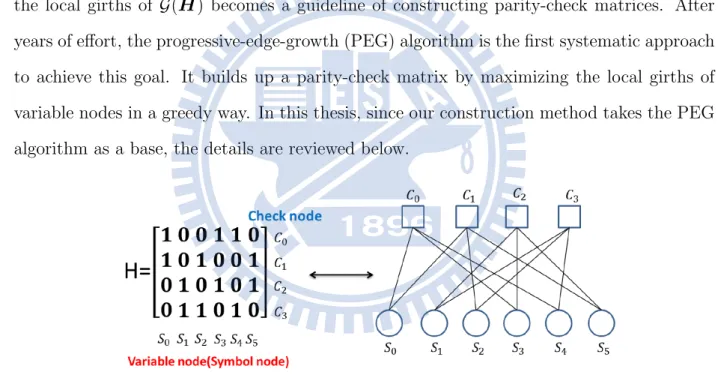
are n variable nodes and m check nodes, which are corresponding to the columns and the rows of H, respectively. The connections between the variable nodes and the check nodes are specified by the nonzero entries in H. The equivalent of H and the Tanner graph is depicted in Fig. 2.1. Moreover, a cycle in G(H) is defined as a path that starts and ends at

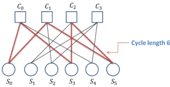
the same node, and any edge in between appears only once. The cycle length is the number of edges that are contained in a cycle. The girth is the shortest cycle length in G(H); the

local girth of a variable node is the shortest cycle length which involves that node. Fig. 2.2

indicates a cycle with length six in a Tanner graph.

Decoding of LDPC code based on G(H) and the SPA, the girth was firstly observed to

be an important factor that affects the decoding performance [1]. Furthermore, the girth histogram, which conveys the information of all local girths of variable nodes, was later found of greater influence on the BER performance than the girth [15]. Short cycle in the Tanner graph will easily degrade the performance of LDPC codes. Due to this discovery, enlarging the local girths of G(H) becomes a guideline of constructing parity-check matrices. After years of effort, the progressive-edge-growth (PEG) algorithm is the first systematic approach to achieve this goal. It builds up a parity-check matrix by maximizing the local girths of variable nodes in a greedy way. In this thesis, since our construction method takes the PEG algorithm as a base, the details are reviewed below.

Figure 2.2: A cycle with length six is indicated here.

2.2

The PEG Algorithm [6]

To construct a parity-check matrix H, the codeword length n and the code rate R are given at first. For this code rate, a technique so-called density evolution is then used to optimize the variable node degree distribution [16], in which the degree of a node is defined as the number of edges incident to that node. Let λi be the fraction of variable nodes of

degree-i. Denoted by dmaxand dmin the maximum and the minimum degree of variable node, respectively. The variable node degree distribution is of the following form:

λ(X) =

d∑max

i=dmin

λiXi.

From λ(X), it can be seen that there are totally n· λi variable nodes of degree-i in G(H).

Note that n· λi is always a fraction. Without loss generality, we round up the fraction into

an integer.

Letting variable nodes in G(H) be labelled and ordered according to their degree in a non-decreasing order, we define the variable node degree sequence DS , {ds1, ds2,· · · , dsn |

ds1 ≤ ds2 ≤ · · · ≤ dsn}, where the subscript sj denotes the label of the jth variable node and

dsj is the degree of sj. On the other hand, there are m = n· (1 − R) check nodes in G(H).

Let Nl

sj represent the set of check nodes which can be reached by expanding a tree from sj

within depth l, and let Nl_s

j be the complement set of N

l

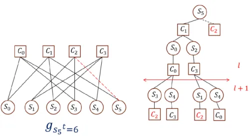
illustrates the behaviour of expanding a tree from S5 within depth l and the procedure of growing an edge. With DS, the PEG algorithm executes the following procedure to generate

H.

The PEG Algorithm:

• for j = 1 → n

– for k = 1→ dsj

∗ if k = 1

· Connect the first edge of sj with a check node, which has the lowest check

node degree under the current graph setting.

∗ else

· Expand a tree from sj up to depth l under the current graph setting such

that Nl_sj ̸= ∅ but Nl+1_sj =∅, or the cardinality of N_sl_j stops increasing but is less than m. Connect the k-th edge of sj with a check node from N

l sj

that has the lowest degree.

∗ end if

– end for

• end for

2.3

The Improved PEG Algorithm [14]

With the great success of the PEG algorithm, many girth-conditioning constructions were successively presented to further avoid producing some structures, such as the stopping sets or the trapping sets, in a parity-check matrix [2], [3]. Among those rich studies, a novel

Figure 2.3: The procedure of the PEG algorithm (S5 grows its second edge).

perspective emphasizes that not only the cycle length, but also the connectivity of cycles plays an important role on the BER performance in the error floor region. It is also pointed out that not all short cycles of the same length are equally harmful for decoding. Hence, the authors in [5] introduced a metric, called approximated cycle extrinsic message degree (ACE), to measure the connectivity and the harmfulness of a cycle.

By definition, the ACE of a cycle is∑_j(dsj− 2), in which the sj’s are the variable nodes

contained in that cycle [5]. A cycle with the larger ACE implies that it has more connections with the rest of Tanner graph. The variable nodes in that cycle can obtain much extrinsic information outside the cycle and might pass more reliable messages along the cycle. Thus, this cycle is less harmful for decoding in general. Based on this, the edge connection except for the first edge in the PEG algorithm is modified to choose the check node that can create both the largest local girth and the ACE. This modification is well-known as the improved

2.4

The Variable Node ACE Spectrum

In order to distinguish the ACE property of LDPC codes, in [17], given a variable node sj,

G(H) and L , a variable node ACE spectrum associated with the variable node sj in the

Tanner graph G(H) is a L-tuple vector: ηsj(G(H)) = (η

sj 2 , η sj 4 ,· · · , η sj 2L), where η sj 2i denotes the minimum ACE metric over the set of cycles which length are 2i and pass through variable node sj.

Since the shortest cycles with small ACE metric are of greater harmful than those longer cycles for the performance of iterative decoding, in this thesis, we simplify a variable node

ACE spectrum. For a variable node sj, we only consider the minimum ACE metric of the

shortest cycles. i.e.,

¯

ηsj(G(H)) = η

sj

g_sj

, where gsj denotes the local girth of variable node sj.

We then modify the variable node ACE spectrum (VN-ACES) by ¯

η(G(H)) = (ηs1

g_s1, ηgs2_s2,· · · , ηgssnn ) for a careful inspection, where η

sj

g_sj is the minimum ACE

over the set of the shortest cycles pass through sj.

Also, we define ¯ηi ¯ ηi = 1 nλi ∑ j:d_sj=i ηsj lmin

as the average ACE of degree-i variable nodes. With this measurement, we can generally evaluate the good or bad in connectivity for certain degree variable nodes. With the girth histogram, the modified VN-ACES and ηi’s can be useful to evaluate the goodness of a code.

The larger values in the modified VN-ACES, the cycles generally have better connectivity in the Tanner graph, and the performance of the code more likely is better. In Chapter 4, we will make use of it to compare the ACE property of LDPC codes.

2.5

The Other Factor That Influence on The BER

Per-formance

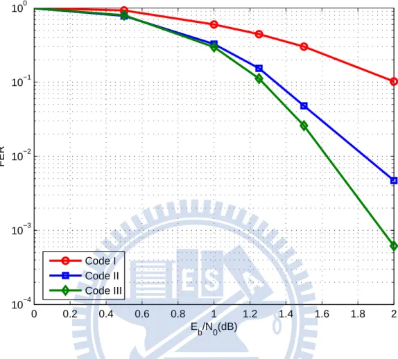
Here, we give an example to explain that girth histograms are not enough to compare the performance of LDPC codes. In Fig. 2.4, there are three different LDPC codes of length n=1008, Rate=1/2, and all with the same variable node degree distribution which is given by λ(x) = 0.47532x2 + 0.279537x3 + 0.0348672x4 + 0.108891x5 + 0.101385x15. Code I is constructed by randomly establishing edges and avoiding cycles of length four. Code II is constructed by connecting all degree-2 variable nodes in a zigzag manner to avoid cycles between degree-2 variable nodes. The other edges are selected randomly by avoiding cycles of length four. Code III is constructed with the original PEG algorithm.

These three codes have the same girth histogram, i.e, the local girth for all variable nodes are 6 in these three codes. However, the difference in the code construction procedure lead to the large gap in the performances of these three codes. It can be seen that the performance of the second code is better than that of the first code, because the first code exists short cycles between degree-2 variable nodes, but the second code has no cycle between degree-2 variable nodes. The performance of the third code is even better than that of the second code, since the third code has mostly longer cycles between low-degree variable nodes compare to the second code.

From the ACE perspective, while short cycles are formed between low-degree variable nodes, these short cycles will have small ACE metric. Therefore, the performance of LDPC codes will degrade seriously. Based on this observation, we can find that it is important to avoid short cycles being formed between low-degree variable nodes. Even through the girth histogram is important for the performance of the LDPC codes in most case, but it is not absolute. Except for the girth histogram, we should also pay attention to those low-degree variable nodes; such like find out how short are the cycle lengths exist between

0 0.2 0.4 0.6 0.8 1 1.2 1.4 1.6 1.8 2 10−4 10−3 10−2 10−1 100 E_b/N₀(dB) FER Code I Code II Code III

Figure 2.4: The performances are sensitive to the connecting of low-degree variable nodes. FERs over the AWGN channel, (n=1008 and rate=1/2)

low-degree variable nodes. In the beginning of the next chapter, a method for gathering such information will be presented. Later, we will also propose algorithms which can increase the cycle lengths exist between low-degree variable nodes.

Chapter 3

The Cycle Length-on-Edge Sequence

and The Cycle Length-Boosting

Strategies

From Fig. 3.1, we can image that here having a space, and in which are variable nodes and check nodes. Now giving us the number of edges, how should we put this edges between variable nodes and check nodes for obtaining the largest girth and the best connectivity simultaneously in this graph? Is PEG really a good way for achieving such a purpose? Or how to do? Thus, we proposed several algorithms for solving such a problem in this chapter. In literature, the girth histogram and the VN-ACES are two primary measurements for a Tanner graph. Except for their formal definitions, they also offer some additional information to the decoding by the SPA. For example, the girth histogram can indicate how many iterations a variable node will receive dependent messages, and the VN-ACES can reflect how many opportunities the messages passed in a cycle can be improved with the extrinsic information from the check nodes outside the cycle. However, if we are asked how are the connections between the variable nodes with different degree in a Tanner graph, there will be no answer to this important question based on the above two measurements. Hence, in Section 3.1, we introduce a sequence to provide such knowledge for PEG-based

Figure 3.1: What is the best way to connect edge between variable node and check node? Is it really a good way for PEG to achieve that?

algorithms.

In addition, we present two strategies to enlarge cycle lengths from the new knowledge perspective in the Section 3.2 and Section 3.3 respectively. In Section 3.4, we modify the original PEG algorithm by using our two strategies. An algorithm modified from the im-proved PEG algorithm is proposed in Section 3.5. Furthermore, the other research contents will be mentioned in Section 3.6.

3.1

The Cycle Length-on-Edge Sequence (CLoES)

Owing to the progressive-edge-growth nature of PEG-based algorithms, the length of the shortest cycle that passes through a newly grown edge under the current Tanner graph is known. This length is of great interest because it shows the shortest cycle length between the current growing variable node and the other nodes that have grown edges. If no cycle is formed, the shortest cycle length associated with the newly grown edge is defined as infinity. By this definition, the first edge of each variable node has an infinite cycle length. Therefore,

only the shortest cycle lengths on all edges other than the first edge of a node are informative. During the process of growing the edges of all degree-d variable nodes, except for the first edge of each node, we let E(d) , [E(d)

1 , E (d) 2 ,· · · , E (d) i ,· · · , E (d) zd ], where E (d) i denotes the

shortest cycle length corresponding to the ith edge growth, and zd stands for the step index

of the last edge growth of the degree-d variable nodes. The cycle length-on-edge sequence (CLoES) is then defined as E = [E(dmin)_{, E}(dmin+1)_,· · · , E(dmax)_{]. The values of E can be}

obtained during the construction.

For the CLoES, the most significant feature is that it can be used to inspect the con-nections between some variable nodes. For example, the values in E(d) shows that how an edge of a degree-d variable node constitutes a cycle with the other nodes that have smaller or the same degree. Since the cycle length between variable nodes is critical to the BER performance, it is thus desired to enlarge the values in E, especially the values in E(d)_{’s with} small d’s due to the fatal defects of the cycles that comprises only low-degree variable nodes.

For convenient comparison between different E, we also define Ωd, {i : E

(d) i ̸= ∞, ∀ 1 ≤ i ≤ zd} and let ¯E(d) = ∑ i∈ΩdE (d)

i /|Ωd|, in which |Ωd| is the cardinalities of set Ωd. ¯E(d) is

the average cycle length of E(d) _{and ¯E is the average of ¯E}(d)_{’s. ¯E}(d) _{can generally reflect the} connection between the variable node with degree no more than d. In addition, the larger the ¯E is, the average cycle length is relatively longer in graph. Thus, we prefer to construct a

graph with larger ¯E(d) and ¯E. After we modify an algorithm, we expect that the most values

in E may increase respect to the original version algorithm. To confirm such expectation, we calculate the amount of the increased values and the decreased values in E, then the

ratio is defined as the first amount to the second amount. The larger the ratio is, the larger

probability the modified algorithm works well. To increase the cycle length between variable nodes, or equivalently to enlarge the values in E, in the following section, we propose two novel strategies for PEG-based algorithms. One strategy is to refine the first edge connection

of a variable node, while the other one is to grow edges with respect to a group of nodes.

3.2

The First Strategy for Cycle Length-Boosting: First

Edge Selection Refinement

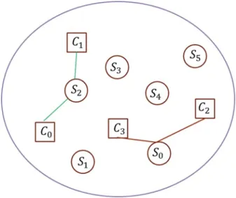
To explain our idea, we firstly define temporary local girth as the local girth of a variable node under the current graph. For PEG-based algorithms, the first edge selection for any variable node is connect with a check node, which has the lowest check node degree under the current graph. Fig. 3.2 illustrates the way the PEG-based algorithms select the first edge for each variables. However, for a variable node, the different choices for its first edge may

Figure 3.2: Original PEG (S3 choose the first edge): Direct select minimum degree survivor. For this case, C0 and C2 are candidates.

lead to different temporary local girths after growing its second edge. More importantly, such manner of connection may lower the maximum achievable cycle length on the other edges of the variable node. This is owing to the subsequent selection of edges will depend on the current selection of an edge. Thus, we prefer to make the temporary local girth which is formed initially for a variable node as large as possible. This way is more likely to make the subsequent temporary local girth large.

Based on this observation, we modify the selection of the first edge for all the variable nodes. The purpose here is to enlarge the values in E. We achieve the purpose by maximizing temporary local girth which is formed initially for a variable node. In this refinement, the modification firstly finds a subset C of check node, which has the lowest check node degree under the current graph. Among the check nodes in this subset, a check node which can result the largest temporary local girth for this variable node is chosen.

Based on the PEG-based algorithm, the procedure of the first edge selection is revised in the above. Note that the step to find the subset C is important. If we omit this step, the output tanner graph might have a non-concentrated check node degree distribution, and the performance of the code will degrade seriously.

3.3

The Second Strategy for Cycle Length-Boosting:

Node-grouping for Selection of The Other Edges

It is easy to figure out that the values in E tend to decrease when the number of edge become larger. The purpose of this strategy is aiming at slowing down the speed of decay in the sequence E. Except for the first edge selection of any variable node, this modification will be applied to the selection of any other edge.

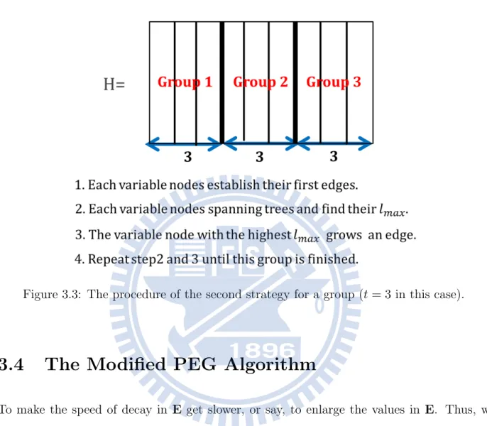
On the other hand, for given code parameters, constructing a parity-check matrix that has the largest girth is a well-known difficult problem. Conventional PEG-based algorithms build up a Tanner graph in a node-by-node manner, that is, all edges incident to a variable node are established before moving to the next variable node. However, such a manner limits the edge growing in a stiff way. This may not be an effective way to maximize the local girth of variable nodes. Here, we provide another possible alternative. Our main idea is to build a Tanner graph in an edge-by-edge manner, i.e., growing edges in a non-deterministic way. The way we establish an edge is to take more variable nodes into consideration simultaneously,

and these variable nodes are regarded as one group. Then, an edge of a node in this group that can maximize the shortest cycle length under the current graph is grown. It is likely to increase the cycle length due to more candidate edges.

Since we take more variable nodes simultaneously into consideration while establishing an edge, so there are some questions, which variable nodes should be taken into consider-ation while an edge is established? Should we take all variable nodes into considerconsider-ation simultaneously? We observe that if high-degree variable nodes growing edges earlier than low-degree variable nodes, these high-degree variable nodes will form longer cycles with larger ACE metric easily. Above behaviour will make those low-degree variable nodes form shorter cycles with smaller ACE metric. To avoid the above observation happens, we propose a Node-grouping approach. Before growing an edge of a tanner graph, we divide all variable nodes into several groups, and variable nodes in the same group are restricted to have the same degree. Every group will have maximal size t. For example, if the number of degree-2 and degree-3 variable nodes are 25 and 15 respectively, and t is 10, then we will have 10 variable nodes in the first and the second group respectively, but only 5 variable nodes are in the third group. The fourth group has 10 variable nodes, and 5 variable nodes are in the fifth group. Note that, this approach also comprises the conventional PEG-based algorithms as a sub-case, i.e, when every group only has one variable node.

After finishing node-grouping, the approach will establish edges group-by-group, the order is from the group with the lowest variable node degree to the group with the highest variable node degree. For a group, before establishing an edge, any variable node vj in this

group will firstly expand their tree to depth l, under the current graph such that Nl_v

j ̸= ∅

but Nl+1_v

j = ∅, or the cardinality of N

l

vj stops increasing but is less than m. Then find a

variable node which has the largest depth l from this group. After that, we grow an edge from this variable node. The procedure repeats growing an edge in such a manner, until all

variable nodes in this group reach their required variable node degree. Fig. 3.3 describes the procedure of the second strategy by using an example.

Figure 3.3: The procedure of the second strategy for a group (t = 3 in this case).

3.4

The Modified PEG Algorithm

To make the speed of decay in E get slower, or say, to enlarge the values in E. Thus, we proposed two strategies above. The first strategy can increase the values in E by modifying the procedure of the first edge selection in the PEG-based algorithm. The second strategy achieves the purpose by modifying the order of edge growing in the PEG-based algorithm. Since the above two mentioned modified strategies all can increase the values in E, and they are applied to the different types of edges, in other words, these two strategies do not conflict with each other. Therefore, we combine them into an algorithm in order to get better performance of the LDPC codes. The initial conditions and the proposed algorithm

is summarized as following:

We set a parameter t as the maximum number of variable nodes in a group. The variable nodes in a group are restricted to have the same degree. We also assume that there are totally w groups without loss of generality. Denoted by Su the uth group. The degree of the

variable node in Siare assumed to be larger or equal to the degree of the nodes in Sk,∀ i ≥ k.

Cycle Length-Boosting PEG algorithm:

• for u = 1 → w

– for each sj ∈ Su (First Edge Connection)

∗ Find the subset C of check nodes, which has the lowest check node degree

under the current graph setting. Among the subset C, the check node candi-date of the first edge which can create the largest cycle length on its second edge is chosen.

– end for

– while at least one variable node not reaches its degree

∗ For each sj ∈ Su whose degree is smaller than dsj, expand a tree from sj up

to depth l under the current graph setting such that Nl_sj ̸= ∅ but Nl+1_sj = ∅, or the cardinality of N_sl_j stops increasing but is less than m.

∗ Let V be a set of comprising the variable nodes that have the largest depth lmax among all tree expansions.

∗ Let Ωj be a subset of check nodes that consists of the check nodes in N lmax

sj

and has the lowest degree.

∗ Randomly choose a variable node si ∈ V , then randomly select a check node

– end

• end

3.5

The Modified Improved PEG Algorithm

In [14], it shows that the improved PEG algorithm is a PEG-based algorithm, which con-siderably enhances the performance at high-SNR region without any degradation in the low SNR performance compare to the original PEG algorithm. In addition, this algorithm is simple and quietly effective in design complexity. Generally speaking, the modification is based on creating a higher degree of connectivity in the tanner graph of the code without sacrificing the girth distribution.

In Section 3.4, a modified version of the original PEG algorithm is presented. From our simulation results, it can be found that considerable improvements in the error floor region relative to the original PEG algorithm. We are also interested in what will the performance be if the strategies are applied to the improved PEG algorithm. Hence, we proposed the algorithm in this section. In this algorithm, the basic structure is similar to the algorithm proposed in Section 3.4, but the complexity is a little higher. The main difference is that the ACE metric is joined in considering in the algorithm. Recall that in our second strategy, we firstly aggregate certain number of variable nodes with the same degree into a group. Then, an edge of a node in this group that can maximize the shortest cycle length under the current graph is grown. However, in this algorithm, we revise the second strategy as stated in the following. After grouping, we expect that, an edge of a variable node in a group that can maximize not only the shortest cycle length, but also the smallest cycle ACE under the current graph is grown. The details of the algorithm is summarized as follow:

nodes in a group are restricted to have the same degree. We also assume that there are totally w groups without loss of generality. Denoted by Su the uth group. The degree of the

variable node in Siare assumed to be larger or equal to the degree of the nodes in Sk,∀ i ≥ k.

Cycle Length-Boosting Improved PEG algorithm:

• for u = 1 → w

– for each sj ∈ Su (First Edge Connection)

∗ Find the subset C of check nodes, which has the lowest check node degree

under the current graph setting. Among the subset C, the check node candi-date of the first edge which can create the largest cycle length on its second edge is chosen.

– end for

– while at least one variable node not reaches its degree

∗ For each sj ∈ Su whose degree is smaller than dsj, expand a tree from sj up

to depth l under the current graph setting such that Nl_s

j ̸= ∅ but N

l+1 sj = ∅,

or the cardinality of Nl

sj stops increasing but is less than m.

∗ Let V be a set of comprising the variable nodes that have the largest depth lmax among all tree expansions.

∗ Let R be a subset of V , which can form cycles with the largest cycle ACE. ∗ Let Ωj be a subset of check nodes that consists of the check nodes in N

lmax

sj

and has the lowest degree.

∗ Randomly choose a variable node si ∈ R. The check node in Ωi that can

– end

• end

3.6

The Other Topics

3.6.1

The First Topic

In this section, we will talk about some topics which related to the PEG-based code construc-tion. In our research, before having the ideas mentioned in previous sections, we had done some attempts, such like change the order of growth edge in order to construct good LDPC codes. Luckily, we found that a scheme among those attempts has good performance in the error floor region. Similar to the second strategy mentioned in Section 3.4, we firstly aggre-gate variable nodes which have the same degree into the same group. Edges are established in a degree-by-degree manner: the order is from low degree group to high degree group. For a group, the first edge of each variable nodes are established, then, the second edge of each variable nodes are established, and the other edges are established by such a way until all the variable nodes reach their required degree. We briefly summarized the algorithm in the following:

Note that dmax is the maximum degree of variable node. Denoted by Sd the dth group.

The other symbols has mentioned in Section 2.2, so we omit here. The Scheme:

• for d = 1 → dmax

– for k = 1→ d

· Expand a tree from sj up to depth l under the current graph setting such that Nl_s j ̸= ∅ but N l+1 sj =∅, or the cardinality of N l

sj stops increasing but

is less than m. Connect the k-th edge of sj with a check node from N l sj

that has the lowest degree.

∗ end for

– end for

• end for

3.6.2

The Second Topic

As we know, before constructing a Tanner graph, conventional PEG based algorithms have to assign the required variable degree to each variable nodes based on the variable node degree distribution. However, in our second strategy, such a way may somehow limits the number of edge candidates while we select an edge in constructing procedure. Thus, we expect that the action to assign the required variable node degree to any variable node can late as much as possible. In order to achieve our purpose, we make some attempts for the given variable node degree distribution. The variable node degree distribution is

λ(x) = 0.47532x2_{+ 0.279537x}3_{+ 0.0348672x}4_{+ 0.108891x}5_{+ 0.101385x}15 _{here. Among these} attempts, one scheme has better BER performance.

This scheme as stated in the following: we aggregate degree-2 variable nodes and degree-3 variable nodes as the first group. The second group comprises degree-4 variable nodes and degree-5 variable nodes. Finally, the last group is composed of degree-15 variable nodes. After grouping, there is still no variable node being assigned variable node degree yet. The order to establish edges is from the first group to the last group, and the way we grow an edge is similar to our second strategy. For a group, while a variable node reach the lowest variable node degree in the group, i.e, for the first group, the lowest degree is two, we assign

this variable node to the lowest variable node degree in the group. When the number of the lowest variable node degree reaches the number we required, each variable nodes in this group are already assigned the variable node degree, since there are only two degrees in one group at most. We complete the procedure of the code construction by such a manner.

Chapter 4

Numerical Results and Discussions

To examine our algorithms, some results in terms of the CLoES, VN-ACES and the BER performance are provided in this chapter. We firstly discussed our two strategies in Section 4.1, and then focus on the algorithms we propose in Section 4.2. The optimal variable node degree distribution λ(x) = 0.47532x2_{+ 0.279537x}3_{+ 0.0348672x}4_{+ 0.108891x}5_{+ 0.101385x}15 which is widely used to construct half-rate LDPC code is adopted as a benchmark, and two codeword lengths, 1008 and 2016, are considered.

4.1

Discussions for The Two Strategies

The strategy for first edges refinement is presented in the Section 3.2. Here, we discuss its results in terms of the CLoES and the BER performance. A simulation result about the use of the first strategy is demonstrated in Fig. 4.1. The line denoted as Original PEG is the BER performance of the original PEG algorithm without using any strategy. The line marked ”Original PEG(the first strategy)” is the BER performance of the original PEG algorithm modified by the first strategy. It can be seen that the BER performance of the modified version of PEG algorithm is better than that of the original PEG algorithm. In addition, the ¯E of the original PEG and the Original PEG(the first strategy) are 12.14 and

12.68 respectively, and the ratio is 4.06 in this case. From above results, we can see that the first strategy is effective. In Fig. 4.2, The line denoted as Improved PEG is the BER performance of the Improved PEG algorithm without using any strategy. The line marked ”Improved PEG(the first strategy)” is the BER performance of the improved PEG algorithm modified by the first strategy. We can see similar improvements depicted in this figure.

2 2.1 2.2 2.3 2.4 2.5 2.6 10−7 10−6 10−5 10−4 E b/N0(dB) BER Original PEG

Original PEG(the first strategy)

Figure 4.1: BERs for the PEG algorithm modified by the first strategy (n=1008 and rate=1/2)

Recall that the second strategy mentioned in Section 3.3. Now we provide some results here. Fig. 4.4 indicates the CLoESs of the original PEG algorithm and the PEG algorithm modified by the second strategy with t = 150. Since no cycle is formed when growing

degree-2 2.1 2.2 2.3 2.4 2.5 2.6 10−7 10−6 10−5 10−4 E b/N0(dB) BER Improved PEG

Improved PEG(the first strategy)

Figure 4.2: BERs for the Improved PEG algorithm modified by the first strategy (n=1008 and rate=1/2)

2 variable nodes for these two algorithms, E(3) _{become the most important sub-sequence in}

CLoES. Thus, Fig. 4.5 demonstrates E(3) _{for these two algorithms. We can observe that}

the values in the CLoES of the modified algorithm generally have larger values than that of the original PEG algorithm, and the most significant effects can be found in E(3). Fig. 4.3 compares the BERs for different parameter t used in the second strategy. The line marked ”Original PEG(the second strategy-n)” is the BER performance of the original PEG algorithm modified by the second strategy with the parameter t equal to n, and the rest lines may be deduced by analogy. We can find that when t is larger, then the better BERs performance it is. Table. 4.1 compares the CLoES for different parameter t we used to

construct codes. It can be seen that when t goes up, then good results can be found for the CLoES of a code. Such results accord with the BERs performance in Fig. 4.3.

2 2.05 2.1 2.15 2.2 2.25 2.3 2.35 2.4 2.45 2.5 10−6 10−5 10−4 E b/N0(dB) BER Original PEG

Original PEG(the second strategy−10) Original PEG(the second strategy−100) Original PEG(the second strategy−150) Original PEG(the second strategy−n)

Figure 4.3: BERs for the PEG algorithm modified by the second strategy with group sizes (n=1008, rate=1/2 and t=10,100,150,n)

4.2

Discussions for The Proposed Algorithms

In this section, several algorithms proposed in Chapter 3 will be discussed in terms of many kind of results. We firstly discuss the modified PEG algorithm proposed in Section 3.4. Taking n = 1008 as an example, we construct several codes by using the PEG, improved PEG and the modified PEG algorithm introduced in Section 3.4. The obtained codes are

Table 4.1: The comparison of CLoES for the second strategy, corresponding to Fig. 4.3 Code P EG Strategy− 10 Strategy − 100 Strategy − 150 Strategy − n

¯

E 12.14 12.14 12.48 12.88 13.08

Ratio – 1.32 3.86 4.10 5.17

named as PEG, IPEG and MPEG,t, respectively. Note that, t is the maximum size of variable nodes in a group.

In Table 4.2, the ¯E’s corresponding to IPEG and MPEG,t with various group size are

presented. Their values show that our algorithm generally generates codes with a longer cycle length than the improved PEG algorithm. Moreover, when t rises, ¯E increases. This

is because that the larger size of a group is, the more edges can be chosen as candidate to maximize cycle length. In addition, for the values in the CLoES of MPEG,t, the increase to decrease cycle length ratio with respect to the CLoES of IPEG are compared with different values of t. When t goes up, it can be seen that a large proportion of cycle length in E also increases. Consequently, the effectiveness of our algorithm is confirmed to a certain extent.

More specifically, the cycle length between variable nodes with different degree and the ACE are compared for IPEG and MPEG,n. The results of the comparisons are summarized in Table 4.4. Here, because both codes have no cycles formed by only the degree-2 variable nodes, their ¯E(2)_{’s are infinite. Additionally, there are cycles formed by only the degree-2} and degree-3 variable nodes in both codes. The average length of those cycles are 26.70 and 30.30 for IPEG and MPEG,n, respectively. Our code shows a longer cycle length in average. In fact, not only for this case, the increments are also observed for other types of cycle. On the other hand, the improved PEG algorithm is known as a good approach to enhance the ACE. However, the resulting ACE shown in Table 4.4 indicates that our code has a better average value. A significant improvement is especially observed for the degree-2 variable nodes. This is interesting since the cycles formed by the degree-2 variable nodes can comprise more variable nodes with higher degree by our algorithm. As a result, it is

0 500 1000 1500 2000 0 10 20 30 40 50 60 70 80 90 100 edge index cycle length CLoES(n=1008) PEG

PEG with the second strategy(t=150)

Figure 4.4: Decay on the CLoESs of the original PEG algorithm and the PEG algorithm modified by the second strategy

expected that our code can have a better BER performance at the high SNR region.

To reveal the BER performances of IPEG and MPEG,n, in our simulation settings, the BPSK modulation for AWGN channels and the SPA are considered. The maximum number of iterations is 100. In Fig. 4.6, for n = 1008, it can be seen that the BER performance of the original PEG code IPEG is improved with the aid of ACE, but our code MPEG,n has an even better performance than IPEG. As reported in literature, this is owing to the longer cycle lengths between low degree variable nodes and hence some harmful structures are largely broken. In addition, for n = 2016, the similar improvements are also observed.

0 50 100 150 200 250 300 350 400 450 500 0 10 20 30 40 50 60 70 80 90 100 edge index cycle length

CLoES for low degree variable nodes(n=1008) PEG

PEG with the second strategy(t=150)

Figure 4.5: Decay on the E(3)_{of the original PEG algorithm and the PEG algorithm modified} by the second strategy

From Table. 4.3 and Table. 4.5, we can see that the increments on cycle length and ACE are similar to the case of n = 1008 and are thus omitted to describe here.

Then, we discuss the modified improved PEG algorithm which proposed in Section 3.5. The codeword length here is 1008. The CLoESs of the improved PEG algorithm and the modified improved PEG algorithm are depicted in Fig. 4.7 and Fig. 4.8. The results of the comparison for ACE and CLoES are also shown in Table 4.6. We can see that the modified improved PEG algorithm always has larger values in CLoES than the improved PEG algorithm. Furthermore, it also indicates that the modified improved PEG algorithm shows

Table 4.2: The comparison of CLoES for various constructions(n = 1008, rate = 1/2), including the improved PEG algorithm and the modified PEG algorithm proposed in Section 3.4

Code IPEG MPEG,10 MPEG,100 MPEG,150 MPEG,300 MPEG,n

¯

E 12.16 12.56 13.07 13.15 13.19 13.28

Ratio – 1.558 3.968 3.995 4.60 4.76

Table 4.3: The comparison of CLoES for various constructions(n = 2016, rate = 1/2), including the improved PEG algorithm and the modified PEG algorithm proposed in Section 3.4

Code IPEG MPEG,20 MPEG,200 MPEG,300 MPEG,600 MPEG,n

¯

E 13.36 14.10 14.58 14.64 14.87 14.82

Ratio – 1.508 4.241 4.448 4.955 5.029

Table 4.4: The Cycle Length and ACE Comparison for PEG, Improved PEG and Modified PEG(t=n) (n = 1008, rate = 1/2) Degree (d) 2 3 4 5 15 Average ¯ E(d) PEG ∞ 26.66 12.88 11.04 6.95 12.14 IPEG ∞ 26.70 12.83 10.68 6.97 12.16 MPEG ∞ 30.30 12.91 11.06 7.44 13.28 ¯ ηd PEG 14.78 15.35 15.36 17.11 14.73 15.20 IPEG 15.98 15.68 15.27 16.10 16.16 15.90 MPEG 17.86 15.71 15.22 16.07 15.54 16.74

Table 4.5: The Cycle Length and ACE Comparison for Improved PEG and Modified PEG(t=n)(n = 2016, rate = 1/2) Degree (d) 2 3 4 5 15 Average ¯ E(d) IPEG ∞ 30.07 14.20 11.57 7.49 13.36 MPEG ∞ 34.77 14.38 12.00 8.11 14.82 ¯ ηd IPEG 17.77 19.67 16.94 17.20 18.14 18.24 MPEG 19.33 19.79 16.82 17.77 18.67 19.14

1.5 1.6 1.8 2 2.2 2.4 2.6 2.8 10−7 10−6 10−5 10−4 E b/N0(dB) BER PEG−2016 Improved PEG−2016 Modified PEG−2016 PEG−1008 Improved PEG−1008 Modified PEG−1008

Figure 4.6: BERs for the modified PEG algorithm (n=2016 and 1008, rate=1/2)

better ACE than the modified PEG algorithm, and their CLoESs are shown similar performs. The performance of this modified algorithm and other algorithms are demonstrated in Fig. 4.9. It can be seen that this algorithm has the best performance among these four algorithms. It is not an unexpected thing, since this algorithm maximize the local girth and ACE metric simultaneously while grows an edge. The complexity of this algorithm is also higher than the other algorithms in Fig. 4.9. In addition, with codeword length 2016, the BERs performance of these algorithms are demonstrated in Fig. 4.10.

Finally, the BER performance of the modified PEG algorithms proposed in Section 3.6 are illustrated in Fig. 4.11. These two algorithms are of better performance compared to the

0 500 1000 1500 2000 0 10 20 30 40 50 60 70 80 90 100 edge index cycle length CLoES(n=1008) Improved PEG

Modified Improved PEG

Figure 4.7: Decay on the CLoESs of the improved PEG algorithm and the modified improved PEG algorithm

original PEG algorithm. Furthermore, these topics are still working, and we guess that these algorithms may gain more improvements by combining the strategies proposed in Chapter 3.

0 50 100 150 200 250 300 350 400 450 500 0 10 20 30 40 50 60 70 80 90 100 edge index cycle length

CLoES for low degree variable nodes(n=1008)

Improved PEG

Modified Improved PEG

Figure 4.8: Decay on the E(3) of the improved PEG algorithm and the modified improved

PEG algorithm

Table 4.6: The Cycle Length and ACE Comparison for Modified PEG and Modified Improved PEG (n=1008, rate=1/2) Degree (d) 2 3 4 5 15 Average ¯ E(d) MPEG ∞ 30.30 12.91 11.06 7.44 13.28 MIPEG ∞ 30.37 12.89 10.98 7.35 13.23 ¯ ηd MPEG 17.86 15.71 15.22 16.07 15.54 16.74 MIPEG 24.33 25.05 24.11 21.13 22.04 23.90

2 2.1 2.2 2.3 2.4 2.5 2.6 2.7 10−7 10−6 10−5 10−4 E b/N0(dB) BER PEG Improved PEG Modified PEG

Modified Improved PEG

1.6 1.65 1.7 1.75 1.8 1.85 1.9 1.95 2 2.05 10−7 10−6 10−5 10−4 E b/N0(dB) BER PEG Improved PEG Modified PEG

Modified Improved PEG

2 2.1 2.2 2.3 2.4 2.5 2.6 10−7 10−6 10−5 10−4 E b/N0(dB) BER Original PEG Proposed in section 3.6.1 Proposed in section 3.6.2

Chapter 5

Conclusion Remarks and Future Work

The PEG algorithm is a good method to construct finite length LDPC codes. However, it has some fundamental weaknesses, such as the improper selection of the first edge and the basic framework of growing edges, which will deteriorate the code structure and degrade the decoding performance. Hence, in this thesis, two strategies are proposed for the PEG-based algorithms. We aim to further enlarge the cycle length formed in the steps of growing edges. One strategy achieves the purpose by refining the selection of the first edge, and the other one changes the original node-by-node construction framework of the PEG algorithm. The new construction framework looks good with the objectives of other optimization, such like ACE metric. Except for the modified PEG algorithm, the modified algorithm based on the improved PEG algorithm is also a successful example proposed in Section 3.5. It is observed that our proposed algorithms can improve the ACE and the BER performance. With the proposed informative sequence called CLoES, a detailed inspection for the codes constructed by our algorithms is also made. The obtained results confirm that our strategies can effectively increase the cycle lengths formed in the Tanner graph.

In addition, several issues can be further studied. The first one is that the algorithms mentioned in Section 3.6 may be further improved by combining our strategies into them-selves. Another one is that the new construction framework may try to optimize more

objec-tives simultaneously, for example, girth, ACE, number of cycles and even the objecobjec-tives not mentioned in the thesis. Other than these two, the CLoES provides useful viewpoints for improving the performance of the PEG-based codes, thus it can be worthy of further study.

Bibliography

[1] R. G. Gallager, “Low-density parity-check codes,” IRE Trans. Inf. Theory, vol. 8, pp. 21-28, Jan. 1962.

[2] C. Y. Di et al., “Finite-length analysis of low-density parity-check codes on the binary erasure channel,” IEEE Trans. Inf. Theory , vol. 48, pp. 1570-1579, June 2002.

[3] T. J. Richardson, “Error floors of LDPC codes”, in Proc. 41st Annual Allerton Conf.

on Commun., Control and Computing, Monticello, IL, USA, Oct. 2003, pp. 1426-1435.

[4] L. Dolecek, Z. Zhang, V. Anantharam, M. J. Wainwright, and B. Nikolic, “Analysis of absorbing sets for array-based LDPC codes,” in Proc. IEEE International Conf.

Commun. , Glasgow, Scotland, June 2007, pp. 6261- 6268.

[5] T. Tian, C. Jones, J. D. Villasenor, and R. D. Wesel, “Selective avoidance of cycles in irregular LDPC code construction,” IEEE Trans. Commun., vol. 52, pp. 1242-1247, Aug. 2004.

[6] X. Y. Hu, E. Eleftheriou, and D. M. Arnold, “Regular and irregular progressive edge-growth Tanner graphs,” IEEE Trans. Inf. Theory , vol. 51, no. 1, pp. 386-398, Jan. 2005.

[7] G. Richter and A. Hof, “On a construction method of irregular LDPC codes without small stopping sets,” in Proc. IEEE ICC’06. Istanbul, Turkey, 11-15 Jun. 2006, pp. 1119-1124.

[8] X. Jiao, J. Mu, J. Song, and L. Zhou, “Eliminating small stopping sets in irregular low-density parity-check codes,” IEEE Comm. Lett., vol.13, no. 6, pp. 435437, June 2009.

[9] G. Richter, “Construction of completely regular LDPC codes with large

girth,” in Proc. ETH Zurich 2003 Winter School on Coding

andInfor-mation Theory, Ascona, Switzerland, Feb. 2003. Available [Online] at http://www.isi.ee.ethz.ch/winterschool/docs/richter.pdf.

[10] E. Psota, and L. Perez, “Iterative construction of regular LDPC codes from independent tree-based minimum distance bounds,“ IEEE Comm. Letts., vol. 15, no. 3, pp. 334-336, Mar. 2011.

[11] Him Chen and Zhigang Cao, “A Modified PEG Algorithm for Construction of LDPC Codes with Strictly Concentrated Check-Node Degree Distributions,” Wireless

Communications and Networking Conference, 2007.WCNC 2007. IEEE, On page(s): 564

-568.

[12] G. Richter, “An improvement of the PEG algorithm for LDPC codes in the waterfall region,” in International Conference on Computer as a tool (EUROCON), Belgrade, Serbia and Montenegro, Nov. 2005.

[13] Lei Xiong, Dongping Yao and Yimeng Wu, “A modified PEG algorithm for construction of LDPC codes with Polynomial of Cycle,” in Proc. 3rd IEEE International Symposium

on Microwave, Antenna, Propagation and EMC Tech. for Wireless Commun., Beijing,

[14] H. Xiao and A. H. Banihashemi, “Improved progressive-edge-growth (PEG) construc-tion of irregular LDPC codes,” IEEE Comm. Letts., vol. 8, pp. 715-717, Dec. 2004. [15] Y. Mao and A. Banihashemi, “A heuristic search for good low-density parity-check codes

at short block lengths,” in Proc. IEEE Int. Conf. Comm., Helsinki, Finland, pp.41-44, Jun. 2001.

[16] T. Richardson, M. Shokrollahi, and R. Urbanke, “Design of capacity-approaching ir-regular low-density parity-check codes,” IEEE Trans. Inf. Theory, vol. 47, no. 2, pp. 619-637, Feb. 2001.

[17] D. Vukobratovic, A. Djurendic, and V. Senk, “ACE spectrum of LDPC codes and generalized ACE design,” in Proc. IEEE ICC’07, Glasgow, Scotland, 24-28 Jun. 2007, pp. 665-670.