The Discrete Fractional Cosine and Sine Transforms
Soo-Chang Pei, Fellow, IEEE, and Min-Hung Yeh
Abstract—This paper is concerned with the definitions of the
discrete fractional cosine transform (DFRCT) and the discrete fractional sine transform (DFRST). The definitions of DFRCT and DFRST are based on the eigen decomposition of DCT and DST kernels. This is the same idea as that of the discrete fractional Fourier transform (DFRFT); the eigenvalue and eigenvector relationships between the DFRCT, DFRST, and DFRFT can be established. The computations of DFRFT for even or odd signals can be planted into the half-size DFRCT and DFRST calculations. This will reduce the computational load of the DFRFT by about one half.
Index Terms—Discrete fractional cosine transform, discrete
fractional Fourier transform, discrete fractional sine transform.
I. INTRODUCTION
T
HE FRACTIONAL Fourier transform (FRFT) is a gener-alized Fourier transform [1]–[5]; in addition, the FRFT is a special case of the more general linear canonical transform [6], and it provides a tool to compute the mixed time and fre-quency components of signals. The interpretation of the FRFT is a rotation of signals in the time–frequency plane. Because of the importance of the FRFT, the discrete fractional Fourier transform (DFRFT) has also become an important issue recently [7]–[11]. In the development of the DFRFT, it has been consid-ered to be a linear weighted summation of the signal and spec-trum [7]. Unfortunately, such a method cannot have the outputs that are similar to the continuous case [8]. It will work very similarly to the original transform or the identity operation and lose the important characteristics of fractionalization. We have found that the DFRFT with discrete Hermite eigenvectors and an appropriate eigenvalue assignment rule satisfy all the desir-able properties and can have similar results as those of contin-uous FRFT [9]. The authors further improved this type of dis-crete fractional Fourier transform (DFRFT) by modifying their eigenvectors more closely to the continuous Hermite eigenvec-tors [10]. This eigendecomposition method for the DFRFT has been consolidated in [11]. Moreover, the eigendecomposition methods for the DFRFT have been used as a tool in many appli-cations [12], [13].Orthogonal transforms are widely used in signal analysis and image compression [14]. Besides the DFRFT, several fractional signal transforms have also been developed in recent
Manuscript received October 2, 2000; revised February 16, 2001. The asso-ciate editor coordinating the review of this paper and approving it for publication was Dr. Xiang-Gen Xia.
S.-C. Pei is with the Department of Electrical Engineering, National Taiwan University, Taipei, Taiwan, R.O.C. (e-mail: [email protected]).
M.-H. Yeh is with the Department of Electronic Engineering, Na-tional I-Lan Institute of Technology, I-Lan, Taiwan, R.O.C. (e-mail: [email protected]).
Publisher Item Identifier S 1053-587X(01)03887-9.
documents, such as the discrete fractional Hartley transform [13] and the discrete fractional Hadamard transform [15]. Unfortunately, the fractional versions of the discrete cosine transform (DCT) and the discrete sine transform (DST) are still absent. The purpose of this paper is to develop the generalized versions of the DCT, DST, DFRCT and DFRST. This paper is organized as follows. In Section II, preliminaries about the DCT, DST, and DFRFT are given. Then, the eigenvectors and eigenvalues of the DCT and DST are studied in Section III. In Section IV, we develop the DFRCT and DFRST. Moreover, the steps for computing the DFRCT and DFRST kernel matrices are also summarized. The properties of DFRCT and DFRST are discussed in Section V, and the final conclusions are made in Section VI.
II. PRELIMINARY A. Four Types of DCT Kernel Matrices
The definitions of DCT and DST kernel matrices have been well reviewed in [16]. We will quote them here for our further discussion. In [16], four types of DCT kernel matrices are pre-sented, and they are shown as follows.
• DCT-I (1) for . • DCT-II (2) for . • DCT-III (3) for . • DCT-IV (4) for .
and in the above four definitions are defined as and
others.
(5)
B. Four Types of DST Kernel Matrices
Similar to the DCT case, the DST also has four definitions in [16]. The four types of DST kernel are shown as follows.
• DST-I (6) for . • DST-II (7) for . • DST-III (8) for . • DST-IV (9) for .
and in the above four definitions are the same as those in (5). The DCT-I and DST-I kernels have symmetric structures and are periodic with period 2. The periodicity means that re-peated application of DCT-I and DST-I would give the orig-inal sequence. DCT-IV is the same as DCT-I for symmetry and periodicity, but DCT-II and DCT-III operators are the forward
and inverse transform pair of each other and are nonperiodic. Here, DCT-I and DST-I will be chosen and used in developing DFRCT and DFRST, as shown in (10) and (11) at the bottom of the page.
C. Discrete Fractional Fourier Transform
The continuous FRFT performs a rotation of signal in the time–frequency plane, and the conventional Fourier transform is a rotation of signal [1]. Similar to the continuous notation, the DFT can be regarded as a rotation for discrete signals [10]. The DFT kernel is defined in the following way for energy preservation.
..
. . .. ...
(12)
where . The DFRFT performs any angle
ro-tation for discrete signals [9], [10]. Several DFRFTs have been developed [7], [9], [10]. It has been proved that the DFRFT in [7] cannot have similar results [8]. The DFRFT concerned in this paper is the eigendecomposition-based method in [9] and [10]. The methods in [9] and [10] use the DFT Hermite eigenvectors to construct the DFRFT kernel matrix. It has been shown that
..
. ... . .. ... ... (10)
..
TABLE I
EIGENVALUEMULTIPLICITIES OF THEDFT KERNELMATRICES
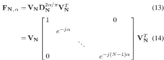
the methods in [9] and [10] can have similar outputs as the con-tinuous results. In [9] and [10], the -point DFRFT kernel is computed as
(13)
. .. (14)
where , is the th order DFT
Her-mite eigenvector, and indicates the rotation angle of transform in the time–frequency plane. When , is an identity operator. If , the DFRFT becomes the conventional DFT. Several methods for finding the th-order DFT Hermite eigenvectors have been proposed in [9] and [10].
III. EIGENVECTORS ANDEIGENVALUES OFDCTANDDST KERNELMATRICES
The eigenvectors and eigenvalues of the DFT kernel matrix are well studied in [17]–[19], and it is very helpful to develop the DFRFT. However, the eigenvectors and eigenvalues of DCT and DST kernel matrices are still absent in the current documents. In this section, we will study the eigenvectors and eigenvalues of DCT and DST kernel matrices. This will help us to develop the DFRCT and DFRST.
Proposition 1: The DFT kernel matrix has only four distinct
eigenvalues— —and its multiplicities are
sum-marized in Table I. Proof: See [17].
Because the DFT has only four distinct eigenvalues, the DFT eigenvectors will constitute four eigenspaces. It is trivial to find that any vector spanned by the DFT eigenvectors corresponding to the same eigenvalue is still a DFT eigenvector. Therefore, there exist infinite eigenvectors for the DFT kernel matrix. The multiplicities of DFT eigenvalues are just the dimensions of eigenspaces.
Proposition 2: All the DFT eigenvectors are even or odd. The even eigenvectors are with the eigenvalues 1 or 1; in ad-dition, the odd eigenvectors correspond to the eigenvalues or
.
TABLE II
EIGENVALUEMULTIPLICITIES OF THEDCT-I KERNELMATRICES
Proof: See [17].
The above proposition is very important for the development of DFRCT and DFRST; therefore, we review it here. In the fol-lowing discussion, we will study the eigenvalues and eigenvec-tors for the DCT and the DST and establish the relationships with the conventional DFT.
Proposition 3: The DCT-I and DST-I eigenvectors can be attained from the DFT eigenvectors.
1) If is an
even eigenvector of the -point DFT kernel
ma-trix. ( ). Then
(15) will be an eigenvector of the -point DCT-I kernel ma-trix, where is the corresponding eigenvalue
(16)
2) If , , ,
is an odd eigenvector of the -point DFT kernel
matrix. ( ). Then
(17) will be an eigenvector of the -point DST-I kernel ma-trix, where is the corresponding value
(18) Proof: See the Appendix.
For the odd DFT eigenvectors, because is equal to or , the DST-I eigenvalue will be equal to 1 or 1. From the above proposition, we know that the DCT-I and DST-I kernel matrices have the eigenvalues 1 and . Do there exist other eigenvalues for DCT-I and DST-I besides 1 and ? We will show that the DCT-I and DST-I kernel matrices are with only these two eigenvalues in the following proposition.
Proposition 4: The eigenvalues of DCT-I and DST-I kernel matrices are only 1 and 1. Their multiplicities are shown in Tables II and III, respectively.
TABLE III
EIGENVALUEMULTIPLICITIES OF THEDST-I KERNELMATRICES
Proof: For the DCT-I case, the following results can be derived by Proposition 3:
the -point
DCT-I eigenvectors the -point
DFT even eigenvectors if is even
if is odd
where indicates the multiplicity of an eigenvalue.
Regard-less of is even or odd, the sum of and are both
equal to . Thus, the DCT-I eigenvectors obtained from the DFT even eigenvectors can result in a full-rank DCT-I kernel matrix. All the DCT-I eigenvectors can be obtained from the DFT even eigenvectors. Therefore, Table II is attained.
The results in the DST-I case can be proved in the same way so that Table III can be obtained.
Proposition 5: The orthogonality in DCT-I and DST-I eigen-vectors can be inherited from that in DFT eigeneigen-vectors.
1) If and ( ) are both the even and orthogonal
DFT eigenvectors, the DCT-I eigenvectors and will also be orthogonal.
2) If and ( ) are both the odd and orthogonal
DFT eigenvectors, the DST-I eigenvectors and will also be orthogonal.
Proof: We can compute the inner product of and to check the orthogonality. Using the definitions of and , the following equations could be obtained:
The orthogonality between and can be proved in the same way.
Proposition 5 tells us that the DFT orthogonal eigenvectors can be used to generate the DCT-I and DST-I orthogonal eigen-vectors.
IV. DEVELOPMENT OF THEDISCRETEFRACTIONALCOSINE ANDSINETRANSFORMS
From the previous discussions, we know that all the DFT, DCT, and DST transform kernels have infinite eigenvectors. In [9], [10], and [18], a novel matrix is introduced to compute the real-value and complete set of DFT eigenvectors very el-egantly. This particular set of eigenvectors constitutes the dis-crete analogs of the continuous Hermite–Gaussian functions. We call it the DFT Hermite eigenvectors [9], [10], [18]. Because the DFRFT defined with these DFT Hermite eigenvectors can have similar output as continuous FRFT and will have the prop-erties of unitarity, additivity, and reversibility, the DFT Hermite eigenvectors will be used in developing DFRCT and DFRST as reasonable choices. The eigenvector will have the eigenvalue ( is even) for the DFRCT kernel matrix. Such an assign-ment rule will result in a DCT kernel for . Similar to the DFRFT, the -point DFRCT kernel can be defined as
(19)
. .. (20)
where . is the DCT-I eigenvector
obtained from the th-order DFT Hermite eigenvector by (15).
While , the DFRCT will become the conventional
DCT-I. When , is an identity matrix. The steps
for constructing the -point DFRCT kernel with angular pa-rameter are summarized as follows.
• Step 1) Compute the -point DFT Hermite even
eigen-vectors. .
• Step 2) Use (15) to compute the DCT-I eigenvectors from the DFT Hermite even eigenvectors.
• Step 3) Determine the DFRCT transform kernel by the following equation:
(21)
where . is the DCT-I
eigen-vector obtained from the th-order DFT Hermite eigen-vector by (15).
Similar to the DFRCT case, the development of DFRST is also based on the DFRFT. The eigenvector ( is odd) is assigned to the eigenvalue . Thus, the -point DFRST kernel is defined as
(22)
. .. (23)
where . is the DST-I eigenvector
The above DFRST kernel matrix will be reduced to a DST-I kernel matrix for , and it will become an identity matrix for . The steps for computing the -point DFRST kernel with parameter are summarized as follows:
• Step 1) Compute the -point DFT Hermite odd
eigen-vectors. .
• Step 2) Use (17) to compute the DST-I eigenvectors from the DFT Hermite odd eigenvectors.
• Step 3) Determine the DFRST transform kernel
(24)
where . is the DST-I
eigen-vector obtained from the th-order DFT Hermite eigen-vector by (17).
Since no fast algorithm has been developed for exactly computing the DFRFT, DFRCT, and DFRST transform ma-trix products, their computation would take order
complexity by an ordinary matrix multiplication [10]. An
approximate fast algorithm has been described in
[8] for fast DFRFT computation.
V. PROPERTIES OFDFRCTANDDFRST A. Properties of DFRCT and DFRST
The DFRCT and DFRST developed in this paper are not the same as the conventional DCT and DST with real values in the kernel matrices. Recently, some types of fractional cosine and sine transforms have been derived by taking the real part and imaginary part of the DFRFT kernel [20], although these frac-tional transforms are real and can be implemented with inco-herent light [21]–[23]. However, the angle additivity will not exist for these transforms, and more importantly, they do not have simple inverse transforms.
Because the DFRCT and DFRST are developed with a similar method as the DFRFT, the properties of the DFRCT and the DFRST are inherited from the DFRFT.
• Unitarity:
Similar to the DFRFT, the DFRCT and DFRST are both unitary
(25) (26) • Angle additivity:
Both the DFRCT and DFRST can preserve the angle additive property as the DFRFT
(27) (28) • Periodicity:
The DFRFT is periodic with period , but the DFRCT and the DFRST are periodic with period
(29) (30)
• Symmetric:
Both the DFRCT and DFRST kernel matrices are sym-metric
(31) (32)
B. Relationship Between the DFRCT, DFRST, and DFRFT In this section, we will establish the relationship between the outputs of the DFRCT, the DFRST, and the DFRFT. Moreover, we will show that the DFRFT can be computed by a smaller transform kernel with the help of the DFRCT or the DFRST for the even or odd signal.
Proposition 6: For an even signal of length , ,
, where the DFRFT
output is , , ,
the DFRCT of signal of length , ,
will be equal to
(33)
For an odd signal of length , ,
, , if its DFRFT output is , , ,
, , , the DFRST of signal
of length , , will be equal
to
(34) Proof: The proof can be directly attained from the defini-tions of the DFRCT and the DFRST.
Proposition 6 tells us that the DFRFT of an even or odd signal can be computed by a smaller-size transform kernel of the DFRCT and the DFRST. In [13], the DFT kernel matrix is decomposed into its real and imaginary parts as below. Here, we will apply the notation for dealing with the input signal with even length
(35) where
(36)
(37) Moreover, the DFRFT can be proved and computed through the
fractional power of and in [13]
(38) From [13], we know that the is for the DFRFT compu-tation of an even signal, and is for the DFRST computation of an odd signal. The construction of matrix is from the DFT Hermite even vectors, and is from the other odd vectors [13]. However, the DFRCT and the DFRST are from the truncated and scaled DFT eigenvectors by (15) and (17). Be-cause a general signal can be decomposed into an even and an odd signals, the DFRFT for a discrete signal with even length
Fig. 1. Block diagram for the DFRFT computation by DFRGT and DFRST.
can be computed by and . In Fig. 1, a
dis-crete signal with even length is decomposed into even and odd parts. The even part of signal is computed by the DFRCT and the odd part by the DFRST. Then, the outputs of DFRCT and DFRST are merged to get the desired DFRFT. No matter whether it is the the even or the odd part, a preprocessing (trun-cation) and postprocessing (extension) are required in order to get the desired length. The even and odd parts of signal can be obtained by the following equations:
(39)
(40)
It is easy to check that the entries in are zeros for the two
cases: and . Before the DFRCT and DFRST
computation, a preprocessing (the even and half truncation) is required to shorten the length of the signal. The even and odd half truncations in Fig. 1 are defined as
Even truncation
for (41)
Odd truncation
for (42)
After the truncation, the length of the even part is ( ), and the odd part becomes ( ). The odd truncation is with a unit shift of . After the DFRCT and DFRST computations, the even and odd extensions are required to result in the DFRFT with length
Even Extension
(43) Odd Extension
(44)
In Fig. 1, the phase factor in merging the odd extension comes from (38). The upper part of Fig. 1 is for computing
; the lower part is for . If , the phase
factor becomes , and the and compute
the real and imaginary parts of the conventional DFT, respec-tively. Thus, the computation of the DFRFT can be computed by smaller size of the DFRCT and DFRST transform kernels be-cause the computational loads of the DFRFT, the DFRCT, and the DFRST are all . It is reasonable to assume that the -point transform computations of the DFRFT, the DFRCT and the DFRST need ( ) operations, where indicates a constant for the DFRCT and DFRST computations. The scheme in Fig. 1
will need operations. This can reduce
the computational load of DFRFT about one half.
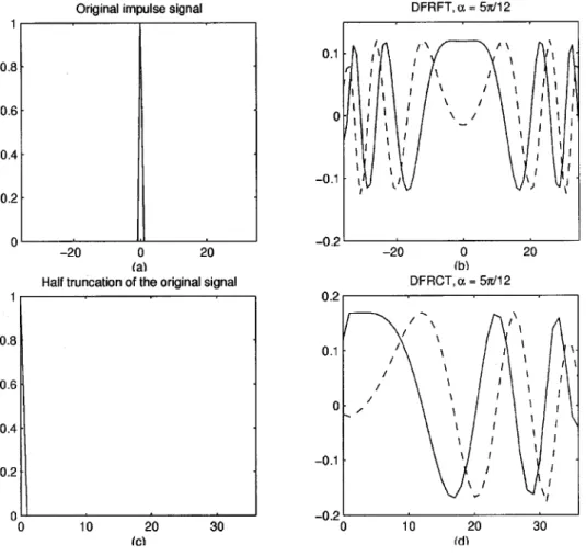
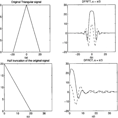
Example 1: In this example, we deal with the DFRCT and DFRFT results for an impulse signal with length 72. Fig. 2(a) shows the original impulse signal, whose DFRFT with angular parameter is shown in Fig. 2(b). The even half trunca-tion of the impulse signal is drawn in Fig. 2(c). Fig. 2(d) is the DFRCT output of the truncated signal. We can observe that the DFRCT result is equal to the positive part of the DFRFT result, but the first and last entries of the DFRCT are scaled by . Example 2: In this example, we further consider the DFRCT and DFRFT results for a triangular signal
. (45)
The triangular signal with length 72 is plotted in Fig. 3(a). We then compute the DFRFT of and draw the output [see Fig. 3(b)]. Fig. 3(c) shows the even truncation of . We com-pute the DFRCT for the truncated triangular signal and show the output in Fig. 3(d). Comparing the results in Fig. 3(b) and (d), we can observe that the first and last entries of DFRCT are
scaled by .
VI. CONCLUSIONS
In this paper, the definitions of discrete fractional cosine and sine transforms (DFRCT and DFRST) have been presented. First, the eigenvalues and eigenvectors of the DCT and DST are investigated. The eigenvalue and eigenvector relationships between the DFRCT, DFRST, and DFRFT are established. Then, the eigendecompositions of the transform matrices are used to define the DFRCT and DFRST kernel matrices. The computations of the DFRFT for even or odd signals can be planted into the DFRCT and DFRST calculations. Moreover, a signal can be decomposed into even and odd signals. With the help of the DFRCT and DFRST, a smaller size of kernel matrix is used for DFRFT computation. This can reduce the computational load of the DFRFT.
APPENDIX
To begin with, we will prove the DCT-I case. It is assumed that is the ( )-point even DFT eigenvector corresponding to the eigenvalue . , or
Fig. 2. Impulse signal and its transform results in Example 1.
Using the definition of the DFT in (12), the following equa-tion can be obtained.
.. . ... ... ... ... .. . ... ... ... ... .. . .. . .. . .. . (A.1)
where . We can check the entries on both sides
Fig. 3. Triangular signalx(n) and its transform results in Example 2.
for . Therefore
(A.2)
Thefollowing equation can be easily attained asin (A.3),shown at the bottom of the page. Equation (A.3) can be written as
(A.4) Therefore, is also the eigenvalue of the DCT-I kernel matrix,
and , is the eigenvector
of DCT-I.
..
. ... ... . .. ... ...
..
.. . .. . ... . .. ... ... .. . (A.7)
Now, we will prove the DST-I case. It is assumed that is the ( )-point odd DFT eigenvector corresponding to the
eigenvalue . or
Using the DFT definition in (12) can lead to the
.. . ... ... ... ... .. . ... ... ... ... .. . .. . .. . .. . (A.5)
where . We can check the entries on the
left side of (A.5).
for . Therefore
(A.6)
The following equation can be easily obtained as in (A.7), shown at the top of the page. Equation (A.7) can be written as
(A.8)
Therefore, is a DST-I eigenvector,
and is its corresponding eigenvalue. If is a normalized
DFT eigenvector, will also be a
nor-malized DST-I eigenvector. The proof of Proposition 3 is com-pleted.
REFERENCES
[1] L. B. Almeida, “The fractional Fourier transform and time-frequency representation,” IEEE Trans. Signal Processing, vol. 42, pp. 3084–3091, Nov. 1994.
[2] A. C. McBride and F. H. Kerr, “On Namias’ fractional Fourier trans-forms,” IMA J. Appl. Math., vol. 39, pp. 159–175, 1987.
[3] V. Namias, “The fractional order Fourier transform and its application to quantum mechanics,” J. Inst. Math. Applicat., vol. 25, pp. 241–265, 1980.
[4] N. Wiener, “Hermitian polynomials and Fourier analysis,” J. Math.
[5] E. U. Condon, “Immersion of the Fourier transform in a continuous group of functional transformations,” Proc. Nat. Acad. Sci., vol. 23, pp. 158–164, 1937.
[6] K. B. Wolf, “Construction and properties of canonical transform,” in
Integral Transforms in Science and Engineering. New York: Gordon and Breech, 1979, ch. 9.
[7] B. Santhanam and J. H. McClellan, “The discrete rotational Fourier transform,” IEEE Trans. Signal Processing, vol. 42, pp. 994–998, Apr. 1996.
[8] H. M. Ozaktas, O. Arikan, M. A. Kutay, and G. Bozdagi, “Digital computation of the fractional Fourier transform,” IEEE Trans. Signal
Process., vol. 44, pp. 2141–2150, Sept. 1996.
[9] S. C. Pei and M. H. Yeh, “Improved discrete fractional Fourier trans-form,” Opt. Lett., vol. 22, pp. 1047–1049, July 15, 1997.
[10] S. C. Pei, M. H. Yeh, and C. C. Tseng, “Discrete fractional Fourier trans-form based on orthogonal projection,” IEEE Trans. Signal Processing, vol. 47, pp. 1335–1348, May 1999.
[11] C. Candan, M. A. Kutay, and H. M. Ozaktas, “The discrete fractional Fourier transform,” IEEE Trans. Signal Processing, vol. 48, pp. 1329–1337, May 2000.
[12] S. C. Pei and M. H. Yeh, “Discrete fractional Hilbert transform,” in Proc.
IEEE Int. Symp. Circuits Syst., June 1998, pp. 506–509.
[13] S. C. Pei, C. C. Tseng, M. H. Yeh, and J. J. Shyu, “Discrete fractional Hartley and Fourier transforms,” IEEE Trans. Circuit Syst. II, vol. 45, pp. 665–675, Apr. 1998.
[14] A. K. Jain, Fundamentals of Digital Image Processing. Englewood Cliffs, NJ: Prentice-Hall, 1989.
[15] S. C. Pei and M. H. Yeh, “Discrete fractional Hadamard transform,” in
Proc. IEEE Int. Symp. Circuits Syst., June 1999, pp. 1485–1488.
[16] Z. Wang, “Fast algorithm for the discreteW transform and for the discrete Fourier transform,” IEEE Trans. Acoust., Speech, Signal
Processing, vol. ASSP-32, pp. 803–816, Aug. 1984.
[17] J. H. McClellan and T. W. Parks, “Eigenvalue and eigenvector decom-position of the discrete Fourier transform,” IEEE Trans. Audio
Electroa-coust., vol. AU-20, pp. 66–74, Mar. 1972.
[18] B. W. Dickinson and K. Steiglitz, “Eigenvectors and functions of the discrete Fourier transform,” IEEE Trans. Acoust., Speech, Signal
Pro-cessing, vol. ASSP-30, pp. 25–31, Feb. 1982.
[19] G. Cincotti, F. Gori, and M. Santarsiero, “Generalized self-Fourier func-tions,” J. Phys., vol. 25, pp. 1191–1194, 1992.
[20] A. W. Lohmann, D. Mendlovic, Z. Zalevsky, and R. G. Dorsch, “Some important fractional transforms for signal processing,” Opt. Commun., vol. 126, pp. 18–20, 1996.
[21] D. Mendlovic, Z. Zalevsky, N. Konforti, R. G. Dorsch, and A. W. Lohmann, “Incoherent fractional Fourier transform and its optical implementation,” Appl. Opt., vol. 34, pp. 7615–7620, Nov. 1995. [22] A. V. Lohmann, D. Mendlovic, and Z. Zalevsky, “Fractional transforms
in optics,” in Progress in Optics, E. Wolf, Ed. Amsterdam, The Nether-lands: North-Holland, 1998, vol. 38, pp. 263–342.
[23] H. M. Ozaktas, M. A. Kutay, and D. Mendlovic, “Introduction to the fractional Fourier transform and its applications,” in Advances
in Imaging and Electron Physics, P. W. Hawkes, Ed. San Diego: Academic, 1999, vol. 106, pp. 239–291.
Soo-Chang Pei (F’00) was born in Soo-Auo, Taiwan,
R.O.C., in 1949. He received the B.S.E.E. from Na-tional Taiwan University (NTU), Taipei, in 1970 and the M.S.E.E. and Ph.D. degrees from the University of California, Santa Barbara (UCSB), in 1972 and 1975, respectively.
He was an Engineering Officer with the Chinese Navy Shipyard from 1970 to 1971. From 1971 to 1975, he was a Research Assistant at UCSB. He was Professor and Chairman in the Electrical Engineering Department, Tatung Institute of Tech-nology and NTU, from 1981 to 1983 and 1995 to 1998, respectively. Presently, he is a Professor with the Electrical Engineering Department, NTU. His research interests include digital signal processing, image processing, optical information processing, and laser holography.
Dr. Pei received the National Sun Yet-Sen Academic Achievement Award in Engineering in 1984, the Distinguished Research Award from the National Sci-ence Council from 1990 to 1998, the Outstanding Electrical Engineering Pro-fessor Award from the Chinese Institute of Electrical Engineering in 1998, and the Academic Achievement Award in Engineering from the Ministry of Edu-cation in 1998. He was President of the Chinese Image Processing and Pattern Recognition Society in Taiwan from 1996 to 1998 and is a member of Eta Kappa Nu and the Optical Society of America.
Min-Hung Yeh was born in Taipei, Taiwan,
R.O.C., in 1964. He received the B.S. degree in computer engineering from the National Chiao-Tung University, Hsinchu, Taiwan, in 1987. He then received the M.S. degree in computer science and information engineering in 1992 and the Ph.D. degree in electrical engineering in 1997, both from the National Taiwan University, Taipei.
From 1997 to 1999, he was an Assistant Professor with the Department of Computer Information Sci-ence, Aletheia University, Tamsui, Taipei. He is cur-rently an Assistant Professor with the Department of Electronic Engineering, National I-Lan Institute of Technology, I-Lan, Taiwan. His main research in-terests are in the fractional Fourier transform, time–frequency analysis, and wavelets.