設限資料下分量迴歸模型分析之文獻回顧

國立交通大學

統計學研究所

碩士論文

設限資料下分量迴歸模型分析之

文獻回顧

Quantile Regression Analysis

based on Censored Data

A Literature Review

研 究 生: 林欣穎

指導教授: 王維菁 博士

i

設限資料下分量迴歸模型分析之

文獻回顧

Quantile Regression Analysis based on Censored Data

A Literature Review

研 究 生: 林欣穎 Student: Hsin-Ying Lin

指導教授: 王維菁 博士

Advisor: Dr. Wei-Jing Wang

國 立 交 通 大 學

統 計 學 研 究 所

碩 士 論 文

A Thesis

Submitted to Institute of Statistics

College of Science

National Chiao Tung University

in Partial Fulfillment of the Requirements

for the Degree of

Master

in

Statistics

May 2011

Hsinchu, Taiwan, Republic of China

ii

設限資料下分量迴歸模型分析之

文獻回顧

研 究 生: 林欣穎 指導教授: 王維菁 博士

國立交通大學理學院

統計學研究所

摘要

在此論文中，我們回顧分量迴歸模型的重要文獻。首先，我們介

紹在沒有變數之完整資料下，估計分量的推論技巧，藉此了解分量的

幾何結構和分析上問題的困難處。接著，我們引進變數的影響和討論

不同的估計程序，並提供幾何上的解釋意義。最後，我們加入設限的

影響並且討論幾種修正的估計方法。我們提供系統化的架構，讓讀者

透過推論方法基本的建構原則，對分量迴歸模型有初步的了解。

關鍵詞: 設限, 分量迴歸模型

iii

Quantile Regression Analysis

based on Censored Data

A Literature Review

Student:

Hsin-Ying

Lin

Advisor:

Dr.

Wei-Jing

Wang

Institute of Statistics

National Chiao Tung University

Hsinchu, Taiwan

Abstract

In the thesis, we review important literature on quantile regression

models for survival data. First, we introduce the inference techniques for

estimating a quantile based on complete data without covariates. This

allows us to see the geometric structure and analytical difficulty of the

problem. Then we include the effect of covariates and discuss different

estimation procedures. Geometric explanations are also provided. Finally

the effect of censoring is incorporated and we discuss several approaches

of modification. We aim to provide a systematic framework which allows

the readers to understand the quantile regression model from fundamental

inference principles.

iv

致 謝

隨著此篇論文的完成，我的學生生涯即進入尾聲，將要踏出校園，

邁向未知的職場生活。在碩士這兩年的求學生涯，不僅學到統計方面

的專業知識，更體會到人生中酸甜苦辣的滋味，我所經歷的每件事、

所相處的每個人，都充實、豐盛了我的生命。

首先，最想感謝的是我的指導教授-王維菁老師，每次討論完論

文後，對於老師的佩服又更加深一層。遵循老師的指導，我體驗到大

體架構的重要性，若不了解文章整體結構為何，鑽研枝微末節也只是

徒然，不僅點出我一直以來的問題，也訓練我先從大局上著手。另一

個重要的是，大膽猜測並用自己的話語表達理解的事物，若沒辦法將

所讀加以理解、吸收並用自己的意見表達出來，那不過是抄襲他人的

想法罷了。在老師身邊，不只學到做學問的態度，也體悟到做人處事

的道理，比起研究，我想這是更重要的，謝謝老師這一年來的教導。

接著，我要感謝的是郭姐和每一位教授熱切的關心和不時的小叮

嚀，讓我在所上的日子備感溫馨；還有共同努力的同學們，在沮喪時

帶來鼓勵、在開心時一同享樂、在作業堆裡攜手共度難關，謝謝你們。

林欣穎 僅誌

中華民國 一百年夏

于交通大學統計學研究所

v

Contents

1. Introduction………..1

1.1 Different types of regression models………...1

1.2 Examples of quantile regression models……….2

1.3 Comparison with other regression models………..5

2. Inference without Censoring………...6

2.1 Inference based on homogeneous data………....6

2.2 Inference based on quantile regression analysis………..7

2.3 Numerical algorithms………..9

2.3.1 Minimizing the objective function………...9

2.3.2 Solving the estimating function by simulated annealing...12

3. Inference under Right Censoring………...15

3.1 Data structure………..15

3.2 Modification based on the objective function……….15

3.3 Modification based on the estimating function………...17

3.4 A new approach based on counting process………17

3.5 A new approach based on self-consistency algorithm………….20

4. Conclusion………22

References……….32

1

Chapter 1 Introduction

1.1 Different types of regression models

Consider the response variable Y and covariate vector Z . Regression analysis refers to the situation that one wants to model the behavior of Y based on Z . The following linear model is the most popular form:

T

Y   Z   . (1.1)

The major interest is the estimation of  which measures the effect of Z and Y . To interpret the meaning of  and also develop valid inference methods, we need to impose additional assumptions on the distribution of  . For example, if we assume that  are identically and independently distributed (iid) with mean zero, the  measures E Y Z( | 0) and the  measures the change of ( )E Y when the

corresponding covariate changes one unit.

However in survival analysis, the mean is often not a useful descriptive measure since it is not robust. Therefore other types of regression model are preferred for analyzing survival data. The Cox proportional hazards (PH) model is the most popular one. Denote T 0 as the lifetime variable of interest. A natural link for applying

model (1.1) in survival analysis is to write Y log( )T . The PH model can be written as 0 ( ) ( ) exp{ T } Z t t Z    (1.2) where 0 ( ) lim Pr( [ , ) | , ) / Z t T t t T t Z  

      is the hazard of T Z| and ₀( )t is the hazard for the baseline group with Z  . Hence we have the accelerated failure 0 time (AFT) model such that

log( ) T

Y  T Z   . (1.3)

Notice that models (1.1) and (1.3) differ in whether an intercept term is included in the right-hand side. The difference comes from the fact that, in survival analysis, the

2 assumption E( )  is dropped and distribution-free assumption is imposed on  . 0 The resulting inference method will be rank-invariant which makes the intercept parameter to be non-identifiable.

The above discussions imply that the distribution form of  plays a key role in regression analysis based on linear models. In the thesis, we will focus on quantile regression models. Define the quantile of Y as

( ) inf{ : Pr( ) }

Y

Q   y Y  y  ,

where 0  1. Figure 1.1 shows the location of Q_Y( ) for a continuous random variable Y . Quantile regression models state that

( | ) ( ) T ( ).

Y

Q  Z   Z   (1.4)

Note that the   is the quantile of Y for the baseline group with ( ) Z 0. It is important to note that model (1.4) is equivalent to the linear model in (1.1) with the assumption that Pr( 0) . To see this, we have

Pr(Y Q_Y( | )) Z Pr( ( )  ZT ( )  Q_Y( | )) Z Pr( 0) .  We draw a plot based on the special two-sample case such that QY( | Z 0) ( )

and Q_Y( | Z  1)  ( ) ( ). In Figure 1.2, we see that the two samples differ more in the region at larger quantile. Note that we may imagine that when the two curves cross, the covariate effect may be reserved.

1.2 Examples of quantile regression models

The first three examples are originally described in the book of Keonker. In these examples, quantile regression models provide better explanations to the real-world phenomenon.

Example 1: Salaries and Experiences in Academia

The American Statistical Association conducted a salary survey in 1995 on 370 full professors of statistics from 99 departments in U.S. colleges and universities. The

3 response is the professor’s salary and the covariate is the year of experience (years in rank). Simply based on the scatterplot without imposing any model assumption (not presented here), the plot shows that (a) salary increases with experience; (b) the growth rate with the experience increase is different for different quantile group of salary. Specifically the first quantile (25th percentile) of the salary distribution has a 7.3% growth rate per year of tenure, whereas the median (50th percentile) and the third quantile (75th percentile) grow at 14% and 13% respectively. It seems to us that in American Academia, the full professors are treated different. A middle-paid one has the potential of achieving a leader position and hence gets the highest salary rate. A high-paid one who has been quite established has salary increase at about the same speed as the former. A relatively low-paid professor is probably the one who becomes less productive after he/she has been promoted to a full professor and hence gets the lowest rate of salary increase.

Example 2: Score of Course Evaluation and Size of Class

A university conducted course evaluation based on 1482 courses over the period 1980-94. The response is the mean course evaluation questionnaire (CEQ) score and the class size is the main covariate. The observations are classified into three categories (high, median and low quantile) based on their CEQ scores. It is found that larger classes tend to get lower CEQ score but the effect of class size is more significant on the lower quantile than on the upper quantile. In other words, high-evaluated courses may contain different sizes of classes but low-evaluated courses are significantly related to large classes.

Example 3: Infant Birth Weight and Mother’s Background

The sample contains the birth weight and other covariate information for 198,377 infants. Comparing boys and girls, their difference is larger than 100 grams at the upper quantile, whereas smaller than 100 grams at the lower quantile. (Note boys tend

4 to be heavier.) Comparing married and unmarried mothers, their difference becomes more obvious in lower quantile. (Note the child of a married mother tend to be heavier.) Comparing white and black mothers, their difference is about 330 grams at the lower quantile, while 175 grams at the upper quantile. (Note the child of a white mother tends to be heavier.) The analysis implies that the difference between different race (white/black) or social (married/unmarried) groups is more obvious for babies in the lower quantile range.

Example 4: Mortality risk for Dialysis Patients with Restless Legs Syndrome

Peng and Huang (2008) did an analysis on a cohort of 191 renal dialysis patients from 26 dialysis facilities serving the 23-country area surrounding Atlanta, GA. The restless legs syndrome (RLS) is the main covariate and is classified into two levels of symptoms, mild RLS symptoms and severe RLS symptoms. The interest is to see the effect of RLS symptoms on mortality risk. Comparing the mild and severe RLS symptoms groups, their difference is about 1.5 years at the first quantile (25 percentiles of survival time), while there is no obvious difference at the third quantile ( 75 percentiles of survival time). In other words, there is a strong association between the RLS symptoms and mortality risk for short-term survivors. The phenomenon can not be detected by the ATF model.

Example 5: Mortality rate for medflies with different Gender

Koenker and Geling (2001) studied the relationship between mortality rate and gender on medflies, a study originally conducted by Garey, Liedo, Orozco and Vaupel (1992). According to the survival time, medflies are classed into three categories, the lower (before 20 days), middle (20-60 days) and upper (after 60 days) quantile. It found that males have lower mortality rate than females on the lower quantile, while males have higher mortality rate than females on the middle quantile and there is no obvious difference on the upper quantile.

5

1.3 Comparison with other regression models

Based on the PH model in (1.2), we obtain

1 0

( | ) ( log(1 ) exp{ T ( )})

T

Q  Z     Z   ,

which depends on the form of the baseline   . Furthermore, ₀( ) Q_T( | ) Z is monotone in log(1 for all Z . This property restricts the application of PH ) models because it cannot handle the heterogeneity data. Based on the AFT model

logT_i Z_iT ( ) . _i

Usually, it is assumed that _i (i1,..., )n have the same distribution which is independent of Z . This property can not well explain the heterogeneity data.

6

Chapter 2 Inference without Censoring

2.1 Inference based on homogeneous data

We first review the simple case in which we have a random sample { (Y i_i 1,..., )}n _{from Y such that the quantile of Y is of interest. That is, we}

temporarily ignore the effect of covariates. Recall that the  th quantile of Y is defined as

1

( ) ( ) inf{ : ( ) }

Y

Q  F   y F y  (0  1),

where F y( )P Y(  y) . Now we discuss possible inference techniques for estimating ( )Q_Y  . Intuitively we can use the empirical distribution of F y( ) to find the empirical quantile. That is, we find ˆ ( )Q_Y  which satisfies

1 ˆ ( ( )) / n i Y i I Y Q  n    



.

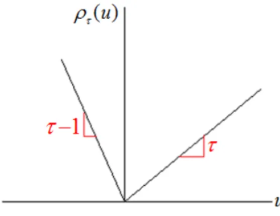
A more formal approach is to define the following loss function ( )u u ( I u( 0))



     (2.1)

which is depicted in Figure 2.1. Notice that although the loss function is continuous and linear, it is not differentiable at 0. For u0 the slope is  and for u0 the slope is  1. Now we aim to minimize

[ ( )] [( ) { ( 0)}] E _ Y E Y    I Y  ( 1) (y )dF u( ) (y )dF u( )          

_

 

_

 .

We can differentiate it with respect to  and solve

( ) (1 ) ( ) ( ) ( ) 0 U  dF y dF y F          







   .

This implies that the minimum is achieved when 1

( ). F  _   Given data { (Y i_i 1,..., )}n , define 1 ( ) ( ) ( ) / . n n n i i U  F   I Y  n     



  (2.2)

7 Hence the solution to U_n( )  or the minimum of 0





1 1 1 1 ( ) ( ) ( ) ( 0) n n n i i i i i R Y Y I Y n  n         



 



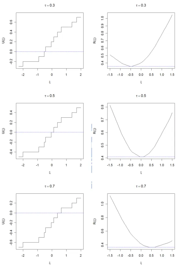
    (2.3) is attained at ˆ Q_Y( ) .

Now we plot U_n( ) and ( )R_n  for Yi ~iid N(0,1) (i1,...,10). These data

points are -2.002, -0.914, -0.526, -0.446, -0.052, 0.120, 0.386, 0.647, 1.379, 1.705. Note that 1(0.3)-0.524, 1(0.5)0 and 1(0.7)0.524. In Figure 2.2, we present two plots: (a)  versus ( )U_n  and (b)  versus R_n( ) based on

( )u u ( I u( 0))



     with  0.3, 0.5, 0.7. Our first purpose is to see the shapes of the two functions and whether the solution to U_n( )  or the minimum 0 of ( )R_n  are closed to 1(0.3), 1(0.5) and 1(0.7) respectively. In Figure 2.2, we see that is a monotone step function and can be well approximated by a convex function. These nice properties are useful for numerical computations and large-sample analysis.

2.2 Inference based on quantile regression analysis

In presence of covariates, the quantile regression model can be written as ( | ) ( ) T ( )

Y

Q  Z   Z   . (2.4)

Give data {( ,Y Z_{i i}) (i1,..., )}n , the objective function can be written as 1 1 ( ( ), ( )) ( ( ) ( )) n T n i i i R Y Z n            



 





1 1 ( ( ) ( )) ( ( ) ( ) 0) n T T i i i i i Y Z I Y Z n           



      . (2.5)

The major purpose is to minimize R . For illustration, we may first review the _n

problem based on minimizing the squared loss function such that

2 1 ( , ) ( ) n T n i i i R   Y  Z   



   .

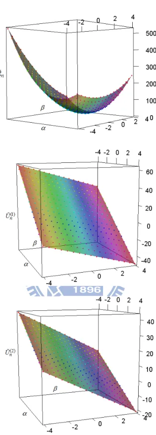
8 estimating function (1) ( 2) 1 1 ( , ) ( ) n n T n i i i i n U U Y Z Z U        _{ } _ _        



   . (2.6) Notice that ( ) ( , ) k n

U   (k 1, 2) are both smooth linear planes. In Figure 2.3, we plot ( , ,  R and _n) ( , ,  U_n( )k ) (k 1, 2) based on 10 simulated data points from a simple regression model.

Now return to the quantile estimation problem. Although R_n is not differentiable, we can still derive the directional derivative. Specifically the directional derivative of R in direction _n w with p

wR and w 1 can be obtained as follows:











0 1 0 1 0 1 ( ( ), ) ( ( ) ) ( ( ) ) ( ) ( ( ) 0) ( ) ( n n t n T i i i t n T T T T i i i i i i i t n T i i i i d R w R tw dt d Y Z tw dt d Y Z Z tw I Y Z Z tw dt Z w I Y Z                 _                    







          















1 ( ) 0) ( ) 1 ( ( ) 0) , T n T T i i i i Z w I Y Z        



        

where Z_i (1,Z_i)T and  ( )( ( ), ( ))    T. In general, we get the estimating function









(1) ( 2) 1 1 1 ( ( ), ( )) = ( ) ( ) 0 (1 ) n n T n i i i i n U U I Y Z Z n U               _ _{  }         



. (2.7)

This implies that  ( ) and   can be estimated by either minimizing ( ) R or n

solving 0U_n  .

9 ( | ) ( ) ( )

i

Y i i

Q  Z     Z (i1,...,10)

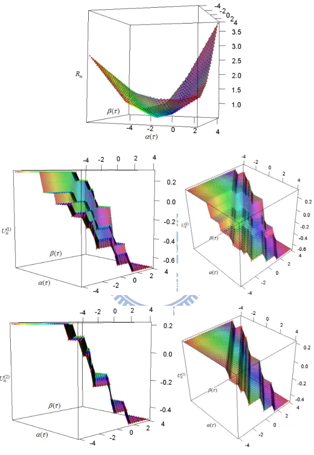
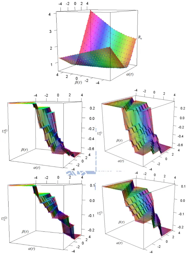
where  ( ) is the  -quantile from a standard normal distribution and  ( )3.5 . We will use these points to show several 3-D plots in Figure 2.4 and 2.5. Then we set

0.3

  and plot ( ( ), ( ),    R_n) and ( ( ), ( ),    U_n( )k ) where k 1, 2,  ( ) is

1

( )



 _{and there are two forms of} Z, namely Binomial(n, 1/2) and Uniform(0,1). Comparing Figures 2.4 and 2.5 with Figure 2.3, we see that the estimating

functions for the former may not take value at 0. As a result , the numerical algorithms to implement the estimation need special techniques.

2.3 Numerical algorithms

To simplify the notations, from now on we let Z and  ( ) include the intercept term. Numerical algorithms are needed to find the estimator of  ( ) which minimizes ( ( ))R_n   or solves U_n( ( ))   . Both problems are non-trial since the 0 functions are not differentiable so that the powerful Taylor-expansion technique cannot be directly applied.

2.3.1 Minimizing the objective function

Before introducing the algorithm, it is worthy to discuss the geometric structure behind the minimization problem. Consider the subspace spanned by

1

( ,..., )

T T

j  Zj Zjn

Z for j1,...,p and let YT ( ,...,Y₁ Yn)T denote the center. The

mechanism of the squared loss function behaves like a ball which inflates until the ball touches the surface of the above subspace. Now consider the problem of minimizing





1 1 1 1 ( ( )) ( ( )) ( ( )) ( ( ) 0) n n T T T n i i i i i i i i R Y Z Y Z I Y Z n  n             



 



    . The mechanism behaves like a polyhedral diamond, also centered at Y , expands until it touches the subspace.

10 Now we compare the solutions based on minimizing R_n( ) and R_n( ( ))  respectively. Since R_n( ) is differentiable, the solution is obtained by solving

( ) / 0

n

R  

   equivalent to Z YT( ZT)0. From a geometric viewpoint, it implies that the columns of Z are perpendicular to the error vector. Usually the estimator is obtained by solving the linear equations of  analytically. On the other hand, the directional derivatives of R_n( ( ))  is given by









1 ( ( ), ) ( ) 1 ( ( ) 0) . n T T n i i i i R   w Z w  I Y Z     



    

Geometrically moving away from   will increase ( ( ))ˆ( ) R_n   . A solution which minimizes R_n( ( ))  subject to R_n( ( ), )  w  will only occur at vertex 0 points. This implies that we only need to examine over all vertex points about which one satisfies the constraint. Analytically, the solution which minimizes R_n( ( ))  denoted as   must satisfy ˆ( ) R_n( ( ), ) ˆ w 0 for all wRp.

Using the terminology of linear programming, the candidate solutions are called as the “basic solutions”. A nice feature of these basic solutions is that they can be represented by a linear combination of p -component sub-matrix of Z and sub-vector of Y . Specifically let hH be the set with each element containing p

-numbers from {1, 2,..., }n and hence H consists of n p

   

  members. Denote

( ) :h pp

Z as the sub-matrix of Z with rows (Zi₁,...,Zip) for ih and ( ) :h p1

Y as the sub-vector of Y with elements Y_i for ih . The basic solution denoted as  _h( ) satisfies

 _h( ) Z( )h 1Y( )h . Hence we only need to check whether

11









1 ( ( ), ) ( ) 1 ( ( ) 0) 0 n T T n h i i i h i R   w Z w  I Y Z     



     

for all wRp. Recall that there are n

p

   

  candidates of h and how to examine the above inequality in all dimensions analytically is not straightforward.

The following equivalent expressions are useful for developing the numerical algorithm: _n( _h( ), ) ( ( _i 0)) _i T( ) i h R   v  I v v  h v    



    (2.8) where ( )vZ h wRp, T( ) *



_{i i}T _h( ), _iT ( ) 1



_iT ( ) 1 i h h _ Y Z Z h v Z h        



  Z Z and * _{1 2} 1 1 2 1 ( 0) if 0 ( , ) ( 0) if 0 I u u u u I u u           _{  }  .

It suffices to check whether R_n( _h( ), )v  for all 0 v e_k (k 1,..., )p which is equivalent to the following condition

( ) (1 )

p h p

  

 1    1 .

The above analysis simplifies the complicated minimization problem to the analytic objective of finding  _h( ) Z( )h 1Y( )h which satisfies 1_p ( )h  (1 )1 . _p

This is equivalent to 1 1 1 ( 1) sign( ( )) ( ) . 2 2 T p i i h i p i h Y Z Z h            _    _   



1 Z 1 (2.9) Thus we have 2 p inequalities in  of the form which can be viewed as

(  1) a_j b_j  (j1,..., )p

(2.10)

where (a b_j, _j) can be determined given the data and the basic solution. Notice that the above inequalities can be used to (a) find an appropriate  _h( ) from all the vertex points given the value of  or (b) given a vertex point, to find the corresponding value (or range) of  .

12 Now we briefly describe the algorithm. We can start from ₀ 1/ n which corresponds to the basic solution say

0 1 0 0 ( ) ( ) ( ) h h h   _{ Z}  Y by checking the 2 p

inequalities from all the n

p

   

  candidates of basic solutions. Then we find 1 which

corresponds to the basic solution

1 1 1 1 ( ) ( ) ( ) h h h   _{ Z} 

Y where h₀ and h₁ differ in one unit. It seems to us that the algorithm is to use the basic solutions

1

( ) ( ) ( )

h h h

  _{ Z} 

Y to find the corresponding value  satisfying 1 ( 1,..., ). (1 ) (1 ) j j j j a a j p b  b      

This algorithm only needs to perform a thorough search at the first time based on ₀. Then only a small variation in the basic solution is involved which changes the values of (a b which are used to find the next _j, _j) ₁. The procedure can go on until the targeted largest  is found.

2.3.2 Solving the estimating function by simulated annealing

Recall that









1 1 ( ( )) ( ) 0 (1 ) n T n i i i i U Z I Y Z n       



    .

Since ( ( ))U_n   is a step function which takes discrete values, it may happens that there exists no solution to U_n( ( ))   . Although the solution can be defined as the 0 value where the estimating function changes signs, an algorithm to find its location based on the data is still needed. One way of finding the solution is to transfer the root-solving problem into another minimization problem. Define ˆ( )  such that

ˆ ( ( ))

n

U   is minimized where U_n( ( ))  is the sum of the absolute values of the

p -components of U_n( ( ))  . Lin and Geyer (1992) suggested the simulated

annealing algorithm originally developed for a similar numerical problem in

13 under the context of quantile regression models.

Consider there are an old candidate *

( )

  and a new one **

( )

  . The old solution  *( ) will be replaced by  **( ) “for sure” if

** *

( ( )) ( ( )) 0

n n

D U    U    . This step is reasonable since obviously

**

( ( ))

n

U   is closer to zero. If D 0, the chance of  *( ) being replaced by

**

( )

  is exp(D c/ ). This means that the algorithm allows for an intermediate solution to move “farer away” from zero with the probability exp(D c/ ). We guess that the reason is to avoid the algorithm gets stuck in a local minimum point. Now the next question is how to come up with a new candidate  **( )? It is suggested that

**

( )

  has a (multivariate) normal random distribution with mean *

( )

  and a diagonal covariance matrix. This step implies that the position of the new  **( ) is related to the old one *

( )

  . Now we may ask what’s the principle for setting up the covariance matrix? It is suggested that, when the iterations continue, the variance of each component of **

( )

  and the value of c0 should decrease. The former implies that  **( ) gets closer to  *( ). The latter implies that if  **( ) does not reduce U_n( ( ))  , the chance that it replaces  *( ) gets smaller in the iterations.

The simulated annealing algorithm can be summarized below.

a. Give the initial values of (0)( ) , c(0) and 0  which is a diagonal matrix; (0) b. Generate a new  (1)( ) which follows N( (0)( ),(0));

c. If D U_n( (1)( ))  U_n( (0)( ))  , then replace 0 (0)( ) by  (1)( ) and otherwise replace (0)( ) by  (1)( ) with the probability exp



D c/ (0)



; d. Change the diagonal components of  and (0) c(0) to smaller numbers denoted

14 e. Repeat Steps (b) ~ (d) for k 1,...,m where m is a fixed value.

As for the initial values, Lin and Geyer (1992) made the suggestion: set (0)

( )

 

to zero; set the number of steps m1000p, where p is the dimension of  ( );  set “the cooling rate”  _for /2

0.0005

m

  ;  set initial variance as 0.1 and the cooling rate for the variances such that the diagonal components of  is about (m) 0.0005. The estimator is  ˆ( )( )m( ) which hopefully will get to the minimum of

( ( ))

n

U   .   

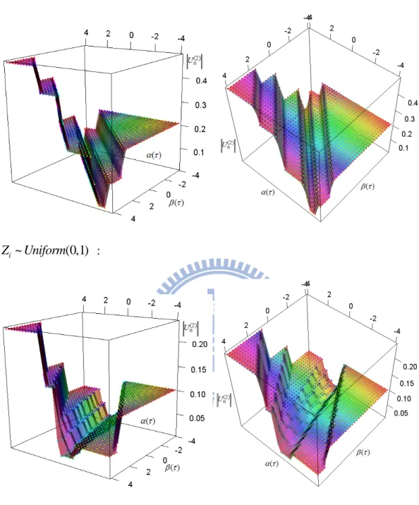
Now based on the simulated example, we present the second component of

( ( ))

n

U   and the movement of the algorithm. Figure 2.6 represents the cases of different types of Z .

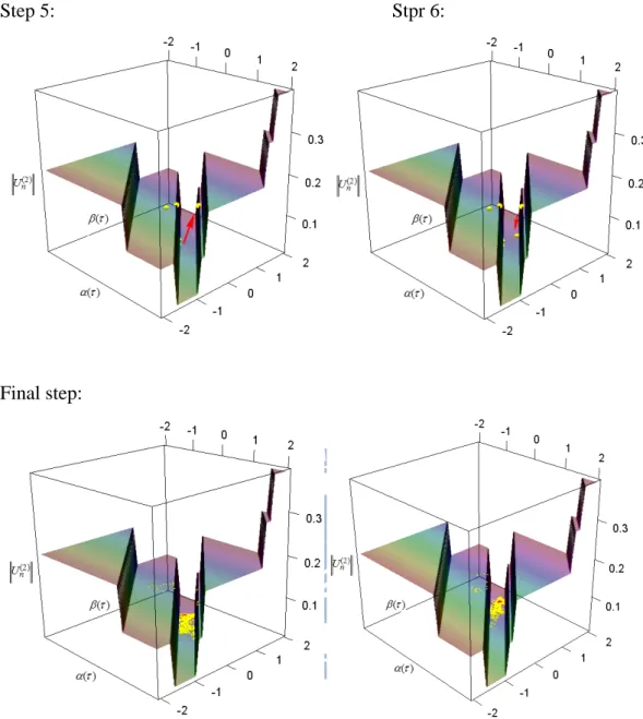
Now we present the intermediate steps of the algorithm in Figure 2.7. We see that the points still can jump up but finally the points come to the bottom and will not jump up anymore (convergence is reached). From our experience, we found that the choice of c(0) is influential. When this value is too large, the probability of jumping up becomes bigger while if it is small, there is higher chance that it remains unmoved. We set c(0)  U_n( (0)( )) 0.001 and also set the initial (0) 0.1 0

0 0.1

 

   

15

Chapter 3 Inference under Right Censoring

3.1 Data structure

Now we discuss quantile regression analysis based on survival data. Here the variable of interest is the time to the occurrence of an event of interest, denoted as T which is subject to censoring by C . Let Y log( )T and log( )C  C . The quantile

regression model can be written as

( | ) T ( )

Y

Q  Z Z   (3.1a)

or, based on the original failure time, such that

( | ) exp{ T ( )}.

T

Q  Z  Z   (3.1b)

Note that here Z and ( )  include the intercept term. Observed variables become ( , , )X  Z where X  Y C and  （I T  C). The main purpose is to estimate

( )

  based on data (X_i, ,_i Z_i) (i1,..., )n which is a random sample from ( , , )X  Z .

Several approaches to modifying the methods under censoring have been proposed. Here we summarize their main ideas and comment on their properties including drawbacks.

3.2 Modification based on the objective function

The paper by Powell (1986) was motivated by economic examples. The original construction is based on the situation that Y is subject to left censoring by 0, a _i

common phenomenon in economic applications. The idea can be easily modified for the situation that Y is subject to right censoring by a fixed value _i C . He used the _i

idea that minimizing a loss function based on Y_iZ_iT ( ) is equivalent to minimizing the same loss function based on {Y_iC_i} { Z_iT ( )C_i}. Accordingly the modified objective function can be written as

16 1 1 ( ( )) ( min{ , ( )}) n P T n i i i i R X C Z n        



 . (3.2)

The corresponding estimating function becomes





1 1 ( ( )) ( ( ) 0) ( ( ) ). n P T T n i i i i i i U Z I X Z I Z C n         



    

An obvious drawback of this approach is that C may be a random variable and also _i

subject to censoring. Furthermore R_nP( ( ))  in (3.2) is no longer a convex function and needs not be unimodal which creates numerical problems. To find the global minimum, excessive computation time is required.

To handle the censoring problem of C , Honoré, Khan and Powell (2002) _i

proposed to replace the loss function by its conditional expectation given (X_i, ,_i Z_i) in (3.2). That is, the objective function can be written as





1 1 ( ( )) min{ ( ), } ( , , ) n HP T n i i i i i i i R E X Z C X Z n           



_  _. Accordingly









[ _i min{ _iT ( ), _i} | _i, _i 0, _i] (1 _i) _i min{ _iT ( ), _i} E _ X  Z   C X   Z   _ X  Z   X and









 

[ min{ ( ), } | , 1, ] ( min{ ( ), }) ( ) T i i i i i i T i i i i i E X Z C X Z X Z c I X c dG c G X                 



where G t

 

Pr(Ct) can be estimated by the Kaplan-Meier estimator

1 1 ( , 1 ) ˆ ( ) {1 } ( ) n i i i n u t i i I X u G t I X u         







.

Notice that the above derivation requires that G t

 

does not depend on Z . The corresponding estimating function becomes

17 1 ( ( )) ˆ 1 (1 ) ( ( ) 0) ( ( )) ( ( ) 0) ˆ ( ) HP n T T n T i i i i i i i i i U I X Z G Z Z I X Z n G X                     _     _  



3.3 Modification based on the estimating function

Ying et al. (1995) proposed to directly modify the estimating function









1 1 ( ( )) ( ) 0 (1 ) n T n i i i i U Z I Y Z n       



    .

In presence of censoring, I Y( _i Z_iT ( )0) is not observable. Instead we observe

( _{i i}T ( ) 0)

I X Z    . Under the assumption that T_i and C are independent, it _i

follows that

E I X_



_iZ_iT ₀( )0



_ (1 ) (G Z_iT ₀( ))

where  ₀( ) is the true value of   and ( ) G t( )Pr(Ct) which can be estimated by the Kaplan-Meier estimator. Applying the technique of “inverse-probability-of-censoring-weighting”, they proposed the modified estimating function 1 1 ( ( ) 0) ( ( )) (1 ) ˆ ( ( )) T n YJW i i n i T i i I X Z U Z n G Z              _   _  



(3.2)

where I X( _i Z_iT ( )0) G Zˆ( _iT ( )) is zero if ˆ (G Z_iT ( )) is zero. The unconditional independence between T_i and C may be too restrictive and also _i

the weighting approach becomes invalid if the censoring support is shorter than the support of the failure variable.

3.4 A new approach based on counting process

The framework of counting process is useful for analyzing survival data in presence of censoring. Peng and Huang (2008) proposed a novel approach based on counting process to estimate the quantile regression parameter. We try to find a

18 motivation for their idea. Define F t_T( )Pr(T  and the corresponding cumulative t) hazard function can be written as _T( )t  log{1F t_T( )}. Consider the counting process N t( )I T( t). Under the standard setting, one often use the property that

0

( ) ( ) t ( ) _T( )

M t N t 



I T s d s (3.3) is a mean-zero martingale when _T(.) is the true function. One major advantage of the above decomposition is that N t and (( ) I T  can easily be modified under s) right censoring.

Notice that (3.3) holds when tQ_T( ) . That is,

( ) 0

( _T( )) ( _T( )) QT ( ) _T( )

M Q  N Q  



 I T s d s

which has a mean-zero property. The key result of Peng and Huang (2008) is the re-expression of the cumulative hazard function by substituting the range of integration from the scale of time to the scale of probability. Notice that

1 ( ) ( ) 1 0 0 0 ( ( )) QT ( ) FT ( ) ( ) T QT d T t d T t d T FT u        

_

 

_

 

_

 _ . Furthermore define 1 1 ( ) _{T T} ( ) log(1 _{T T} ( )) log(1 ) H u   _F u   F _F u   u . Thus 1 ( ) ( ) 0 0 0 ( ( )) QT ( ) FT ( ) ( ). T QT d T t d T t dH u       

_

 

_

 

_

In the paper, the original model assumption based on Y_i logT_i with

( | ) ( )

i

T

Y i i

Q  Z Z  

which is re-expressed based on T_i such that

( | ) exp{ ( )}

i

T

T i i

Q  Z  Z   for (0,1).

Another “trick” they used is to re-express (I X_i s) for sexp{Z_iT ₀( )} as

0

( _i exp{ _iT ( )})

19



exp{ 0( )}



₀



exp{ 0( )}



( ),

T T

i i i i

N Z   



I X  Z  u dH u (3.4) where  ₀( ) is the true value of  ( ) and ( )N t is sample analogs of _i N t for ( )

1,...,

i n. Note that (3.4) has a mean-zero property. Their proposed estimating function can be written as









1 2 0 1 ( ( )) exp{ ( )} exp{ ( )} ( ) n PH T T n i i i i i i U   n Z N Z   I X Z  u dH u     _   _  





. (3.5) To solve the equation U_nPH( ( ))  0 is not an easy task since to estimate

( )

  one needs to know the (estimated) value of ( )u for all u . Consider the set of grid points: S_L{0₀   ₁ ... _L _U 1} , where _U is a constant representing the upper bound of the identifiable region due to censoring. The authors

suggested a grid-based estimation procedure for  ₀( ) . Denote ( ) 



as an estimator of  ₀( ), which is a right-continuous piecewise-constant function that jumps only on the grid S_L{0₀   ₁ ... _L _U  Note that the attention of 1} this approach is (0,_U], not (0,1). It is suggested that the equation is solved successively for j1,...,L such that





1





1 2 1 1 0 exp{ ( )} exp{ ( )} ( ) ( ) 0, j n T T i i i j i i k k k i k n Z N Z   I X Z   H  H   _          _  _  _  _{  }





(3.6) where  ( )j 

is the solution to the equation. Notice that since the equation is not continuous, there may not exist an exact root. The algorithm of simulated annealing can be applied. A nice feature of the above estimating function is that it is a monotone function. This property is useful to develop a more efficient algorithm for numerical computation. Specifically, Peng and Huang (2008) found that solving (3.6) is equivalent to minimize the following objective function

20





* 1 1 1 * 1 1 0 ( ) log 2 exp{ ( )} ( ) ( ) n n T T j i i i i l l i l j n T T r r r k k k r k l h X h Z R h Z R h Z I X Z H H           _          _{ }    _{ }  _  _    









where R is a very large number and * j1,..,m. Peng and Huang (2008) mentioned that one advantage of the latter formulation is that the Barrodale-Roberts algorithm (Barrodale and Roberts 1974) can be directly applied. We do not investigate further in this direction.

3.5 A new approach based on self-consistency algorithm

Portnoy (2003) proposed a method which utilizes the idea of self-consistency based on the Kaplan-Meier estimator. Specifically the Kaplan-Meier based on data {(X_i, ) (_i i1,..., )}n can be written as 1 1 ( , 1) ˆ ( ) {1 } ( ) n i i i Y n u y i i I X u S y I X u         







.

Alternatively it also satisfies:

1 ( ) 1 ( ) ( , 0) ( ) ( ) n Y Y i i i i Y i S y S y I X y I X y n   S X    _     _  



.

That is, the “weight” contributed to estimate S_Y( )y for an observation _{X with i}

i X  and y _i 0 _is ( ) ( ) Y Y i S y

S X . Now we return to the quantile problem. Setting

( ) 1

Y

S y   and ( ) 1 S_Y X_i   where _i  _i  , we have

1 1 1 1 ( ( ), 0) ( ( )) 1 n i Y i i Y i i I X Q I X Q n             _     _   



. This is equivalent to 1 1 ( ( ), 1) ( ( ), 0) 1 n i i Y i i Y i i i I X Q I X Q n              _      _   



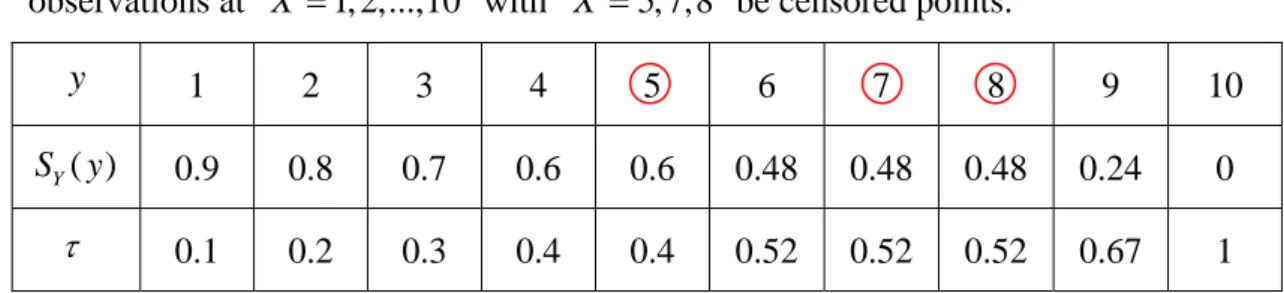
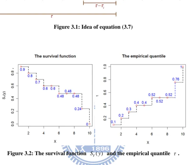
. (3.7)

21 Figure 3.1 shows the idea of (3.7). For example, there is a single sample with 10 observations at X 1, 2,...,10 with X 5, 7,8 be censored points.

y _{1 2 3 4 5 6 7 8 9 10}

( )

Y

S y 0.9 0.8 0.7 0.6 0.6 0.48 0.48 0.48 0.24 0

 _{0.1 0.2 0.3 0.4 0.4 0.52 0.52 0.52 0.67 1}

In Figure 3.2, we can see that S_Y( )y and the empirical quantile  are both step

functions but the former is decreasing, while the latter is increasing. Notice that the value of empirical quantile  is equivalent to 1 minus the corresponding value of

( )

Y

S y . Now we select Q_Y(0.52) . It is clear that 6

1 0.52 1 0.52 ( 6, 1) ( 6, 0) 1 n i i i i i i i I X I X n          _      _   



, which results in 1 0.52 0.4 0.52 (5 ) 10 1 0.4     .

This implies that a censored observation with _i 0 _{will contribute the weight} ( ) 1 i i i w      

 . Note that the proposed algorithm is based on minimizing





1 ( ) ( ) n T i i i i w  _ X Z    



where 0, ( ) , and 0 1 1, and 1 i i i i i i i i w                _  _{ }     _{ }  .

The idea proposed by Portnoy (2003) is novel, but it is hard to understand the details. Later work by Neocleous, Branden and Portnoy (2006) and Portnoy and Lin (2010) provide more explanations on the self-consistency algorithm.

22

Chapter 4 Conclusion

In this thesis, we review literature on quantile regression models. Comparing with other regression models, the quantile regression model is more flexible without imposing strong assumption on the error distribution and can well explain the heterogeneity data. Unlike the squared loss function in the least squared regression method, the loss function for estimating the quantile is not differentiable. Accordingly many nice analytic approaches such as the Newton-Raphson method are no longer applicable. Nevertheless, without censoring, some nice analytic properties such as monotonicity and convexity for the estimating and objective functions still exist. They are also helpful for developing numerical algorithms to implement the estimation. When censoring is present, how to modify the estimation procedures and how the modifications affect the analytical properties are the main issues. The thesis is just an initial review for these useful but complicated methods. Thorough investigation to understand these methods better deserve future study.

23

Figure 1.1: Definition of  th quantile.

Figure 1.2: Quantiles for two samples.

24

25

Figure 2.3: Objective and estimating functions based on LSE with

~ (1 2)

i

26

Figure 2.4: Plots of ( ( ), ( ),    R_n) and ( ( ), ( ),    U_n( )k ) (k 1, 2) based on

27

Figure 2.5: Plots of ( ( ), ( ),    R_n) and ( ( ), ( ),    U_n( )k ) (k 1, 2) based on

28 ~ (1 2) i Z Bernoulli : ~ (0,1) i Z Uniform :

Figure 2.6: Plots of U_n(2)( ( ))  based on Z_i ~Bernoulli(1 2) and

~ (0,1)

i

29 Step 1: initial point Step 2:

30

Step 5: Stpr 6:

Final step:

31

Figure 3.1: Idea of equation (3.7)

32

References:

[1] Barrodale, I., and Roberts, F. D. K. (1974), “Solution of an Overdetermined System of Equations in the _{ Norm,” Communications of the ACM, 17, 1} 319-320.

[2] Honoré, B., Khan, S., and Powell J. L. (2002), “Quantile Regression Under Random Censoring,” Journal of Econometrics, 109, 67-105.

[3] Lin, D.Y., and Geyer, C. J. (1992), “Computational Methods for Semiparametric Linear Regression with Censored Data,” Journal of Computational and

graphical Statistics, 1, 77-90.

[4] Necleous, T., Branden, K. V., and Portnoy, S. (2006), “Correction to Censored Regression Quantiles by S. Portnoy, 98 (2003), 1001-1012,” Journal of the

American Statistical Association, 101, 869-861.

[5] Peng, L., and Huang, Y. (2008), “Survival Analysis with Quantile Regression Models,” Journal of the American Statistical Association, 103, 637-649. [6] Portnoy, S. (2003), “Censored Regression Quantiles,” Journal of the American

Statistical Association, 98, 1001-1012; Corr, 101, 860-861.

[7] Portnoy, S., and Lin, G. (2010), “Asymptotics for censored regression quantiles,”

Journal of Nonparametric Statistics, 22, 115-130.

[8] Powell, J. L. (1986), “Censored Regression Quantiles,” Journal of Econometrics, 32, 143-155.

[9] Ying, Z., Jung, S. H., and Wei, L. J. (1995), “Survival Analysis with Median Regression Models,” Journal of the American Statistical Association, 90, 178-184.

[10] Koenker, R., and Geling O. (2001), “Reappraising Medfly Longevity: A Quantile Regression Survival Analysis,” Journal of the American Statistiical Association, 96, 458-468.

33 [11] Koenker, R., and V. D’Orey (1987), “Computing Regression Quantiles,” Journal

of the Royal Statistical Society, 36, 383-393.

[12] Koenker, R. (2005), Quantile Regression, Cambridge: Cambridge University Press.

34

Appendix

A.1 Data generation from a quantile regression model

Usually to generate Y which has the distributional function F_Y(.), we can generate U ~U(0,1) and set Y F_Y1( )U . Consider the objective that, given Z , we _i

want to generate Y which follows _i

Pr(Y_i Z_iT ( ))  (i1,...,n). Generate ~ (0,1)

iid i

U U . Setting Y_i Z_iT(U_i) and suppose that ZT( )t is a monotone increasing function of t , it follows that

Pr(Y_iZ_iT ( ) |Z_i)Pr(Z_iT(U_i)Z_iT ( ))Pr(U_i ) . 

The next question is how to set the distribution of Y as a target one. Consider a _i

simple two-sample case with Z_i ~Bernoulli p( ). Notice that

0

Pr(Y_i  ( ) |Z_i 0)F ( ( ))  

which means that the intercept  ( )F₀1( ) is the quantile of the baseline group. Suppose we let Y Z_i| _i 0 be the standard normal distribution, we should set

1

( ) ( )

  _{ } 

which is the quantile of N(0,1). It follows that Y Z_i| _i 1 ~N( ( ),1)  . The algorithm is summarized below:

Step1: Generate Z_i ~Bernoulli p( ) and U_i ~Uniform(0,1).

Step2: Let (U_i) 1(U_i) and (U_i)c U_{0 i} where  is the cumulative distribution function for N(0,1) and c is a constant. ₀

Step3: Set Y_i (U_i)Z_i(U_i).

35 Now let n500, p1 2 and c₀ 1.5. Then we generate data from a

quantile regression model by the following codes of R: n=500; b=1.5; Z=sample(c(0,1), size=n, replace=TRUE); u=runif(n,0,1); btau=b*u; Y=array(0,n);

Y=qnorm(u)+Z*btau windows(); plot(Z, Y);

Figure A.1 shows that the two groups of generated data (Z Y_i, )_i (i1,...,n) with the control group (Z_i 0) and the treatment group (Z_i 1). To check the normality for the control group, we can examine Figure A.2 which provides a histogram plot and the Q-Q plot which show that Y Z_i| _i 0 is exactly generated from a standard normal distribution. Notice that

1

Pr(Yi  ( ) ( ) |Zi  1) F( ( )   ( ))

which means that the slope 1 1

1 0

( ) F ( ) F ( )

 _{ }   _  

is the quantile treatment effect, illustrated in Figure A.3. To check the accuracy of generated data, we plot the empirical quantile functions and the corresponding theory functions of F and ₀ F ₁

in Figure A.4. Note that the empirical functions of F and ₀ F are ₁

1 0 1 ( , 0) ˆ ( ) ( 0) n i i i n i i I Y y Z F y I Z      





  and 1 1 1 ( , 1) ˆ ( ) ( 1) n i i i n i i I Y y Z F y I Z      





  .

From Figure A.4, we see that both empirical quantile functions match the corresponding theory functions very well. That is, our data generation from a quantile regression model is correct.

Because the objective function is not differentiable, to evaluate the estimation procedures, we make 2-D plots of



 ( ),R_n( ( )) 



and



 ( ),R_n( ( )) 



for given

0.3, 0.5, 0.7

36





1 1 ( ( ), ( )) ( ( ) ( )) ( ( ) ( )) ( ( ) ( ) 0) . n n i i i n i i i i i R Y Z Y Z I Y Z                               





      

Note that, to get the plots of



 ( ),R_n( ( )) 



, we set  ( )c₀ which is known, whereas  ( ) 1( ) as known for getting the plots of



 ( ),R_n( ( )) 



. In Figure A.5, we see that there is a minimum for the parabolic curve in each panel and these are the estimators of ( )  and ( )  which are marked by blue points. It

shows that the estimators of  ( ) and ( )  are close to the true values  0( ) and

0( )

  which are marked red dash lines. Figure A.5 is made by the following codes of

R:

alpha=seq(-5, 5, by=0.1); beta=seq(-5, 8, by=0.1); for(k in 2:4) {

tau=0.1*(2*k-1); windows(); par(mfrow=c(1,2)); Ra=array(0, length(alpha)); Rb=array(0, length(beta))

amax=-2^31; amin=2^31; bmax=amax; bmin=amin; for(i in 1:length(alpha)) {

for(j in 1:n) {

if(Y[j]<alpha[i]+Z[j]*b*tau)

Ra[i]=Ra[i]+(Y[j]-alpha[i]-Z[j]*b*tau)*(tau-1) else Ra[i]=Ra[i]+(Y[j]-alpha[i]-Z[j]*b*tau)*tau } if(Ra[i]> amax) amax=Ra[i]

if(Ra[i]< amin) {

amin=Ra[i]; ax=alpha[i] } }

plot(alpha, Ra, type='l', xlab=expression(alpha(tau)),

ylab=expression(paste('R(',alpha(tau),')'))) title(main=substitute(list(tau)==list(a), list(a=tau)))

abline(v=qnorm(tau), col='red', lty=2)

37 list(a=round(qnorm(tau),3))), col='red')

points(ax, amin, col='blue')

text(ax, amin+350, substitute(list(hat(alpha)(tau))==list(a),

list(a=round(ax,3))), col='blue') for(i in 1:length(beta)) { for(j in 1:n) { if(Y[j]<qnorm(tau)+Z[j]*beta[i]) Rb[i]=Rb[i]+(Y[j]-qnorm(tau)-Z[j]*beta[i])*(tau-1) else Rb[i]=Rb[i]+(Y[j]-qnorm(tau)-Z[j]*beta[i])*tau }

if(Rb[i]> bmax) bmax=Rb[i] if(Rb[i]< bmin) {

bmin=Rb[i]; bx=beta[i]; } }

plot(beta, Rb, type='l', xlab=expression(beta(tau)),

ylab=expression(paste('R(',beta(tau),')'))) title(main=substitute(list(tau)==list(a), list(a=tau)))

abline(v=b*tau, col='red', lty=2)

text(b*tau+0.2, bmax-100, substitute(list(beta[0](tau))==list(a),

list(a=round(b*tau,3))),col='red') points(bx, bmin,col='blue')

text(bx, bmin+250, substitute(list(hat(beta)(tau))==list(a),

list(a=round(bx,3))), col='blue') } Now we do the data generation from a quantile regression model 100 times. The mean, variance and biased for the estimators of  ( ) and ( )  are presented in the following:

Estimator of  ( ) Estimator of  ( )

Mean Variance Bias Mean Variance Bias

0.1   -1.269 0.0076 0.0125 0.164 0.019 0.014 0.3   -0.524 0.0052 4 4 10  0.46 0.01777 0.01 0.5   16 2 10  0.0056 2 10 16 0.747 0.01625 -0.003 0.7   0.511 0.0056 -0.0134 1.038 0.01874 -0.012 0.9   1.273 0.0066 -0.0085 1.331 0.01953 -0.019

38 From the table, we see that the values of bias are very small for all  .That is, the average values of the estimators are closed to the true value  ₀( ) and  ₀( ).

A.2 How to generate the 3-D plots

To show how to generate the 3-D plots in R, we take Figure 2.4, Figure 2.5 and Figure 2.6 as examples. Note that the functions for 3-D plots are in package

scatterplot3d and rgl for R. If you are the first time to make a 3-D plot, you must

install them and load them into R. The code of 3-D plot for R is as follow: ###Loading these packages

library(scatterplot3d) ; library(rgl);

### Data generate n=10; b=3.5; tau=0.3;

Z=sample(c(0,1),size=n,replace=TRUE); u=runif(n,0,1); btau=b*u; Y=array(0,n); Y=qnorm(u)+Z*btau;

### Range of alpha and beta

alpha=seq(-4, 4, by=0.5); beta=seq(-4, 4, by=0.5)

a=array(rep(c(alpha), each=length(beta)), length(alpha)*length(beta)) b=array(rep(c(beta), times=length(alpha)), length(alpha)*length(beta))

### 3-D plot for R(.)

R=array(0, length(alpha)*length(beta)) ; NR=array(0, length(alpha)*length(beta)); for(k in 1: length(alpha)) { for(s in 1: length(beta)) { for(j in 1: n) { if(Y[j]< alpha[k]+beta[s]*Z[j]) R[s+(k-1)*length(beta)]= R[s+(k-1)*length(beta)]+(Y[j]-alpha[k]-beta[s]*Z[j])*(tau-1)/n else R[s+(k-1)*length(beta)]= R[s+(k-1)*length(beta)]+(Y[j]-alpha[k]-beta[s]*Z[j])*tau/n }

39 NR[k+(s-1)*length(alpha)]=R[s+(k-1)*length(beta)] } }

col=rainbow(length(alpha)*length(beta)) open3d()

plot3d(a, b, R, pch=176, col=col, type='p', xlab="alpha", ylab="beta",

zlab=" R(tau)", smooth=FALSE) surface3d(alpha, beta, NR, col=col, alpha=0.65)

### 3-D plot for U1(.)

U1=array(0, length(alpha)*length(beta)); NU1=array(0, length(alpha)*length(beta)) for(k in 1: length(alpha)) { for(s in 1: length(beta)) { for(j in 1: n) { if(Y[j]< alpha[k]+beta[s]*Z[j]) U1[s+(k-1)*length(beta)]=U1[s+(k-1)*length(beta)]+(tau-1)/n else U1[s+(k-1)*length(beta)]=U1[s+(k-1)*length(beta)]+tau/n } NU1[k+(s-1)*length(alpha)]=U1[s+(k-1)*length(beta)] }} col=rainbow(length(alpha)*length(beta)) open3d()

plot3d(a, b, U1, pch=176, col=col, type= 'p',xlab="alpha", ylab="beta",

zlab=" U1(tau)") surface3d(alpha, beta, NU1, col=col, alpha=0.65)

### 3-D plot for U2(.)

U2=array(0, length(alpha)*length(beta)); NU2=array(0, length(alpha)*length(beta)) for(k in 1: length(alpha)) { for(s in 1: length(beta)) { for(j in 1: n) { if(Y[j]< alpha[k]+beta[s]*Z[j]) U2[s+(k-1)*length(beta)]=U2[s+(k-1)*length(beta)]+Z[j]*(tau-1)/n else U2[s+(k-1)*length(beta)]=U2[s+(k-1)*length(beta)]+Z[j]*tau/n } NU2[k+(s-1)*length(alpha)]=U2[s+(k-1)*length(beta)] } }

40 col=rainbow(length(alpha)*length(beta))

open3d()

plot3d(a, b, U2, pch=176, col=col, type= 'p',xlab="alpha", ylab="beta",

zlab=" U2(tau)") surface3d(alpha, beta, NU2, col=col, alpha=0.65)

### 3-D plot for ||U(.)||

U=array(0, length(alpha)*length(beta)); NU=array(0, length(alpha)*length(beta)) for(k in 1: length(alpha)) { for(s in 1: length(beta)) { for(j in 1: n) { if(Y[j]< alpha[k]+beta[s]*Z[j]) U[s+(k-1)*length(beta)]=U[s+(k-1)*length(beta)]+Z[j]*(tau-1)/n else U[s+(k-1)*length(beta)]=U[s+(k-1)*length(beta)]+Z[j]*tau/n } U[s+(k-1)*length(beta)]=abs(U[s+(k-1)*length(beta)]) NU[k+(s-1)*length(alpha)]=U[s+(k-1)*length(beta)] } } col=rainbow(length(alpha)*length(beta)) open3d()

plot3d(a, b, U, col=col, type= 'p',xlab="alpha", ylab="beta", zlab=" U(tau)") surface3d(alpha, beta, NU, col=col, alpha=0.65)

41

Figure A.1: Scatterplot of generated data from a quantile regression model.

Figure A.2: Histogram plot and Q-Q plot of Y Z_i | _i 0.

42

Figure A.4: Plots of the empirical quantile functions and the corresponding theory functions of F and ₀ F . ₁